A Hybrid Genetic Programming and Boosting Technique
for Learning Kernel Functions from Training Data
Marta Gîrdea
“Alexandru Ioan Cuza” University of Ia¸si
Faculty of Computer Science
16 General Berthelot, Ia¸si, România
[email protected]
Liviu Ciortuz
∗“Alexandru Ioan Cuza” University of Ia¸si
Faculty of Computer Science
16 General Berthelot, Ia¸si, România
[email protected]
Abstract
This paper proposes a technique for learning kernel functions that can be used in non-linear SVM classifica-tion. The technique uses genetic programming to evolve kernel functions as additive or multiplicative combinations of linear, polynomial and RBF kernels, while a procedure inspired from InfoBoost helps the evolved kernels concen-trate on the most difficult objects to classify. The kernels obtained at each boosting round participate in the training of non-linear SVMs which are combined, along with their confidence coefficients, into a final classifier. We compared on several data sets the performance of the kernels obtained in this manner with the performance of classic RBF kernels and of kernels evolved using a pure GP method, and we concluded that the boosted GP kernels are generally better.
1. Introduction
In classification and clustering problems, the success of the classifier is determined, among other factors, by the quality of the similarity measure. Placing objects in classes with respect to their features requires a comparison between objects and a partition of the object space according to the results of this comparison. Classification problems may be-come more difficult if the similarity measure between ob-jects to be classified is not obvious. Therefore, it is often useful to attempt to learn the similarity function, rather than use a default one that may not be appropriate in some cases. This paper concentrates mostly on learning kernel func-tions that can be used by SVM classifiers [7, 26], in which direction few attempts have been made. Existing
ap-∗This paper was published inProceedings of SYNASC 2007, The 9th International Symposium on Symbolic and Numeric Algorithms for Scientific Computing, Timi¸soara, Romania, IEEE Conference Publishing, 2007.
proaches to learning kernel functions use machine learning instruments such as genetic algorithms or genetic program-ming [8, 9, 25] or boosting [14] in order to design kernel functions that best explain the available data.
We propose a method that uses genetic program-ming [16] to evolve a kernel function as a combination of linear, polynomial and RBF kernels. A boosting procedure, inspired from InfoBoost, is used to help the evolved kernels concentrate on the most difficult objects to classify, and to obtain a final model with a low generalization error on un-seen data.
The organization of this paper is as follows: section 2 de-scribes the problem that the paper aims to solve: learning, from training data, kernel functions for SVMs; section 3 is a brief overview of other approaches having the same pur-pose; section 4 presents the proposed approach, which in-volves genetic programming and InfoBoost; some results are presentend in section 5 and discussed in section 6; the paper concludes with section 7.
2. Context and problem description
2.1. Support Vector Machines
Support Vector Machines (SVM) [4, 23, 26, 27] are robust instruments for classification. Given the set S ({(xi, yi)}, xi ∈ Rd, yi ∈ {−1,+1}), each element
be-longing to the positive (labeled +1) or to the negative (la-beled -1) class, a separating hyperplane must be found for the two classes, maximizing the margin (the distance be-tween the hyperplane and each class). The support vectors are the data points on the boundary of each class, the clos-est points to the separating hyperplane. The hyperplane can be computed as a combination of these vectors, and they are usually significantly less numerous than the entire set of available data points.
2.2. Kernel functions
In real-life problems, we generally deal with classes that are not linearly separable in the given feature space. Non-linear SVMs are based on the idea that two classes which are not linearly separable in a spaceX ⊂Rnmay be
line-arly separable in a higher dimensional space,Rm. A
func-tion φ : X → Rm can be used to map instances in the
higher dimensional feature space. Considering that, when the separation hyperplane is computed, the instance vectors only appear in dot products. The “kernel trick” [1] is used to implicitly map input vectors to a higher dimensional space where an optimal separating hyperplane is constructed.
By definition, a kernel is a functionKsuch that, for all
x,z∈X,
K(x,z) =φ(x)·φ(z)
where φ is a mapping fromXinto an inner product fea-ture space F. According to Mercer’s theorem [19], any continuous, symmetric, positive semi-definite kernel func-tionK(x, y)can be expressed as a dot product in a high-dimensional space. Based on this statement, several func-tions can be proved to be (Mercer) kernels and are com-monly used in practice:
• Linear:K(x,x′) = (γx·x′+c)
• Polynomial:K(x,x′) = (γx·x′+c)q, forγ,candq >0 • Radial Basis Function: K(x,x′) = exp(−γkx−x′k2),
forγ >0
• Sigmoid: K(x,x′) = tanh(κx·x′+c), for some (not
every)κ >0andc <0
Based on the consequences of the same theorem, in order to verify that a new symmetric functionK :X×X →R is a kernel it suffices to check if it satisfies the requirement that the matrix defined by restricting the function to any fi-nite set of points inX is positive semi-definite. This crite-rion can be applied to confirm that a number of new, more complicated kernels can be created from other simpler ones. Thus, ifK1andK2are kernels overX×X, withX ⊆Rn,
x,z∈X,a∈R+, then the following are also kernels: K(x, z) =K1(x, z) +K2(x, z) (1)
K(x, z) =aK1(x, z) (2)
K(x, z) =K1(x, z)K2(x, z) (3)
2.3. Choosing a kernel
Choosing the right kernel for a specific classification problem can be a difficult task. There is no universal kernel that can be used in any classification. Moreover, for some problems, where the classes are not just linearly unsepara-ble, but also non-convex, with many border irregularities,
the choice of the kernel function becomes a delicate issue, since simple kernels, as well as kernels build “by hand”, based on human observations and intuition, may fail.
Naturally, in such cases, an automated search through the space of possible kernel functions should give a better an-swer to the optimal kernel problem. The main objective of this paper is to study methods of learning similarities (in this case, kernel functions that express such similarities) from the given data. Practically, we need a tool that can automat-ically find the best kernel function for the given data set.
3. Related work
There are several other approaches for learning kernels functions, the most notable of them involving boosting tech-niques and genetic programming.
KernelBoost [14] is an algorithm for learning kernel functions from labeled and unlabeled training data. It builds a strong kernel using boosting on a weak Gaussian Mix-ture Model (GMM) learner, constrained Expectation Max-imization [24]. The boosting process is combined with a dissolving mechanism, which breaks difficult, non-convex classes into subclasses that are more likely to be modeled by a Gaussian Mixture Model.
The paper [25] proposes an evolutionary strategy for multi-scale radial basis function kernels. In order to ob-tain a flexible kernel function, a family of radial basis func-tion (RBF) kernels is proposed. Multi-scale RBF kernels are combined by including weights. Then, the evolutionary strategies are used to adjust these weights and the widths of the RBF kernels.
Two more recent papers [8, 9] present a model for evolv-ing multiple kernel functions for Support Vector Ma-chines (SVM), which combines Genetic Programming and an SVM tool. The GP chromosome is a tree encoding the mathematical expression of the kernel function used by an SVM. The quality of a chromosome is the accuracy rate – i.e. the number of correctly classified items over the total number of items – which is obtained from an SVM classifi-cation that uses the kernel encoded by the given individual. The results obtained with these methods are comparable with, or better than those achieved using simple kernels. This encourages further research in kernel learning.
4. InfoBoosted GP Kernels
As explained in section 2, kernels can be built from other kernels as linear combinations or products. Using genetic programming [16] and some training data manage-ment strategies inspired by boosting [3, 13, 22], a composite kernel is evolved from the available data, based on simple li-near, polynomial and RBF kernels, agregated in linear com-binations or multiplications. The evolution process searches
for the appropriate structure in which the simple kernels are combined, as well as for the best values for the internal pa-rameters.
The learning process can be summarized as follows:
• each individual is a kernel, obtained as a combination of some basic kernels;
• an evolutionary process builds new kernels using genetic operators and encourages the propagation of the best fea-tures among the generations;
• training instances are sampled according to a distribution that emphasizes the most difficult instances at the moment; a sampling is used for several generations (a boosting round) as the environment that must be learned;
• the evaluation of a kernel consists of obtaining a classifi-cation over the sample using that kernel, and computing a “confidence” value for the individual as the correctness of the classification;
• the best individuals from each round are kept (offline) if they perform better than an established confidence threshold θ;
• update the distribution over the training data according to how the instances are classified using the best kernel of the round.
Several papers that propose a combination of boost-ing and genetic programmboost-ing already exist, most of them choosing AdaBoost as the learning meta-algorithm: [15, 17, 20]. Our work explores the possibility of using ideas from InfoBoost [3], with the purpose of getting a better evalua-tion of the weak learner’s outcome.
4.1. Genetic Programming elements
Genetic Programming [16] uses principles of darwinian evolution, such as genetic recombinations and survival of the fittest, in order to automatically discover computer pro-grams that perform a user-defined task. Like other evolu-tionary techniques, this method uses a population of indi-viduals (also called chromosomes), each individual repre-senting a computer program. Several transformations are applied to these chromosomes for obtaining a new popula-tion: crossover, mutation, reproduction, gene duplication, gene deletion.
Candidate kernel representation
The individual structures that undergo adaptation in genetic programming are computer programs, traditionally repre-sented in memory as tree structures. The size, the shape and the contents of these computer programs can dynamically change during the process. This aspect is particularly suited to the goal of the kernel function search process. We look
for a kernel function, not knowing in advance the shape or the complexity of this function. Not only parameters need to be found, but also the structure and componency of the function itself.
The set of possible structures in genetic programming is the set of all possible compositions of functions that can be composed recursively from a set of functionsF ={fi}and
a set of terminalsT ={ti}. The choice of theF andTsets
strongly depends on the problem that needs to be solved. In the case of kernel function search, the candidate solutions will be mathematical expressions of the kernels.
As explained in section 2, there are several operations that can help building new kernel functions from other ker-nel functions. We will further make use of the three rules, (1), (2) and (3), presented in that section. Consequently, the function set will contain the two arithmetic operations + and *, each with 2 arguments.
The terminal set will contain the nodes that represent some popular kernels used in practice:LK (linear kernel), P K(polynomial kernel) andRK(RBF kernel), along with randomly generated scalars. LK has 2 scalar parameters, P K has 3, andRK has one, necessarily positive, as pre-sented above. The scalars are Ephemeral Random Con-stants (ERC), as defined in [16], generated according to an exponential distribution in the range[e−10, e10), except
q, which is an integer in the range[1..100]. Genetic Operations
New candidate solutions from the search space are gen-erated in genetic programming (like in all evolutionary methods) by means of genetic operators. For each operator, some validity constraints need to be taken into considera-tion, in order to obtain correct expressions for the kernels.
The crossover operation for genetic programming pro-duces two new offsprings that are built of parts taken from each of the two parents. It consists of independently se-lecting a random point in each parent as the cut point for crossover, and switching between parents the rooted sub-trees that lie below the cut points.
Another genetic operator, called internal crossover, acts on a single individual, by randomly choosing two cut points and swapping the respective subtrees within the individual’s structure.
The mutation operation, which induces random changes in the individuals, ensuring diversity, is present in our method in three variants:
• a classic mutation operator on tree structures, that ran-domly chooses a node in the tree and replaces the whole rooted subtree that starts in the chosen node with a ran-domly generated subtree.
• a one node mutation operator, that randomly chooses a node in the tree and replaces it with another node, leaving
the rest of the subtree unchanged.
• a random number mutation, that only operates on the val-ues of the scalars in the expression tree.
Evaluation
The fitness function of an individual is a measure of the quality of that individual. The higher the fitness, the better adapted the chromosome, and, consequently, in this context, the better the kernel function it represents.
The fitness of a kernel function is here given by the ac-curacy of the classification performed by a non-linear sup-port vector machine that uses that kernel for the implicit mapping of the instances in the dataset. More precisely, an SVM is trained and tested on the given data set. The 4-fold cross-validation result of the classification, expressed as the number of correctly classified instances, is the fitness of the evaluated individual.
A very important detail of the evaluation process is the componency of the data set each individual is tested against. This is one of the aspects where boosting ideas are involved. At each round (group of generations), the individuals are evaluated on a different distribution over the data set, which will further result into the more probable survival of the ker-nels that were able to ensure the right classification of the instances that are usually misclassified.
The next section will give a brief overview of the boost-ing methods and provide technical details about the actual computation of this distribution.
4.2.
Boostingelements
Boosting – An overview
Practice shows that, for classification problems, finding a single strong rule that is valid for all (or at least almost all) data is considerably more difficult than finding several weak rules (rules of thumb), with moderate accuracy, that only apply in some cases. Moreover, the set of rules of thumb found with a simple method can be combined into a com-plex, strong rule, of high overall accuracy. This idea led to the boosting method and its variations.
Boosting [12, 22] is a machine learning meta-algorithm for supervised learning, mostly used in classification. It is based on weak learners – classifiers with an accuracy some-what better then random – and by combining their results, it obtains an accurate classifier. The term to boost suggests the purpose of this method: to grow, to enhance the accuracy of a learning algorithm.
The weak learner is trained at each boosting round on a different set of data, or on a different distribution, in order to obtain different classifiers that can separate the data in some cases. In the end, the obtained weak rules are combined into a single strong rule.
Within this general structure, some particular aspects must be specified: the choice of the distribution over the training data at each round, and the method for combining the weak rules into a strong rule.
InfoBoost
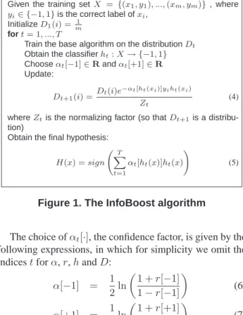
InfoBoost [3] was proposed as a modification of AdaBoost [13] on the computation of the confidence in the weak clas-sifier at each boosting round. AdaBoost (adaptive boosting) proposed that the distribution on each boosting round can be obtained by associating higher probabilities to the training instances that were misclassified, thus forcing the learner to concentrate on the difficult examples, while the strong rule can be the weighted vote combination of the weak rules, with weights – confidence coefficients – depending on the training error of the weak classifier. In [3] Aslam suggested that the qualitative and quantitative performance of a predic-tor is not entirely captured by error. Two weak hypotheses with the same error on the current distribution can actually have divergent behaviors, such as a lower false negative rate at the expense of a high positive rate and vice versa. Ex-ploiting more of the information that can be obtained about the weak learner’s performance is the purpose of InfoBoost (see figure 1), which proposes different confidence values for the positive and for the negative answer given by a weak hypothesis respectively.
Given the training setX = {(x1, y1), ...,(xm, ym)}, where
yi∈ {−1,1}is the correct label ofxi, InitializeD1(i) = m1
fort= 1, ..., T
Train the base algorithm on the distributionDt Obtain the classifierht:X→ {−1,1} Chooseαt[−1]∈Randαt[+1]∈R Update: Dt+1(i) = Dt(i)e −αt[ht(xi)]yiht(xi) Zt (4) whereZtis the normalizing factor (so thatDt+1is a
distribu-tion)
Obtain the final hypothesis:
H(x) =sign T X t=1 αt[ht(x)]ht(x) ! (5)
Figure 1. The InfoBoost algorithm
The choice ofαt[·], the confidence factor, is given by the
following expressions, in which for simplicity we omit the indicestforα,r,handD:
α[−1] = 1 2ln 1 +r[−1] 1−r[−1] (6) α[+1] = 1 2ln 1 +r[+1] 1−r[+1] (7)
where r[−1] = P i:h(xi)<0D(i)yih(xi) P i:h(xi)<0D(i) (8) r[+1] = P i:h(xi)≥0D(i)yih(xi) P i:h(xi)≥0D(i) (9)
InfoBoost-ing the evolved kernels
InfoBoost influences the learning process under two main aspects. The first one was mentioned in section 4.1: at different generations, the individuals are evaluated on dif-ferent samplings of the data set, extracted according to the current distribution. The motivation is clearly stated by the creators of the boosting methods: helping the learning algo-rithm to discover and focus on difficult parts of the classifi-cation task. From various existing boosting methods, Info-Boost promisses to extract most rigorously the information about the classification accuracy that can be obtained with the learned kernel.
The distribution update is given by equation (4). If the training instance is misclassified, i.e. ht(xi) 6= yi ⇒
yiht(xi) = −1. Its weight will be multiplied by the
fac-tore−α[ht(xi)]yiht(xi)>1, which means a relative increase of the weight at the next round. Similarly, an instance which is correctly classified will have its weight decreased.
The confidence factors, computed according to equations (6) and (7), are, at an intuitive level, higher when more of the negative instances (or positive, respectively) are cor-rectly classified.
The second influence of InfoBoost is the actual result of the learning process. Generally, in genetic algorithms, the given solution is either the best individual in the last generation, or the best individual ever encountered in the evolution process. In this case, since in different epochs of the evolution the individuals had different objectives, i.e. better classifying a certain subset of the available data, it is natural to combine the efforts of the best individuals that achieved good results on different data sets. Conse-quently, the weighted vote combination proposed in Info-Boost is used. More precisely, after each weak learner train-ing round, we accept the evolved kernel if its confidence coefficient (eitherα[+1]or α[−1]) exceeds an established threshold. With the obtained kernel we train an SVM on the available training data. The models obtained after train-ing the SVMs, along with the respective confidence coeffi-cients, form the final model that will provide the classifica-tion of a new instance according to their weighted vote.
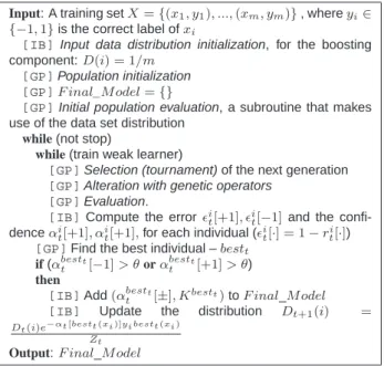
4.3. The InfoBoost GP learning algorithm
The steps of the learning process are presented in figure 2. Some steps are labeled[IB]or[GP], in order to
high-light which of the methods is “active” at that point. Input: A training setX={(x1, y1), ...,(xm, ym)}, whereyi∈
{−1,1}is the correct label ofxi
[IB]Input data distribution initialization, for the boosting
component:D(i) = 1/m
[GP]Population initialization
[GP]F inal_M odel={}
[GP]Initial population evaluation, a subroutine that makes
use of the data set distribution
while(not stop)
while(train weak learner)
[GP]Selection (tournament) of the next generation
[GP]Alteration with genetic operators
[GP]Evaluation.
[IB]Compute the errorǫi
t[+1], ǫit[−1]and the confi-denceαi
t[+1], αit[+1],for each individual (ǫit[·] = 1−rit[·]) [GP]Find the best individual –bestt
if(αbestt
t [−1]> θorα bestt
t [+1]> θ)
then
[IB]Add(αbestt
t [±], Kbestt)toF inal_M odel [IB] Update the distribution Dt+1(i) =
Dt(i)e−αt[bestt(xi)]yibestt(xi) Zt
Output:F inal_M odel
Figure 2. InfoBoost GP for Kernel Learning The basic idea consists of inserting boosting principles into the genetic algorithm that produces new kernels. We obtain a hybrid method that can be perceived as InfoBoost with GP as a weak learner.
Practically, the task is to train a classifier – an SVM with a proper kernel function – to distinguish between two classes, based on the information it can extract from a set of labeled samples X = {(x1, y1), ...,(xm, ym)} , where
yi∈ {−1,1}is the correct label ofxi.
The input data must be prepared to accept distribution variations during the learning process. Each instance will have an associated weight, which, at an intuitive level, ex-presses how difficult it is to properly classify that instance. Initially, no such information is available, so all instances have the same weight. The distribution is thus initialized withD(i) = 1/m.
The kernel function is evolved using genetic program-ming, a process that has several classic steps: the initializa-tion of the candidate soluinitializa-tion populainitializa-tion, the evaluainitializa-tion of the generated individuals on the initial distribution, the se-lection procedure for the current individuals, the alteration phase (using the genetic operators presented in section 4.1), and a reevaluation of the population according to the current distribution over the training data. The last three steps are repeated for a number of generations or until convergence (this is the stopping criterion in Figure 2).
The GP acts as a weak learner for InfoBoost on periods of consecutive iterations, during which the kernels are eval-uated on the same training subset. After this local training period, the kernel that performs best over the target distri-bution is chosen. The smallest tree is preferred in case of a
tie. If this individual’s quality, expressed as the confidence parameters (equations (6) and (7) from the InfoBoost sec-tion) is better than some thresholdθ, then this individual is accepted as a component of the final model. The distribu-tion is updated according to equadistribu-tion (4), considering the classification of the best individual.
4.4. Implementation details
Two open-source research tools were used in the imple-mentation: ECJ [18], a research Evolutionary Computing system written in Java, and LIBSVM [6, 11], an integrated software for support vector classification. In the former, a Boosted GP module was developed, extending the pro-vided basic elements for genetic programming problems, for defining the target problem, and customizing the input data, the tree nodes, and the fitness function. LIBSVM was extended in order to support custom kernels, integrated into the evolutionary computing platform, and called from the evaluation function in the kernel evolution process. Prelim-inary experimentation with the two support vector optimiza-tion methods provided by LIBSVM – C-SVM and nu-SVM – and various parameters for them, led to the choice of C-SVM withC= 1. In the next section, the results obtained with our method are compared to the results obtained using an RBF kernel, whose parameters were optimized by the brute-force grid search tool, also available in LIBSVM.
5. Results
The proposed method was tested on several databases for binary classification problems, available in the UCI ML Repository [10]:heart_scalewith 270 samples and 13 numeric features,breast_cancerwith 683 samples and 9 features, andwdbc, (Wisconsin Diagnostic Breast Can-cer), with 570 samples and 30 features.
Another test problem for our method was the classifica-tion of MSD domains.1 The domains – subsequences of amino-acids within the sequence of a protein, that carry out the function of the protein – can suffer significant structure modifications during evolution, while still conserving their function. Domains can be grouped in functional families, themselves divided in subfamilies. The MSD (Membrane Spanning Domains) super-family and some of its subfam-ilies show only little global-sequence conservation, hence alignment tools have a poor performance on recognizing such domains [21].
The protein domains database contains 1234 en-tries, each with 570 features. The representation of a protein
1This work is part of a project developed in collaboration with the
Databases and Machine Learning team at Laboratoire d’Informatique Fon-damentale, Université de Marseilles, France [5].
sequence is composed of theblastp[2] alignment scores with the positive proteins in the database.
For the tests, we used the following configuration:
pop_size= 70 individuals in each generation
tournament selection
mutation rate:p_m= 0.15
one node mutation rate:p_onm= 0.07 random number mutation rate:p_rnm= 0.01 crossover rate:p_c= 0.4
internal crossover rate:p_ic= 0.05.
The training set consisted of 88% percent of the data, while 12% were left for testing. 4-fold-cross-validation was performed at the evaluation of each individual kernel.
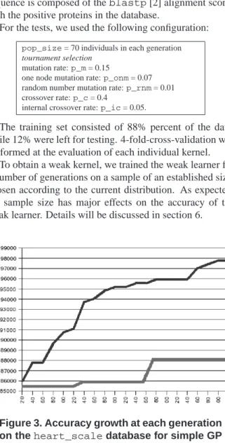
To obtain a weak kernel, we trained the weak learner for a number of generations on a sample of an established size, chosen according to the current distribution. As expected, the sample size has major effects on the accuracy of the weak learner. Details will be discussed in section 6.
Figure 3. Accuracy growth at each generation on theheart_scaledatabase for simple GP and InfoBoosted GP
Database heart_scale
Generations 20/600
Samples 150/216
Final training accuracy
with InfoBoosted kernel 100% Final validation accuracy
with InfoBoosted kernel 81% Best RBF training accuracy 100% Best RBF validation accuracy 54%
Table 1. Results onheart_scale
6. Discussion
Training error. When comparing the evolution of the best individual in a boosted GP, in relation with a pure GP,
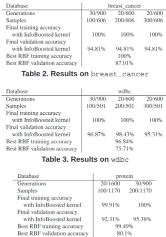
Database breast_cancer Generations 30/900 20/600 20/600
Samples 100/606 200/606 300/606
Final training accuracy
with InfoBoosted kernel 100% 100% 100% Final validation accuracy
with InfoBoosted kernel 94.81% 94.81% 94.81% Best RBF training accuracy 100%
Best RBF validation accuracy 87.01%
Table 2. Results onbreast_cancer
Database wdbc
Generations 30/900 20/600 20/600
Samples 100/501 200/501 300/501
Final training accuracy
with InfoBoosted kernel 100% 100% 100% Final validation accuracy
with InfoBoosted kernel 96.87% 98.43% 95.31% Best RBF training accuracy 96.84%
Best RBF validation accuracy 75.71%
Table 3. Results onwdbc
Database protein
Generations 20/1600 30/900
Samples 100/1170 200/1170
Final training accuracy
with InfoBoosted kernel 99.91% 100% Final validation accuracy
with InfoBoosted kernel 92.31% 95.38% Best RBF training accuracy 99.49% Best RBF validation accuracy 80.1%
Table 4. Results onprotein domains
we notice a slight improvement tendency for the pure GP method, and a more pronounced growth of the accuracy in the boosted process (figure 3).
Generalization error. Often, with sufficient boosting rounds, on noise-less data, the training error will eventu-ally reach zero, or a value close to zero. Such cases are not necessarily good, since they may result from overfitting the training data. Even with the encouragement of shorter ker-nels, the weak classifiers may be tempted to explain in detail the training data, but eventually unable to generalize, and thus perform poorly on unseen data. We notice that the ge-neralization error is, as expected, strongly dependent on the training sample size. Sacrificing time efficiency, we should provide reasonably large samples to the weak learner, in or-der to obtain good results on generalization.
A small sample results in an apparently good weak ker-nel with respect to the training subset, but overfitted, and with poor performance when integrated in the final model and tested against the entire data set. Using small samples results in many kernels identifying only small chunks of data, until all the training instances have been covered by at least one such kernel.
On the other hand, larger samples tend to reduce the
ge-Samples 16 200 300 500
Validation accuracy 93.75% 98.43% 95.31% 84.37%
Table 5. Validation accuracy with different sample sizes, on thewdbcdatabase
neralization capability of the learned SVM. Forcing the ge-neralization on a very large dataset, the opposite effect is obtained, by promoting kernels whose corresponding hy-perplane is obtained from most of the instances as support vectors, and which perfectly “surrounds” the given samples. Table 5 illustrates these statements on thewdbcdatabase. We note that regardless of the sample size, the training ac-curacy was 100%.
Support vector machines trained with RBF kernels ex-pose large variations for the training error / validation er-ror ratio. If the SVM is forced to achieve high accuracy on the training data, the accuracy on the validation set may decrease drastically. For example, on theheart_scale database, the validation error can reach 46% for 0% training errors, and a 6% validation error for a 2% training error. Results versus time. The results exposed in this section support the choice of a kernel learned from the data. How-ever, this is not a good option in case a very quick answer is needed. The accuracy is indeed significantly boosted, but the run time (on an AMD64 CPU, 1.8GHz) varies from tens of minutes to several hours, depending on the complexity of the problem.
7. Conclusions and future work
This paper discussed the necessity of learning inter-instance similarities from data in the context of non-trivial classification tasks and presented a method for learning ker-nel functions that can be used in non-linear SVM classifi-cation. We propose a method that uses genetic program-ming to evolve a kernel function as an additive or multi-plicative combination of linear, polynomial and RBF ker-nels. A boosting-like procedure, inspired from InfoBoost, is used to help the evolved kernels concentrate on the most difficult objects to classify.
Comparing the results obtained using our method on one side and the results obtained by SVMs employing RBF ker-nels or kerker-nels evolved by simple GP on the other side, we find a lower training and generalization error for the form-ers. Moreover, we noticed that the boosting component is indeed effective, since the generalization error tends to de-crease at each boosting round, along with the training error. Future work includes some enhancements of the current method and the development of more advanced methods for the chosen problem. So far, only 2-class problems were
approached with the proposed method. A multiclass version needs to be adapted and tested.
Some scalability issues must also be taken into account. The learning process is complex, involving a costly evo-lutionary algorithm, with sufficiently many generations so that it can allow the individuals to discover and adapt to the difficult instance set, and an even more time expensive SVM training process for the evaluation of each individual. Another – more complex – direction concerns the pos-sibility of designing kernels that have different expressions for different areas of the instance space. A kernel func-tion’s value gives some similarity measure for its two argu-ments. In general, distance or similarity functions tend to be considered the same in the entire space. However, practice shows that some subspaces may have different properties, making it difficult to find a general rule. Therefore, the pos-sibility of defining kernels whose expression captures the local particularities of the space, instead of trying to approx-imate them in a general expression, should be explored.
References
[1] M. Aizerman, E. Braverman, and L. Rozonoer. Theoret-ical foundations of the potential function method in pat-tern recognition learning. Automation and Remote Control, 25(821-837):17, 1964.
[2] S. Altschul, W. Gish, W. Miller, E. Myers, and D. Lipman. Basic local alignment search tool. J. Mol. Biol, 215(3):403– 410, 1990.
[3] J. A. Aslam. Improving algorithms for boosting. In COLT
’00: Proceedings of the Thirteenth Annual Conference on Computational Learning Theory, pages 200–207, San
Fran-cisco, CA, USA, 2000. Morgan Kaufmann Publishers Inc. [4] B. Boser, I. Guyon, and V. Vapnik. A training algorithm for
optimal margin classifiers. Proceedings of the fifth annual
workshop on Computational learning theory, pages 144–
152, 1992.
[5] C. Capponi, G. Fichant, Y. Quentin, and F. Denis. Classi-fication of Domains with Boosted Blast. Technical report, LIF, 2005.
[6] C. Chang and C. Lin. LIBSVM: a library for support vector machines, software available at:
www.csie.ntu.edu.tw/∼cjlin/libsvm, 2001. [7] N. Cristianini and J. Shawe-Taylor. An Introduction to
Support Vector Machines and Other Kernel-based Learning Methods. Cambridge University Press, 2000.
[8] L. Dio¸san and M. Oltean. Evolving kernel function for sup-port vector machines. In C. C., editor, The 17th European
Conference on Artificial Intelligence, Evolutionary Compu-tation Workshop, pages 11–16, 2006.
[9] L. Dio¸san, M. Oltean, A. Rogozan, and J. P. Pecuchet. Ge-netically designed multiple-kernels for improving the SVM performance. In GECCO 2007. ACM, 2007.
[10] D.J. Newman, S. Hettich, C.L. Blake and C.J. Merz. UCI Repository of machine learning databases, 1998.
[11] R. Fan, P. Chen, and C. Lin. Working Set Selection Using Second Order Information for Training Support Vector Ma-chines. The Journal of Machine Learning Research, 6:1889– 1918, 2005.
[12] Y. Freund and R. Schapire. Experiments with a new boost-ing algorithm. Machine Learnboost-ing: Proceedboost-ings of the
Thir-teenth International Conference, 148:156, 1996.
[13] Y. Freund and R. Schapire. A decision-theoretic generaliza-tion of on-line learning and an applicageneraliza-tion to boosting.
Jour-nal of Computer and System Sciences, 55(1):119–139, 1997.
[14] T. Hertz, A. Hillel, and D. Weinshall. Learning a kernel function for classification with small training samples.
Pro-ceedings of the 23rd international conference on Machine learning, pages 401–408, 2006.
[15] H. Iba. Bagging, boosting, and bloating in genetic program-ming. Proceedings of the Genetic and Evolutionary
Compu-tation Conference, 2:1053–1060, 1999.
[16] J. Koza. Genetic programming: on the programming of
com-puters by means of natural selection. MIT Press Cambridge,
MA, USA, 1992.
[17] W. Langdon and B. Buxton. Genetic programming for com-bining classifiers. Proceedings of GECCO-2001, pages 66– 73, 2001.
[18] S. Luke, L. Panait, G. Balan, Z. Skolicki, J. Bassett, R. Hubley, and A. Chircop. ECJ: A Java-based evolution-ary computation and genetic programming research system,
http://cs.gmu.edu/∼eclab/projects/ecj/ .
[19] J. Mercer. Functions of positive and negative type and their
connection with the theory of integral equations. Philos.
Trans. Roy. Soc. London, 1909.
[20] G. Paris, D. Robilliard, and C. Fonlupt. Applying Boost-ing Techniques to Genetic ProgrammBoost-ing. Artificial
Evolu-tion 5th InternaEvolu-tional Conference, EvoluEvolu-tion Artificielle, EA,
2310:267–278, 2001.
[21] Y. Quentin, J. Chabalier, and G. Fichant. Strategies for the identification, the assembly and the classification of integrated biological systems in completely sequenced genomes. Comput Chem, 26(5):447–57, 2002.
[22] R. Schapire. The boosting approach to machine learning: An overview. MSRI Workshop on Nonlinear Estimation and
Classification, 2002.
[23] B. Schölkopf, A. Smola, C. Burges, and R. Soentpiet.
Ad-vances in Kernel Methods: support vector learning. MIT
Press, 1999.
[24] N. Shental, A. Bar-Hillel, T. Hertz, and D. Weinshall. Com-puting Gaussian mixture models with EM using equivalence constraints. Advances in Neural Information Processing Systems, 16:465–472, 2004.
[25] B. K. Tanasanee Phienthrakul. Evolutionary strategies for multi-scale radial basis function kernels in Support Vector Machines. In GECCO’05, pages 905–911, 2005.
[26] V. Vapnik. Statistical learning theory. Wiley, 1998. [27] V. Vapnik and A. Lerner. Pattern recognition using
gener-alized portrait method. Automation and Remote Control, 24(3):774–780, 1963.