c
⃝T ¨UB˙ITAK
doi:10.3906/elk-1311-58 h t t p : / / j o u r n a l s . t u b i t a k . g o v . t r / e l e k t r i k /
Research Article
Gender classification: a convolutional neural network approach
Shan Sung LIEW1,∗, Mohamed KHALIL-HANI1, Syafeeza AHMAD RADZI2,Rabia BAKHTERI1
1VeCAD Research Laboratory, Faculty of Electrical Engineering, Universiti Teknologi Malaysia, Skudai, Johor, Malaysia
2FKEKK, Universiti Teknikal Malaysia Melaka, Hang Tuah Jaya, Durian Tunggal, Melaka, Malaysia Received: 07.11.2013 • Accepted/Published Online: 25.02.2014 • Final Version: 23.03.2016
Abstract: An approach using a convolutional neural network (CNN) is proposed for real-time gender classification based on facial images. The proposed CNN architecture exhibits a much reduced design complexity when compared with other CNN solutions applied in pattern recognition. The number of processing layers in the CNN is reduced to only four by fusing the convolutional and subsampling layers. Unlike in conventional CNNs, we replace the convolution operation with cross-correlation, hence reducing the computational load. The network is trained using a second-order backpropagation learning algorithm with annealed global learning rates. Performance evaluation of the proposed CNN solution is conducted on two publicly available face databases of SUMS and AT&T. We achieve classification accuracies of 98.75% and 99.38% on the SUMS and AT&T databases, respectively. The neural network is able to process and classify a 32 × 32 pixel face image in less than 0.27 ms, which corresponds to a very high throughput of over 3700 images per second. Training converges within less than 20 epochs. These results correspond to a superior classification performance, verifying that the proposed CNN is an effective real-time solution for gender recognition.
Key words: Gender classification, convolutional neural network, fused convolutional and subsampling layers, backprop-agation
1. Introduction
Gender classification was first perceived as an issue in psychophysical studies; it focuses on the efforts of understanding human visual processing and identifying key features used to categorize between male and female individuals [1]. Research has shown that the disparity between facial masculinity and femininity can be utilized to improve performances of face recognition applications in biometrics, human–computer interactions, surveillance, and computer vision. However, in a real-world environment, the challenge is how to deal with the facial image being affected by the variance in factors such as illumination, pose, facial expression, occlusion, background information, and noise. This is then also the challenge in the development of a robust face-based gender classification system that has high classification accuracy and real-time performance.
The conventional approach applied in face recognition, including face-based gender recognition, typically involves the stages of image acquisition and processing, dimensionality reduction, feature extraction, and classification, in that order. Prior knowledge of the application domain is required to determine the best feature extractor to design. In addition, the performance of the recognition system is highly dependent on the type of classifier chosen, which is in turn dependent on the feature extraction method applied. It is difficult
to find a classifier that combines best with the chosen feature extractor such that an optimal classification performance is achieved. Any changes to the problem domain require a complete redesign of the system.
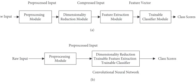
The convolutional neural network (CNN) is a neural network variant that consists of a number of convolutional layers alternating with subsampling layers and ends with one or more fully connected layers in the standard multilayer perceptron (MLP). A significant advantage of the CNN over conventional approaches in pattern recognition is its ability to simultaneously extract features, reduce data dimensionality, and classify in one network structure. Such a structure, as illustrated in Figure 1, can boost recognition accuracy efficiently and cost-effectively.
Raw Input Preprocessing
Module
Trainable
Classifier Module Class Scores Feature Extraction Module Feature Vector Dimensionality Reduction Module Compressed Input Preprocessed Input (a)
Raw Input Preprocessing
Module Class Scores
Preprocessed Input
Convolutional Neural Network Dimensionality Reduction Trainable Feature Extraction
Trainable Classifier
(b)
Figure 1. Pattern recognition approaches: (a) conventional, (b) CNN-based.
The CNN performs both feature extraction and classification within a single network structure through learning on data samples [4]. Feature selection is also integrated into the training process by learning the weights held responsible for extracting features [2]. The CNN also has the ability to extract topological properties from a raw input image with no or minimal preprocessing required [2]. In addition, a certain degree of invariance is achieved while preserving the spatial topology of input data [1]. The CNN also provides partial resistance and robustness to geometric distortions and transformations, and other 2D shape variations [2]. Hence, the CNN is specifically designed to cope with shortcomings of the traditional feature extractor that is characterized by being static, is designed independently of the trainable classifier, and is not part of training procedure [3]. A final benefit of CNNs is that they are relatively easier to train since they have fewer parameters than fully connected MLP neural networks with the same number of hidden layers. Consequently, the CNN has shown promising success in a wide range of applications that include character recognition [4], face recognition [5], human tracking [6], traffic sign recognition, and many others.
In this paper, we propose a novel approach for real-time gender classification using a CNN. The main contributions of this research are as follows. First, an efficient and effective 4-layer CNN for real-time face-based gender classification is proposed. The network architecture has a reduced design complexity with a smaller number of layers, neurons, trainable parameters, and connections when compared with existing methods. We apply a novel algorithm in fusing the convolutional and subsampling layers, and we replace the convolution operation with cross-correlation (i.e. we do not perform flipping of weights in the kernel matrix, as required in convolution). Second, we conduct experiments to study and verify that the application of cross-correlation
instead of convolution not only does not harm but actually improves the performance of the CNN in terms of classification rate and processing speed. To the best of our knowledge, this appears to be the first time this aspect of the design is reported in the literature. Finally, we benchmark our CNN solution for gender recognition on two different face databases of SUMS and AT&T, and results show that the proposed method outperforms almost all previous methods.
The remainder of this paper is organized as follows. Section 2 discusses previous works on gender classification. Section 3 describes the background of the classical CNN. A detailed discussion on the architecture and algorithms of the proposed automatic gender recognition system is presented in Section 4. Experimental work and results are provided in Section 5, and Section 6 concludes the work done and proposes recommendations for future works.
2. Previous work
Although gender classification can play a significant role in many computer vision applications, it has not been as well studied compared to the more popular problem of recognition and identification. Most of the existing solutions for pattern recognition problems apply trainable or nontrainable classifiers preceded by heuristic-based feature extractors. This section briefly discusses previous works from the perspective of the classification methods applied.
The support vector machine (SVM) is a popular algorithm for classification. In [7], a gender classification system using a local binary pattern (LBP) and SVM with polynomial kernel was proposed, in which the classification rate of 94.08% on the CAS-PEAL face database was reported. An average processing time of 0.12 s was achieved with MATLAB 6.1 implementation on a 3.0 GHz CPU. A disadvantage of the method is that high classification performance can only be achieved if the block size for the LBP operator is correctly selected, which is a rather difficult task. The work in [8] reported a high classification accuracy of 99.30% on the SUMS face database. This work applied Viola and Jones face detection, 2D-DCT feature extraction, and the K-means nearest neighbor (KNN) classifier. 2D-DCT is a compute-intensive algorithm; hence, this method is not suitable for real-time applications. Among the first attempts to apply neural networks in gender classification, one was reported in [9]. With a fully connected MLP used in conjunction with a large number of image processing modules, the average error rate was 8.1%, which is rather large compared to state-of-the-art results. The hybrid approach proposed in [10] processed the face image with principal component analysis (PCA) for dimensionality reduction. A genetic algorithm (GA) was then used to select a good subset of eigenfeatures. An average error rate of 11.30% was reported. In addition to the poor error rate achieved, the main drawback of this method is that, although it is an effective global random search method, the GA exhibits high computational complexity. The main disadvantages of the aforementioned methods are that the feature extraction and classification modules are designed and trained separately, and they require prior application-specific knowledge in order to obtain optimal preprocessing and feature extraction designs.
Among the first to propose gender classification by combining both feature extraction and classification in a single neural network were Titive and Bouzerdoum in [1]. Their technique, which applied a novel shunting inhibitory convolutional neural network (called SICoNNets), had an average classification accuracy of 97.1% on the FERET face database. The superior performance achieved was mainly due to a shunting inhibitory neuron that had two activation functions and one division to perform. In [5], the proposed CNN comprised six layers, with the final layer being a single neuron to represent the output class. On the FERET database, a classification rate of 94.7% was achieved on unmixed datasets. In short, the above CNN-based solutions demonstrate the potential of achieving superior performance in recognition problems and gender classification in particular.
3. Background on convolutional neural network
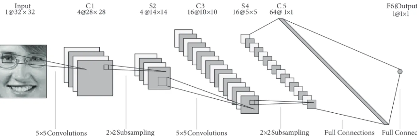
A CNN is a type of feedforward network structure that is formed by multiple layers of convolutional filters alternated with subsampling filters followed by fully connected layers. Figure 2 shows the classical LeNet-5 CNN, first introduced by LeCun et al. in [4], which is the basis of the design of conventional CNNs. In [4], it was successfully applied in a handwritten digit recognition problem. LeNet-5 has six processing layers, not including the input layer, which is of image size 32 × 32 pixels.
Input
1@32 × 32 4@28× 28C1 16@5×5S 4 64@ 1×1C 5
5×5Convolutions 5×5Convolutions Full Connections Full Connections
F6(Output) 1@1×1 S2
4 @14×14 16@10×10C3
2×2Subsampling 2×2Subsampling
Figure 2. Architecture of the classical LeNet-5 CNN.
As illustrated in Figure 2, the processing layers consist of three convolutional layers C1, C3, and C5 interspersed in between with two subsampling layers, S2 and S4, and an output layer, F6. The convolutional and subsampling layers are organized into planes called feature maps. Each neuron in a convolutional layer is connected locally to a small input region of size 5 × 5 (the receptive field) in the preceding layer [1]. All neurons from the same feature map receive inputs from different 5 × 5 input regions, such that the whole input plane is scanned, but they share the same set of weights (that forms the kernel). This is called local weight sharing; each feature map is the result of convolving the kernel with a receptive field. However, different feature maps in the same layer use different kernels. In the subsampling layers, the feature maps are spatially downsampled; that is, the map size is reduced by a factor of two. For example, the feature map in layer C1 of size 28 × 28 is subsampled to a corresponding feature map of size 14 × 14 in the subsequent layer S2. The output layer F6, which is a MLP, performs the classification process. The concepts of local receptive field, weight sharing, and spatial subsampling mentioned above are the three principle architectural ideas behind the design of a CNN [2,6]. In weight sharing topology, all neurons in a feature map use the same incoming set of weights (kernel weights), and feature extraction is performed by convolving the image with these kernels [3,11]. As such, a feature map in a CNN is a 2D representation of extracted features from input feature map(s) or input image. Such an arrangement of neurons with identical kernel weights and local receptive fields in a spatial array forms an architecture akin to models of biological vision systems. There are several advantages of this strategy. First, the network complexity and the dimensionality of data are reduced effectively [1,11]. Weight sharing also serves as an alternative to weight elimination, which reduces the memory capacity of the machine. In the CNN, subsampling is applied for the purpose of dimensionality reduction while still maintaining relevant information in the input plane, as well as to reduce shift and distortion sensibility of detected features [3]. For more details on the algorithms of the LeNet-5 CNN, please refer to [4].
4. Proposed CNN for gender classification
In this section, we present the design details of the proposed CNN for automatic gender recognition. We describe the network architecture, provide the corresponding formulations and algorithms, and present the training algorithm of our CNN.
4.1. Architecture
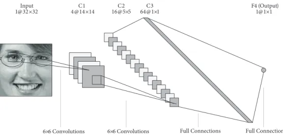
Figure 3 shows the overview of the network architecture of our CNN. The network consists of four processing layers: three convolutional layers (denoted by C1, C2, and C3) and one output layer (denoted by F4). The input layer is a 2D face image of size 32 × 32 pixels. Layers C1, C2, and C3 are convolutional layers of four 14 × 14, sixteen 5 × 5, and sixty-four 1 × 1 feature maps, respectively. Layer F4 consists of a single perceptron, also referred as a 1 @ 1 × 1 map.
Input 1@32×32 C1 4 @14×14 C2 16@5×5 C3 64@1×1
6×6 Convolutions 6×6 Convolutions Full Connections Full Connections
F4 (Output) 1@1×1
Figure 3. Proposed CNN architecture for gender classification.
To connect the feature maps of layer C1 to the subsequent layer C2, we apply the partial-connection scheme provided in Figure 4. This connection, not being a full connection, essentially forces each filter to learn different features from the same feature map [4]. On the other hand, layers C2 and C3 are fully connected: each neuron in C3 (which is a 1 × 1 map) is connected to a 5 × 5 region in all 16 feature maps in C2.
0 2 1 3 C1 × × × × 0 × 1 × 2 × 3 × 4 × × 5 × × 6 × × 7 × × 8 × × × 9 × × × 10 × × × 11 × × × 12 C2 × × 13 × × 14 × × × × 15
4.2. Formulation: fusion of convolutional and subsampling layers
The number of layers of the proposed CNN is reduced by fusing a convolutional and a subsampling layer into one layer. The idea was first introduced by Simard et al. [12], which was later refined by Mamalet and Garcia [13]. In this work, we replace consecutive convolutional and subsampling layers with one convolutional layer using strides of 2. A feature map, Yj(l)(x , y) in layer l can be described by the following equation:
Yj(l)(x , y) = f ∑N i= 0 K(l) x ∑ u= 0 K∑y(l) v= 0 Yi(l−1) ( S(l)x x +u, S(l)y y +v ) wji(l)(u, v) + θ(l)j , (1)
where Yi(l−1) andYj(l) are the input and output feature maps respectively,f( ) denotes the activation function,
w(l)ji is the convolutional kernel weight, θj(l) is the bias, N represents the total number of input feature maps,
S(l)x is the horizontal convolution step size, S (l)
y is the vertical convolution step size, andK (l)
x and K
(l)
y are the width and height of convolutional kernels, respectively. The width W(l) and height H(l) of the output feature map with convolution step sizes of Sx(l) and S
(l)
y can be computed as:
W(l) = W (l−1) −K(l) x Sx(l) + 1 (2) and H(l) = H (l−1) − K(l) y Sy(l) + 1, (3)
where W(l−1) and H(l−1) correspond to the width and height of input feature map.
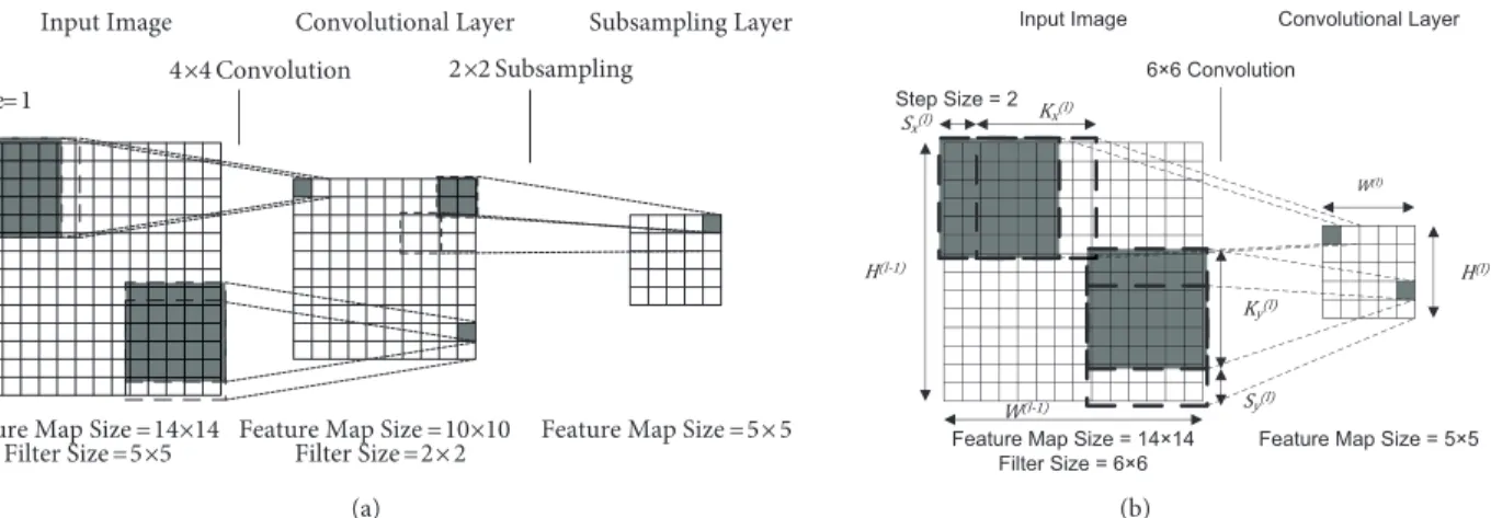
Figure 5 gives a pictorial representation of the formulation above. The diagram shows that a 5 × 5 convolution followed by a 2 ×2 subsampling operation can be replaced by a single 6 ×6 convolution operation with step size (strides) of 2, because they generate exactly the same output feature map.
4×4 Convolution 2×2 Subsampling
Feature Map Size =14×14
Filter Size =5×5 Feature Map Size =10×10Filter Size =2× 2 Feature Map Size =5× 5
Input Image Convolutional Layer Subsampling Layer
Step Size =1
(a) (b)
6×6 Convolution
Feature Map Size = 14×14 Filter Size = 6×6
Feature Map Size = 5×5 Input Image Convolutional Layer
Step Size = 2
Figure 5. Operations on feature maps in the convolutional layer: (a) conventional approach applying convolution (with step size of 1) followed by subsampling, (b) fused convolution/subsampling approach applying convolutions with step size of 2.
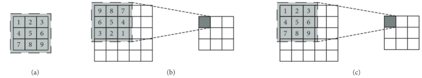
Note that, in the formulation given above, we perform cross-correlation instead of convolution. Recall that in image processing, convolution and cross-correlation perform similar functions, except that in the convolution process, the kernel weights are flipped vertically and horizontally. The general equation for a 2D discrete convolution is given by:
Y(x , y) = Kx ∑ u= 0 Ky ∑ v= 0 X(x −u, y −v)w(u , v) (4)
where X is an input image, Y is the output image, w is the kernel, and Kx and Ky represent the width and height of convolutional kernel, respectively. This operation involves flipping of the kernel weights before the dot product is performed. In contrast, a 2D discrete cross-correlation (for image processing) is described by the following equation: Y(x , y) = Kx ∑ u= 0 Ky ∑ v= 0 X(x +u , y +v)w(u , v). (5)
Essentially, Eqs. (4) and (5) are similar, except in Eq. (5), the kernel weights are not flipped. We illustrate these operations using the diagrams in Figure 6, where Figure 6a gives an example convolution kernel. In the conventional approach, as depicted in Figure 6b, a 2D discrete convolution is performed by convolving an overlapped input plane with the convolution kernel with kernel weights being flipped in both horizontal and vertical directions. In Figure 6c, the same operation is shown, but now without flipping the kernel. Since values of the convolution kernel (weights) in a convolutional layer are randomly initialized, flipping has little effect on the convolution output.
9 8 7 6 5 4 3 2 1 1 2 3 4 5 6 7 8 9 1 2 3 4 5 6 7 8 9 (a) (b) (c)
Figure 6. The 2D discrete convolution operation: (a) example convolution kernel, (b) convolution with kernel weights flipped, (c) convolution with kernel weight not flipped.
Flipping operations add more computational time in both feedforward and backward propagations. Hence, the modification of replacing convolution with cross-correlation is advantageous, especially when dealing with numerous convolutions to be performed on large kernel sizes, and on large datasets within a large number of training iterations (epochs).
In this work, we apply, in the convolutional layers, a scaled hyperbolic tangent function as described by the following equation:
f(x) =Atanh (Bx), (6)
where A denotes the amplitude of the function and B determines its slopes at the origin. The values of A and B are set at 1.7159 and 2/3 as suggested by LeCun et al. [4].
The value at output neuron in F4 is given by the following equation: Yj(l) = f ( N ∑ i= 1 Yi(l−1)w(l)ji + θ(l)j ) , (7)
where f( ) represents the activation function used for each neuron, N is the total number of input neuron(s),
Yi(l−1) is the value of the input neuron, w(l)ji is the synaptic weight connecting the input neuron(s) to the output neuron, and θ(l)j denotes the bias. Male gender is represented by the output value of +1 , whereas −1 indicates that the pattern belongs to the female class.
Table 1. Comparison of backpropagation algorithm complexity between that of the conventional CNN and that of the architecture with fused convolutional and subsampling layer [13].
Layer Number of operations
Convolutional layer, Ci WiHiKi2 Subsampling layerSi WiHiKi2+ 1 4 F used layerCSi ( 4 (Ki + 1) 2 + (Ki+ 1 + 1) 2)WiHi 16 Speedup f actor, (Ci,S) CSi 16K2 i+ 4K2i+ 1 4(Ki+ 1)2+ (Ki+ 1+ 1)2
Table 1 shows the comparison of complexity in the backpropagation training algorithm when applied in the conventional CNN architecture and the CNN with fused convolutional/subsampling layers [10]. It can be observed that the fused convolutional layer can achieve higher computational speeds compared to the combination of a convolutional layer and subsampling layer, as in conventional CNN architecture.
In addition to the performance speedup gained as a result of a fused convolutional layer, we also observe a positive effect on the classification performance when weight flipping is not applied. This is discussed later in Section 5. It should be noted here that researchers, for example in [14] and [15], have applied cross-correlation instead of convolution in the convolutional layers, although they have stated in their papers that convolution is performed.
4.3. Training algorithm
Backpropagation is the most common learning method for neural networks. Error gradients are computed and propagated from output to input layers, and the weight values are updated so as to minimize the network error. However, a major weakness of standard backpropagation is its extremely slow convergence rate. In second-order methods, adjustments to learning rate parameters are performed dynamically to accelerate network convergence. In this paper, we apply a second-order backpropagation algorithm, the stochastic diagonal Levenberg–Marquardt (SDLM) algorithm, that was proposed by LeCun et al. in [16]. We enhance the method by adding an annealed global learning rate for faster network convergence. The algorithm below shows the training procedure of our CNN, using backpropagation with the SDLM algorithm as a learning mechanism.
In InitializeWeight( ), the kernel weights are initialized with random values generated based on a uniform distribution within the range of [−0.05,0.05] . We have performed experiments using different weight initialization methods with different parameter values, and we have found that uniform distribution gives the best result.
Algorithm. Training procedure of CNN. 1: InitializeWeight (CNN);
2. while not reaching convergence do
3: CalculateLearningRateSDLM (samples);
4: Shuffle (samples);
5: for each training sample do
6: output ← ForwardPassCNN (sample); 7: loss ← CalculateError (output); 8: error ← BackwardPassCNN (loss);
9: WeightUpdate (error);
10: end for 11: end while
The SDLM algorithm approximates the Hessian matrix as a Jacobian square of network output error with respect to the weights. The approximation yields acceptable computational costs besides ensuring invertibility and a faster convergence rate [16]. In theCalculateLearningRateSDLM (samples)procedure, the SDLM learning algorithm is enhanced with annealed global learning rates. The adaptive learning rate for each individual weight (or biases) is computed using:
ηji = ϵ ⟨∂2Y ∂w2 ji⟩ +µ, (8)
where ηji is the learning rate for weight wji, ϵdenotes the annealed global learning rate, andµ is regularization parameter. Approximation of the 2nd derivative of the output with respect to the weight is computed from the following equation: ⟨∂2Y ∂w2 ji ⟩new = (1 −γ)⟨ ∂2Y ∂w2 ji ⟩old +γ⟨ ∂2Y ∂w2 ji ⟩current, (9)
where γ is a small memory constant that determines the influence of the previous value on the calculation of the next learning rate. The annealed global learning rate is given as
ϵt+ 1 = ϵmax t= 0 ϵmin ϵt< ϵmin ϵt ×α otherwise (10)
where α denotes the fading factor of the global learning rate,ϵmax is the initial global learning rate, and ϵmin is the minimum global learning rate. The calculations of learning rates are only performed once every two training epochs, and the parameters are set as follows: µ = 0.03 , γ = 0.00001 , ϵmax = 0.001 , ϵmin = 0.00001 , and α = 0.8 . Each individual weight or bias is updated with its corresponding learning rate.
In step 7 of the training procedure, the network error is determined. We use mean squared error (MSE) as the loss function, described by the following equation:
LP = 1
2(YP −DP) 2
, (11)
where DP denotes the desired output value for a particular pattern P, YP is the actual output value, and LP is the output of loss function, i.e. the MSE.
In step 9 of the training procedure, the kernel weights are updated. The weight updating is similar to that applied in standard backpropagation, except that, in this case, each individual weight (or bias) is updated
with its corresponding learning rate according to the following equations: wji(t+ 1) =wji(t)−ηji ∂YP ∂wji(t) , (12) θj(t+ 1) =θj(t)−ηj ∂YP ∂θj(t) , (13)
where wji(t+ 1) and θj(t+ 1) are the new weight and bias values for the next training iteration, respectively.
5. Experimental work and results
This section presents the experimental results of our CNN solution for gender classification. The proposed CNN algorithm is written in C, compiled using GCC as a single-threaded program with optimization level 3 (O3) in Ubuntu 12.04 LTS. Our CNN is implemented on an Intel Core 2 Duo T8300 (2.4 GHz) PC with 3 GB RAM. The code is also cross-compiled for execution on an Altera Nios II processor with 1 GB RAM and 280 MHz clock, and implemented on the Stratix III FPGA system-on-chip platform.
5.1. Databases and dataset preparation
The classification performance of the trained CNN is evaluated on two publicly available face databases of SUMS and AT&T. For performance evaluation and benchmarking, we apply our gender classification system on the SUMS face database. SUMS, or the Stanford Medical Student Face Database, consists of a total of 400 gray-scale images with a 200 × 200 sized image per subject. There are 200 male and 200 female subjects in the database. The faces are in upright, frontal position, with little or no variances in subject illumination. Subjects have different facial expressions (smiling/nonsmiling) and facial details (glasses/no glasses).
The AT&T face database, formerly known as the ORL database, contains 10 images of 40 subjects (36 males and 4 females), with original image size of 92 × 112 pixels. The images are taken on dark homogeneous backgrounds with slightly varying illumination, in which subjects’ faces are in an upright frontal position (with tolerance for some side movement). There are variations in face images in terms of facial expressions (open/closed eyes, smiling/nonsmiling) and facial details (glasses/no glasses).
The face images in the SUMS face database are manually cropped to contain only the main facial features: eyes, eyebrows, nose, mouth, and beard and glasses if present. They are then resized to 32×32 pixels. For the AT&T face database, manual cropping with window size of 92 × 92 pixels is performed on raw face images, which are then resized to 32 × 32 pixels. Examples of cropped images for the SUMS and AT&T databases are provided in Figures 7 and 8, respectively.
(a) (b)
Figure 7. Cropped face images in SUMS database: (a) male subjects, (b) female subjects.
The cropped face images are normalized using the local contrast normalization method. The pixel values are normalized to be within the range of −1 and +1 using the following equation:
x = (x− xmin) ( max−min xmax −xmin ) + min, (14)
where xis the input pixel value. xmax and xmin denote maximum and minimum pixel values in an input image, respectively. max is the upper boundary value, and min is the lower boundary value after normalization.
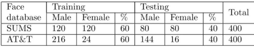
The preprocessed (cropped and normalized) images are divided randomly into training and testing sets, summarized as shown in Table 2. No images of the same subject exist in both training and testing sets.
Table 2. Training and testing sets of face databases.
Face Training Testing
Total
database Male Female % Male Female %
SUMS 120 120 60 80 80 40 400
AT&T 216 24 60 144 16 40 400
5.2. Results on classification performance
Figure 9 provides a visualization of the network outputs of a training image sample. Convolutions of input image in layer C1 extract 4 different complex features, which are convolved with 36 learned kernels to produce 16 simpler 5 × 5 features. These simpler features are then decomposed into a series of pixels representing output values of a fully connected layer and are finally classified through the output neuron. In this work, a white pixel represents the value of +1 , and −1 denotes a black pixel.
Since there are only two classes of pattern in gender recognition, the input pattern is classified as male if
YP ≥threshold, or female if otherwise. In this paper, the threshold value is set to 0. The number of correct classifications is obtained by presenting all the input patterns in the dataset to the network and accumulating all the correct classifications. The classification rate is then obtained by the following equation:
Classification rate = Correct classifications
Total testing samples ×100%. (15)
Figures 10a and 10b show the trends of the training and testing errors for the SUMS and AT&T datasets, respectively. It is observed that in the initial stage of the epoch, training MSEs are higher compared to corresponding testing MSEs, and they go lower after about 6 epochs. This can be explained by the fact that the number of samples in the training set is greater than the testing set. At a further stage in the training process, both training and testing errors are reduced to the extent that the values begin to stabilize. This indicates that the network is arriving at convergence. The effect of using the 2nd order method for network learning (i.e. SDLM) is clearly observed in the case of the SUMS database, implied by the steep gradient in the graph in Figure 10a.
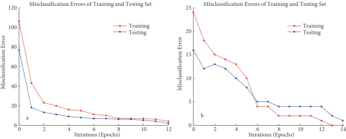
Figure 11 plots the misclassification error against epochs, showing that our CNN converges within 20 epochs of training iterations. We obtain a classification rate of 98.75% for the SUMS dataset and a high classification rate of 99.38% for AT&T face database. In the case of the AT&T dataset, only one misclassification is generated from 160 testing samples.
Figure 9. Feature maps at different layers of the CNN for a training image. 0 2 4 6 8 10 12 0.05 0.1 0.15 0.2 0.25 0.3 0.35 0.4 0.45 0.5
0.55 Mean Squared Errors (MSE) for Training and Testing
a Iterations (Epochs) Me an Squar ed Err or (MSE) Training Testing 0 2 4 6 8 10 12 14 0.04 0.06 0.08 0.1 0.12 0.14 0.16 0.18 0.2
0.22 Mean Squared Errors (MSE) for Training and Testing
b Iterations (Epochs) Me an Squar ed Err or (MSE) Training Testing
Figure 10. Training and testing errors for (a) SUMS, (b) AT&T database.
5.3. Evaluation of the effects of weight flipping to classification performance
In this paper, we have proposed a CNN architecture that performs cross-correlation in the fused convolutional layer instead of the standard 2D discrete convolution. We evaluate the effects of weight flipping in the convolution
kernels on the classification performance on both SUMS and AT&T face databases. The same learning method with the same parameter values was applied in both cases. Table 3 gives the results of this experiment. We achieve a significant increase of 1.87% in the classification rate in the case of SUMS. The same result is observed with the AT&T database, where the classification performance improves from 97.50% to 99.38%. This result proves that using cross-correlation (no weight flipping) instead of convolution (kernel weights are flipped) improves the classification performance of our CNN.
0 2 4 6 8 10 12 0 20 40 60 80 100
120 Misclassification Errors of Training and Testing Set
a Iterations (Epochs) Mis cl assi fica tion Error Training Testing 0 2 4 6 8 10 12 14 0 5 10 15 20
25 Misclassification Errors of Training and Testing Set
b Iterations (Epochs) Mis cl assi fica tion Error Training Testing
Figure 11. Misclassification errors for (a) SUMS database, (b) AT&T database. Table 3. Effect of weight flipping on CNN classification rates.
CNN convolutional layer applying: Classification rate (%)
SUMS AT&T Convolution (i.e. kernel weights are flipped) 96.88 97.50 Cross-correlation (i.e. kernel weights are not flipped) 98.75 99.38
5.4. Benchmarking results on classification performance
Tables 4 and 5 provide the results of benchmarking the proposed CNN against state-of-the-art previous works that were evaluated on the SUMS and AT&T databases, respectively. In the case of SUMS, we achieve a classification rate that is among the highest, second only to that of Nazir et al. in [7], in which they applied DCT with a Kohonen neural network. We can explain this by the fact that we did not apply histogram equalization to the cropped face images as this will eliminate the effects of illumination variations.
Table 4. Benchmarking results based on SUMS face database.
Researcher(s) Year Method(s) Classification rate (%)
Khan et al. [17] 2013 Decision tree 98.50
Majid et al. [18] 2003 DCT + modified KNN 98.54
Nazir et al. [8] 2010 DCT + KNN 99.30
Proposed work 2014 CNN with fused convolution and subsampling layers 98.75
Table 5 shows previous related works on gender classification using the AT&T face database. To the best of our knowledge, our proposed method achieves the highest classification rate among all other techniques
proposed in these papers. This shows the superior performance of the CNN over other feature extraction and classification methods.
Table 5. Benchmarking results based on AT&T face database.
Researcher(s) Year Method(s) Classification rate (%)
Jiao et al. [19] 2012 PCA + extreme learning machine 93.75
Basha et al. [20] 2012 Continuous wavelet transform & SVM 98.00
Berbar [21] 2013 DCT + SVM 98.93
Proposed work 2014 CNN with fused convolution and subsampling layers 99.38
5.5. Evaluation of training performance
We compare the training performance of the proposed method against LeNet-5 representing all conventional CNNs. Table 6 gives the number of trainable parameters and connections for the two cases. It is observed that our CNN has a slightly higher number of trainable parameters, with a small overhead of only 1.5%, as compared to the conventional architecture. However, in terms of the number of connections, the conventional CNN has 2.3 times more connections than the proposed CNN. Increasing the number of learnable parameters contributes to more memory space required, but more connections will create more computational load, thus slowing down the network.
Table 6. Summary of comparisons between 2 different architectures.
CNN architecture Total trainable parameters Total connections
LeNet-5 26789 207,745
Proposed CNN 27189 88,997
We measure the performances of different CNN architectures by evaluating the average processing time needed for each of them. The average processing times for a single training epoch with 240 and 480 training patterns, 10 training epochs, and testing of a single pattern are measured, respectively. The performance is evaluated without taking into account the time taken for weight initialization and reading input images from memory.
10 Epochs 1 Epoch (Double Dataset Size) 1 Epoch 0 5 10 15 20 25 30 35 40 45 Average Processing Time (s)
Training Performances of Different CNN Architectures
a b
Figure 12 provides the processing times of LeNet-5 and our CNN with and without convolution weight flipping. We observe that the proposed CNN requires the lowest processing time. Training the network for one epoch in CNN1 (LeNet5 with weight flipping in kernels) consumes about 4.65 s, while CNN4 (our CNN without weight flipping) requires only 1.98 s. CNN3 (our CNN with weight flipping) performs training of an epoch within 2.02 s, which implies that the effect of weight flipping is not very significant in slowing down the network for a single training epoch. However, the differences are amplified for more training epochs and with larger datasets to be learned. The difference of processing times in CNN3 and CNN4 trained within 10 epochs is 0.64 s. Similar patterns are observed as well in the FPGA platform. It is worth mentioning that the training of the face database is completed within less than 15 epochs, which is less than 1 min.
Figure 13 illustrates the significant speedup obtained on a PC platform compared to the FPGA platform, which is most probably due to hardware resource constraints on the second platform.
Without O3 Optimization With O3 Optimization 0 0.5 1 1.5 2 2.5x 10 5
Average Processing Time (s)
Average Processing Time for 1 Testing Epoch
a
Without O3 Optimization With O3 Optimization 0 100 200 300 400 500 600 Ave
rage Processing Time (ms)
Average Processing Time for 1 Testing Epoch
b
LeNet−5 with weight flip (CNN1) LeNet−5 without weight flip (CNN2) Simplified CNN with weight flip (CNN3) Simplified CNN without weight flip (CNN4)
Figure 13. Average processing time for a testing epoch running on (a) FPGA platform, (b) PC platform.
0 0.1 0.2 0.3 0.4 0.5 0.6 0.7
Average Processing Time (ms)
Average Processing Time for 1 Single Sample
0 0.2 0.4 0.6 0.8 1 1.2 1.4
Average Processing Time (s)
Average Processing Time for 1 Single Sample LeNet−5 with weight flip (CNN1) LeNet−5 without weight flip (CNN2) Simplified CNN with weight flip (CNN3) Simplified CNN without weight flip (CNN4)
a b
Figure 14. Average processing time for a single face image running on (a) PC platform, (b) FPGA platform.
In fact, in real-world applications, end users are more concerned with the classification time required for a single input pattern, rather than total training time needed for the network to learn all the training patterns.
Figure 14 shows the amount of processing time required for evaluation of a single test pattern. The figure clearly illustrates that the proposed CNN achieves significant speedup compared to LeNet-5, that is, 2.27 times faster than the conventional architecture. In addition, the effect of weight flipping in the testing phase is obviously seen as well. Our CNN without weight flipping performs 1.59 times faster than the one with weight flipping operations. In this experiment, CNN4 achieves an average processing time of less than 0.27 ms for a single sample. In other words, the proposed method is able to process more than 3700 3 input images of 2 × 32 pixels within 1 s, which is very suitable for implementation in a real-time platform.
6. Conclusion and future works
We have proposed an optimized CNN architecture for gender classification. The architecture consists of fused convolutional and subsampling layers, and cross-correlation is applied in the processing layers instead of convolution. Benchmarking results have shown that the proposed CNN has superior classification performance, achieving 98.75% and 99.38% classification rates on the SUMS and AT&T face databases respectively. In addition, our proposed architecture has achieved significant speedup, able to process and classify a 32 × 32 pixel input image in less than 0.3 ms on PC platform. To the best of our knowledge, this is among the first experiments to study the effect of weight flipping on the performance of a CNN in terms of classification rate and processing speed. The research work can be extended for face detection and alignment tasks using similar CNN architectures to produce a complete gender recognition system. The method is suitable for custom hardware implementation targeted for real-time processing in resource-constrained environments.
Acknowledgments
The authors would like to thank the Stanford University School of Medicine and AT&T Laboratories, Cam-bridge, for compiling and maintaining the face databases. This work was supported by the Ministry of Science, Technology and Innovation of Malaysia (MOSTI) and Universiti Teknologi Malaysia (UTM) under the eScience-Fund Grant No. 4S116.
References
[1] Tivive FHC, Bouzerdoum A. A gender recognition system using shunting inhibitory convolutional neural networks. In: International Joint Conference on Neural Networks; 2006; Vancouver, Canada. New York, NY, USA: IEEE. pp. 5336–5341.
[2] Khalajzadeh H, Mansouri M, Teshnehlab M. Face recognition using convolutional neural network and simple logistic classifier. Stud Comp Intell 2013; 223: 197–207.
[3] Strigl D, Kofler K, Podlipnig S. Performance and scalability of GPU-based convolutional neural networks. In: 18th
Euromicro International Conference on Parallel, Distributed and Network-Based Processing; 17–19 February 2010; Pisa, Italy. New York, NY, USA: IEEE. pp. 317–324.
[4] LeCun Y, Bottou L, Bengio Y, Haffner. P. Gradient-based learning applied to document recognition. P IEEE 1998; 86: 2278–2324.
[5] Duffner S. Face Image Analysis with Convolutional Neural Networks. Munich, Germany: GRIN Verlag, 2009. [6] Fan J, Wei X, Ying W, Yihong G. Human tracking using convolutional neural networks. IEEE T Neural Networ
2010; 21: 1610–1623.
[7] Lian HC, Lu BL. Multi-view gender classification using local binary patterns and support vector machines. Lect
[8] Nazir M, Ishtiaq M, Batool A, Jaffar MA, Mirza AM. Feature selection for efficient gender classification. In: Proceedings of the 11th WSEAS International Conference; 2010. pp. 70–75.
[9] Golomb BA, Lawrence DT, Sejnowski TJ. SEXNET: A neural network identifies sex from human faces. In: Proceedings of NIPS; 1990. pp. 572–579.
[10] Sun Z, Yuan X, Bebis G, Louis SJ. Neural-network-based gender classification using genetic search for eigen-feature selection. In: Proceedings of the 2002 International Joint Conference on Neural Networks; 12–17 May 2002; Honolulu, HI, USA. New York, NY, USA: IEEE. pp. 2433–2438.
[11] Dawwd SA, Mahmood BS. Video Based Face Recognition Using Convolutional Neural Network. Rijeka, Croatia: InTech, 2011.
[12] Simard PY, Steinkraus D, Platt JC. Best Practices for Convolutional Neural Networks Applied to Visual Document Analysis. Redmond, WA, USA: Microsoft Research, 2003.
[13] Mamalet F, Garcia C. Simplifying ConvNets for fast learning. In: Villa A, Duch W, ´Erdi P, Masulli F, Palm G,
editors. Artificial Neural Networks and Machine Learning – ICANN 2012. Vol. 7553. Berlin, Germany: Springer, 2012, pp. 58–65.
[14] Ji S, Wei X, Ming Y, Kai Y. 3D convolutional neural networks for human action recognition. IEEE T Patten Anal
2013; 35: 221–231.
[15] Mamalet F, Roux S, Garcia C. Embedded facial image processing with convolutional neural networks. In:
Proceed-ings of 2010 IEEE International Symposium on Circuits and Systems; 30 May–2 June 2010; Paris, France. New York, NY, USA: IEEE. pp. 261–264.
[16] LeCun Y, Bottou L, Orr G, M¨uller KR. Efficient BackProp. Lect Notes Comp Sc 2002; 1524: 9–50.
[17] Khan MNA, Qureshi SA, Riaz N. Gender classification with decision trees. International Journal of Signal Process-ing, Image Processing and Pattern Recognition 2013; 6: 165–176.
[18] Majid A, Khan A, Mirza AM. Gender classification using discrete cosine transformation: a comparison of different classifiers. In: 7th International Multi Topic Conference; 9 December 2003; Islamabad, Pakistan. New York, NY, USA: IEEE. pp. 59–64.
[19] Jiao Y, Yang J, Fang Z, Xie S, Park D. Comparing studies of learning methods for human face gender recognition.
Lect Notes Comp Sc 2012; 7701: 67–74.
[20] Basha AF, Jahangeer GSB. Face gender image classification using various wavelet transform and support vector machine with various kernels. International Journal of Computer Science Issues 2012; 9: 150–157.
[21] Berbar M. Three robust features extraction approaches for facial gender classification. Visual Comput 2013; 30: