An Analysis of Live Streaming Workloads on the Internet

(1)

An Analysis of Live Streaming Workloads on the Internet

Kunwadee Sripanidkulchai, Bruce Maggs,

and Hui Zhang

Carnegie Mellon University

ABSTRACT

In this paper, we study the live streaming workload from a large content delivery network. Our data, collected over a 3 month pe-riod, contains over 70 million requests for 5,000 distinct URLs from clients in over 200 countries. To our knowledge, this is the most ex-tensive data of live streaming on the Internet that has been studied to date. Our contributions are two-fold. First, we present a macro-scopic analysis of the workload, characterizing popularity, arrival process, session duration, and transport protocol use. Our results show that popularity follows a 2-mode Zipf distribution, session in-terarrivals within small time-windows are exponential, session du-rations are heavy-tailed, and that UDP is far from having universal reach on the Internet. Second, we cover two additional character-istics that are more specific to the nature of live streaming applica-tions: the diversity of clients in comparison to traditional broadcast media like radio and TV, and the phenomena that many clients reg-ularly join recurring events. We find that Internet streaming does reach a wide audience, often spanning hundreds of AS domains and tens of countries. More interesting is that small streams also have a diverse audience. We also find that recurring users often have lifetimes of at least as long as one-third of the days in the event.

Categories and Subject Descriptors

C.2 [Computer-Communication Networks]: Distributed Systems

General Terms

Measurement

This research was sponsored by DARPA under contract num-ber F30602-99-1-0518, US Army Research Office under award DAAD19-02-1-0389, and by NSF under grant numbers Career Award NCR-9624979 ANI-9730105, ITR Award ANI-0085920, ANI-9814929, ANI-0331653,and CCR-0205523. Additional sup-port was provided by Intel. Views and conclusions contained in this document are those of the authors and should not be interpreted as representing the official policies, either expressed or implied, of DARPA, US ARO, NSF, Intel, or the U.S. government.

Bruce Maggs is also with Akamai Technologies.

Permission to make digital or hard copies of all or part of this work for personal or classroom use is granted without fee provided that copies are not made or distributed for profit or commercial advantage and that copies bear this notice and the full citation on the first page. To copy otherwise, to republish, to post on servers or to redistribute to lists, requires prior specific permission and/or a fee.

Keywords

Live streaming, content delivery networks

1. INTRODUCTION

While live streaming is still in its early stages on the Internet, it is likely to become an important traffic class because of both appli-cation pull and technology push. From an appliappli-cation’s perspective, the Internet provides a new medium for live streaming that has sev-eral advantages over traditional media. With traditional media such as radio, TV, and satellite, there are a limited number of channels. Also, radio and TV usually have limited reach. These media are very expensive and are accessible to only a few content publishers. In contrast, hundreds of thousands of sessions can be conducted si-multaneously over the Internet at any given time. The number of participants in each session is determined by the application rather than the network. Therefore, the Internet provides an attractive al-ternative to reach global audiences ranging from small, medium to large sizes. As people become more mobile, traveling and working around the globe, the demand for “connecting back to home” by listening or watching content that has traditionally been local will increase. From a technology perspective, as broadband access be-comes more ubiquitous and multimedia devices become an integral part of computers, PDAs, and cell phones, the technology barrier to live streaming will disappear.

While there are extensive studies of Web [11, 9, 15, 2, 5] and on-demand streaming [24, 6, 1] workloads on the Internet, there are a few live streaming [23]. Understanding live streaming workloads will provide insight into how the broadcast medium is being used and how it may be used in the future. Such insight is useful for system design, evaluation, planning, and management [4, 19, 22].

In this paper, we analyze the live streaming workloads from Akamai Technologies, the largest content distribution network on the Internet. Our data is collected over a 3-month period, with more than 70 million requests for 5,000 distinct URLs. Our analysis cov-ers some of the common characteristics typically used to describe workloads, such as popularity, session arrivals, session duration, and transport protocol usage. In addition, we cover two additional characteristics that are more specific to the nature of live stream-ing: the diversity of the client population in comparison to tradi-tional broadcast media like radio and TV, and the recurring nature of clients. Overall our analysis is macroscopic, discussing common trends observed across many URLs.

We summarize the findings in our paper below:

Audio traffic is more popular than video traffic on this CDN. Only 1% of the requests are for video streams. And only 7% of streams are video streams.

The popularity of live streaming events follows a Zipf-like distribution with 2 distinct modes. This is in stark contrast to

(2)

popularity of Web objects, but consistent with previous find-ings for on-demand streaming.

Non-stop streams have strong time-of-day and time zone cor-related behavior. Short streams have negligible time-of-day behavior. Furthermore, a surprisingly large number of streams exhibit flash crowd behavior. We find that 50% of all large streams, non-stop and short durations, have flash crowds.

Session duration distributions are heavy-tailed. The tails have 3 distinct shapes corresponding to 3 types of streams: non-stop with fresh content, non-non-stop with cyclic content, and short streams.

Almost half of the AS domains seen in our logs tend to use TCP as the dominant transport protocol. Such characteristics could perhaps be caused by the presence of network address translators (NATs) and firewalls that disallow the use of UDP.

Client lifetime is bimodal for recurring events. Half of the new clients who tune in to a stream will tune in for only one day. For the remaining half, their average lifetime is at least as long as one-third of the days in the event.

The diversity of clients accessing live streams on the Internet is much wider than traditional broadcast media such as radio and local TV. Almost all large streams reach 13 or more dif-ferent time zones, 10 or more difdif-ferent countries, and 200 or more different AS domains. The majority of the small streams reach 11 or more different time zones, 10 or more different countries, and 100 or more different AS domains. In Section 2, we discuss our methodology and provide a high-level characterization of the workload. In Sections 3, 4, and 5, we analyze the popularity of streaming events, classify events into types, and characterize the session arrivals and durations. We dis-cuss the use of transport protocols in Section 6. In Section 7, we present our analysis on the diversity of the clients tuning in to the streams. Section 8 discusses the client birthrate and the lifetime of clients. We discuss related work in Section 9 and summarize our findings in Section 10.

2. METHODOLOGY

In this section, we discuss the methodology we use to collect and process logs.

2.1 Data Source and Log Collection

The logs used in our study are collected from thousands of streaming servers belonging to Akamai Technologies which oper-ates a large content delivery network. Akamai’s streaming network is a static overlay composed of (i) edge nodes that are located at the edge of the network, close to clients, and (ii) intermediate nodes that take streams from the original content publisher and split and replicate them to the edge nodes. The logs that we use in this study are from the edge nodes that directly serve client requests.

Our log collection process involves pulling logs from the pro-duction network into our log collection server. Each edge node dumps hourly logs of all content that it has served into a centralized repository. The repository consists of a large number of machines in one physical location, and is part of the Akamai production network. Each machine in the repository runs NFS and can mount any of the other machines’ disk drives. To collect the logs for our study, we tapped into one of these machines and mounted all the relevant disk drives. All hourly logs from all edge servers were then copied from the repository into our log collection server, which is separate from the Akamai production network. Note that an edge server generally serves content belonging to multiple content publishers/URLs. To

facilitate our analysis, we sort and extract log entries from the thou-sands of edge servers into URL-based files at 24-hour granularities.

2.2 Definitions

Clients

A client is defined to be a unique user, identified by either its IP address or player ID. For most of the analysis in this paper, we use IP addresses unless otherwise stated.

Events vs. Streams

We make a distinction between events and streams. An event corresponds to a URL. Aneventcan happen for short durations (for example, a 2-hour talk show), or non-stop across multiple days (for example, a 24-hour a day, 7-days a week radio station). On the other hand, astreamis defined as a 24-hour chunk of the event. If an entire event lasts less than a day, then a stream is the equivalent of an event. All analysis in the following sections are conducted either at the granularity of streams or events, as stated.

2.3 Log Format and Processing

Each entry in the log corresponds to a session, or a request made by a client to an edge server. The following fields extracted from each entry are used in our study.

User identification: IP address and player ID

Requested object: URL

Time-stamps: session start time and session duration at the granularity of seconds

Performance statistics: average received bandwidth for entire duration

2.4 High-Level Characteristics

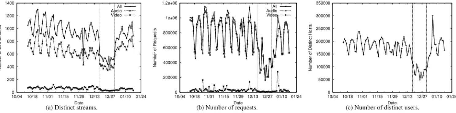
The logs were collected over a 3-month period from October 2003 to January 2004. The daily statistics for live streaming traffic during that period are depicted in Figure 1. The traffic consists of three of the most popular streaming media formats, Apple Quick-Time, Microsoft Windows Media, and Real. As Figure 1(a) shows, there were typically 900-1,000 distinct streams on most days. How-ever, there was a sharp drop in early December and a drop again in mid-December to January (denoted by the vertical lines). This is because we had a problem with our log collection infrastructure and did not collect logs for one of formats on those days. Figure 1(b) depicts the number of requests for live streams, which varies from 600,000 on weekends to 1 million on weekdays. Again, the drop in requests from mid-December onwards is due to the missing logs. The total number of distinct client IP addresses served is roughly 175,000 per day, as depicted in Figure 1(c). The patterns mimic the total number of requests. On average a distinct IP address issues 4 requests.

2.5 Audio vs. Video Event Identification

The logs do not specify content type information. In order to identify whether a stream corresponds to an audio or video stream, we look at the encoding bit rate. The encoding rate is estimated from the logs using the median of the receiving bandwidth that clients report back to the server across all clients receiving the same stream. We use the median (as opposed to the mean) as it is more robust to large errors which may bias the estimate. Figure 2(a) de-picts the cumulative distribution of received bandwidth for an audio stream. Note that most hosts are receiving at 20 kbps, and the me-dian is at 20 kbps. The mean, however, is at 27 kbps because there were a few log entries that erroneously reported bandwidth values of up to Mbps, biasing the mean.

Figure 2(b) depicts the cumulative distribution of estimated en-coding rate for all streams across the 3-month period. A stream is

(3)

0 200 400 600 800 1000 1200 1400 10/04 10/18 11/01 11/15 11/29 12/13 12/27 01/10 01/24

Number of Live Streams

Date

All Audio Video

(a) Distinct streams.

0 200000 400000 600000 800000 1e+06 1.2e+06 10/04 10/18 11/01 11/15 11/29 12/13 12/27 01/10 01/24 Number of Requests Date All Audio Video (b) Number of requests. 0 50000 100000 150000 200000 250000 300000 350000 10/04 10/18 11/01 11/15 11/29 12/13 12/27 01/10 01/24

Number of Distinct Hosts

Date

(c) Number of distinct users.

Figure 1: Daily summary of all live streams from October 2003 - January 2004.

0 0.1 0.2 0.3 0.4 0.5 0.6 0.7 0.8 0.9 1 0 50 100 150 200 250 300 350 400 450 500

Cumulative Probability Distribution

Bandwidth (kbps) mean 27.32, samples 47638

(a) CDF of received bandwidth for one stream.

0 0.1 0.2 0.3 0.4 0.5 0.6 0.7 0.8 0.9 1 0 50 100 150 200 250 300 350 400 450 500

Cumulative Percentage of Streams

Stream Bit Rate (kbps)

(b) CDF of estimated encoding rate for all streams.

Figure 2: Encoding bit rate.

Data Segment Number of Streams Number of Requests

All 88,469 (100%) 73,702,974 (100%)

DailyTop40 9,068 (10%) 49,615,887 (67%)

Large 660 (1%) 23,452,017 (32%)

Table 1: Number of streams and requests in each data set.

classified as video if its encoding bit rate is more than 80 kbps. Note that roughly 22% of streams could not be classified because there are not enough useful data points to estimate the encoding rate. This happens often for streams where there are very few clients, and none of the clients have a bandwidth field in their log entries. Roughly 71% of all streams are audio, most of which use a 20kbps encoding rate. Only 7% are video, using a wide range of encoding rates from 100-350 kbps.

Going back to the daily summary statistics presented in Fig-ure 1, 600-800 of the daily streams are audio, and only 50 of the daily streams are video. Most of the requests are for audio streams, and roughly 50,000 of the daily requests, less than 1%, are for video streams.

2.6 Data Sets

For the analysis in the following sections, we split the data into the three sets listed in Table 1. The setAllis the data for the entire 3-month period. The setDailyTop40is composed of the top 20 most popular audio and top 20 video streams for each of the three encoding formats for every day in the 3-month period, a total of 9,068 streams. The setLargehas all the large-scale streams with peak stream sizes of more than 1,000 concurrent clients. There are a total of 660 large streams. As it happens, these streams are a subset of theDailyTop40set. The remaining 8,408 streams in the

DailyTop40have smaller peak sizes.

To our knowledge, our data set is the most extensive live

stream-ing data in terms of number of streams and requests studied to date. The streams served by Akamai are samples of the type of content currently streamed on the Internet. We acknowledge that our data set may not be a representative sample, as the data is likely biased towards large and popular content publishers who are customers of Akamai. For example, the folklore from ISP operators is that adult content is a popular type of streaming content. However, Akamai serves little to none adult content.

2.7 Macroscopic Analysis

Given the amount of data we have, it is infeasible to analyze and present each stream in detail. Rather, our methodology is to selectrepresentative statisticsfrom each stream, and present the distribution of those statistics across all streams. When we wish to illustrate a finer point, we look at smaller data sets or individual streams.

3. POPULARITY OF EVENTS

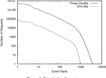
To understand how requests are distributed amongst the events, we look at the popularity of events, as depicted in Figure 3. Popu-larity, here, is defined as the total number of requests for each event across the entire 3-month period as shown on the y-axis. The x-axis is the rank of the stream. Both axes are in log-scale. We find that the popularity distribution is Zipf-like with 2 distinct modes.

Flatter: For 1,000 of the most popular streams with 10,000-7.3 million requests, the popularity distribution fits a straight line, exhibiting Zipf behavior, with an of 1.01.

Steeper: For the remaining streams, which are less popular, with fewer than 10,000 requests the popularity is Zipf-like, but with an much larger than 1. We hypothesize that this

(4)

un-1 10 100 1000 10000 100000 1e+06 1e+07 1 10 100 1000 10000 Number of Requests Event Rank Three months One day

Figure 3: Popularity of events.

likely to pay a CDN to host unpopular content, as a single server hosted by the content publisher may suffice to get the job done.

To see what the popularity distribution looks like at smaller timescales, we randomly pick one day from our logs, and plot the popularity distribution of requests that arrived on that one day on the same scale as the 3-month distribution. As depicted in Figure 3, the one-day distribution looks similar to the 3-month one.

Our findings are in contrast to previously studied popularity dis-tributions for Web objects that report that the popularity is Zipf-like with only one mode [11, 9, 15, 2, 5]. However, a 2-mode Zipf distri-bution is consistent with studies of on-demand streaming objects [1, 6] and multimedia file-sharing workloads [12].

4. CLASSIFICATION OF STREAMS

In this section, we present a scheme for classifying streams (24-hour chunks of events) into types. We use this classification throughout the paper when we wish to show that certain properties are related to the type of stream.

4.1 Large vs. Small

There are several definitions oflargestreams: total number of requests (discussed in Section 3), total unique clients, and peak con-current clients. While all three definitions are related, for this paper, we choose the third definition: peak concurrent clients as it is an indicator of how much server capacity needs to be provisioned to accommodate the stream. Using the definition from Section 2, large streams have a peak of at least 1,000 concurrent clients. Out of our 3-month data set, 660 streams are large. All other streams aresmall.

4.2 Non-Stop vs. Short Durations

Non-stop streamsare streams that are broadcast live every day, all hours of the day. This is similar to always being “on-the-air” in radio terminology. On the other hand,short duration streamshave well-defined durations typically on the order of a few hours. An example of a short-duration stream is a talk show that runs from 9am-10am that is broadcast only during that period, and has no traf-fic at any other time during the day. To distinguish between these two stream types we look at the stream duration. However, the logs do not provide us with any explicit stream duration field. Therefore, we estimate the stream duration using two different methods. We then compare the resulting classification to confirm the accuracy of the methods.

The first method follows directly from our definition that a non-stop stream is always on 24-hours a day. To capture that prop-erty, we estimate the “stream duration” from the logs. We define the stream duration as the period of time for which the stream has or more concurrent receivers, where is set at 10. A threshold of 10 is relatively robust at estimating stream duration for large streams. If a stream duration is roughly 24 hours, then it is a non-stop stream.

Note that this methodology does not work for small streams. For example, consider an unpopular non-stop radio station that has a sparse audience of 1-2 concurrent clients during the day and no clients at night even though the content is available 24 hours a day. Even with an

of 1, we would estimate the stream duration to be only during the day, which is incorrect. For correctness, we only classify large streams.

The cumulative distribution of stream durations for large streams is depicted in Figure 4(a). The x-axis is the stream duration, and the y-axis is the CDF. We find that 76% of streams are non-stop, and the remaining 24% have short durations. We also experimented with other

values and did not find significant differences except for when the threshold was very low (1 or 2). In such cases, this method was susceptible to including “idle time” in the stream du-ration when one or two clients access the URL for a short dudu-ration stream before the stream officially started.

The second method examines the slope of the tail of the ses-sion duration distribution, where a sesses-sion duration is defined as the amount of time a request lasts (how long the client associated with the request receives data). If a stream’s tail has a steep slope, it is a short duration stream. See Section 5.2 for a more detailed descrip-tion of this property. Figure 4(b) depicts the cumulative percentage of streams and the slope of the tail. Roughly 20% of streams had a tail slope of -4 or steeper (where steeper means a more negative number).

We then compared the streams classified using the two meth-ods against one another and found a good agreement: roughly 92% matched. When the two methods did not agree, it was for streams that were short, but had relatively long stream durations (close to 24 hours).

We wish to note that in our data set, all video streams were short. It is possible that the higher cost of delivering non-stop video compared to audio is a deterrent for content publishers.

4.3 Recurring vs. One-Time

A recurring stream is defined as one in which the event URL (say Radio Station X) shows up on multiple days. Recurrence may be periodic, for example, a daily event. Or, it may follow a pre-determined schedule, for example, a cricket series will often use the same URL for many of its matches throughout the series. We find that 97% oflargestreams are recurring. Note that all non-stop streams are recurring by definition. However, there are also recurring short duration streams, such as daily 2-hour talk shows. About 21% of large streams are these short recurring streams.

4.4 Flash Crowd vs. Smooth Arrivals

During a flash crowd, there is a large increase in the number of people wanting to tune in to the stream. In turn, the arrival rate and total number of concurrent clients increase at a rate that is higher than average. A stream with smooth arrivals, on the other hand, sees either no change or gradual changes (due to time of day effects).

All short durationstreams have flash crowd behavior. Intu-itively, this is because short duration streams take place during a specific period, for example 2 hours. It is natural for people to want to start joining and watching the stream from the beginning. In ad-dition, a number ofnon-stopstreams also have flash crowds. We

(5)

0 0.1 0.2 0.3 0.4 0.5 0.6 0.7 0.8 0.9 1 0 5 10 15 20 25

Stream Duration (hours)

(a) Stream duration.

0 0.1 0.2 0.3 0.4 0.5 0.6 0.7 0.8 0.9 1 -35 -30 -25 -20 -15 -10 -5 0

Tail Slope

(b) Tail slope.

Figure 4: Classify streams as non-stop or short.

believe that there are sometimes specific content-related events that happen for a brief period during the non-stop stream. For example, an invited guest appearance can cause a flash crowd.

To detect whether or not a stream has flash crowd behavior, we look at the stream’s arrival rate over time. We first ran a low-pass filter on the data by looking at “smoothed” arrival rates, averaged over 10-minute windows. Any sudden increase (large slope) in the arrival rate is flagged as flash crowd behavior. We find that setting a minimum threshold at a slope of 3 (a 3-times increase in the arrival rate compared to the previous window) is reasonable based on visual inspection. About 50% of the large streams are detected as having flash crowd behavior.

The prominence of flash crowd events in the streams has several implications on systems design. While there are a few systems de-signs that consider flash crowds [19], the problem has been largely ignored. Our findings indicate that flash crowds are the norm in live streaming workloads and systems must be able to cope with sizable changes in the request volume. The system should be able to support new hosts wanting to connect (in the Akamai network, this requires a DNS-based name resolution to the IP address of a server) and new hosts connecting to the system (a request packet to a streaming server). Over-engineering, redundancy [4], and mecha-nisms for rejecting requests to prevent the system from melt-down in both the DNS and the streaming infrastructure can help. To our knowledge, throughout the 3-month data collection period, the Aka-mai network was able to serve the entire request volume presented to it.

5. SESSION CHARACTERISTICS

In this section, we conduct our analysis on sessions. Recall that a session is defined at the granularity of a client request, i.e., one request is one session. We first look at the session arrival process, and then at the session duration distribution.

5.1 Arrival Process

5.1.1 High-Level Characteristics

Figure 5 depicts the mean and median request interarrival times for the DailyTop40 streams from all days, separated into large streams vs. the small streams in the DailyTop40. The first curve on the left depicts the CDF of the observed median interarrival time for all large streams. For example, 70% of large streams had a median interarrival time of 1 second or less. The next curve is the mean interarrival time for large streams, and the next two curves are for the median and mean interarrival times for the remaining smaller streams in the DailyTop40. Note that in interpreting this figure, the

0 0.1 0.2 0.3 0.4 0.5 0.6 0.7 0.8 0.9 1 0.1 1 10 100 1000 10000 100000

Interarrival (seconds)

Large Median Large Mean Small Top40 Median Small Top40 Mean

Figure 5: Mean and median interarrival times for DailyTop40 streams.

order of streams sorted by the median is not necessarily the same as the order sorted by the mean.

We make the following observations. First, the interarrival time is generally shorter for large streams than for smaller streams. The mean time between arrivals is at most 10 seconds for large streams, whereas the mean time can be as high as 10,000 seconds for smaller streams. This makes sense as large streams have more requests. Second, the median interarrival time is generally smaller than the mean indicating that there are some periods where the interarrival time is much longer than the other periods.

In general, the arrival rate varies over time, and the arrival pro-cess is not stationary over large timescales. We analyze the arrival process at shorter (stationary) timescales and find that exponen-tial distributions can be used to model request interarrivals. Our findings are consistent with previously studied arrival processes of on-demand streaming servers [1], live streaming servers [23], and MBone multicast groups [3]. We do not present the modeling re-sults due to space limitations.

Next, we discuss two types of behavior that contribute to changes in the arrival rate: time-of-day effects and flash crowds.

5.1.2 Time-of-Day Behavior

To illustrate that the arrival rate does indeed vary over time, we show the number of active clients tuning in to anon-stopradio station over a one-week period in Figure 6(a). The x-axis is the date, and the y-axis is the number of clients. There are 7 peaks, corresponding to the peaks on each day of the week. The smaller

(6)

0 200 400 600 800 1000 1200 10/14 10/15 10/16 10/17 10/18 10/19 10/20 10/21 Number of Hosts Date All UK US PL

(a) Group membership.

0 5 10 15 20 25 30 35 40 14 15 16 17 18 19 20 21

Arrival Rate (clients/minute)

Date

(b) Arrival rate smoothed over 10-minute intervals.

Figure 6: Arrivals for a radio station over a one week period.

peaks correspond to the weekend. The corresponding arrival rates in number of clients/minute are shown in Figure 6(b). Note that the arrivals roughly mirror the weekly and daily trends in the group membership pattern. Over the course of a day, the arrival rates vary from 5 arrivals/minute to up to 20 arrivals/minute.

To better understand the time-of-day behavior, we break the group membership down by country. We map client IP addresses to their geographic location. Figure 6(a) depicts the group member-ship over time for the top 3 participating countries: the UK, the US, and Poland (labelled PL). The daily peaks in the group member-ship are shifted by several hours. The peak for PL occurs roughly 2 hours before the peak in UK. And, the peak in the US follows the UK peak by roughly 4-5 hours. This clearly reflects time-of-day differences as the clients of this one event are scattered across multiple time zones. Interestingly, however, the peaks always occur at around 3-4pm local time. The arrival rates, not shown, are also shifted accordingly. When modeling arrival processes, one must also consider different arrival rates for clients from different time zones.

5.1.3 Flash Crowds

This particular stream is interesting in that in addition to the weekly and daily cyclical trends, there is also some flash crowd behavior where the arrivals peak as high as 40 arrivals/minute com-pared to the usual 20 arrivals/minute. Flash crowds occurred on 3 separate days, on the 15th, 16th and 17th. US clients caused the flash crowds on the 15th and 17th, whereas UK clients caused a smaller flash crowd on the 16th.

Our observations for this particular radio station holds for many other non-stop streams. For short duration streams, we see less time-of-day and time-zone related behavior, as client requests are perhaps driven by the content itself. Perhaps people are willing to tune in to a short duration stream at 4am in the morning if the con-tent is meaningful to them. One interesting observation is that all

0 0.1 0.2 0.3 0.4 0.5 0.6 0.7 0.8 0.9 1 0.01 0.1 1 10 100 1000 10000

Session Duration (minutes) Large Median

Large Mean Small Top40 Median Small Top40 Mean

Figure 7: Mean and median session duration for DailyTop40 streams.

short duration streams exhibit flash crowd behavior, and some non-stop streams such as the one in Figure 6 also exhibit flash crowd behavior on some days. Overall, we find that 50% of large streams have flash crowds as reported in Section 4.4.

5.2 Session Duration

5.2.1 High-Level Characteristics

Figure 7 depicts the mean and median session duration times in minutes for all the DailyTop40 streams from all days, separated into large streams vs. the remaining smaller streams in the DailyTop40. The first two curves on the right correspond to the mean and median session durations for large streams, whereas the two curves on the left correspond to the remaining smaller streams.

As one would expect, large streams have much larger session durations than smaller streams. In terms of statistical measures of correlation, we find that the correlation coefficient between a group’s peak size and its median session duration is small at 0.2, but the Spearman’s rank correlation is much stronger at 0.7. Rank correlation gives a picture of how the rank of the streams sorted by peak group size agrees with the rank sorted by median session duration.

We make two additional observations from Figure 7. First, for a small portion of the streams, the median session duration is ex-tremely small–less than 10 seconds. While we do not know the actual cause of such small session durations, we hypothesize that some of it may be caused by “channel surfing.” Such small val-ues can have implications on systems design. The group member-ship for the stream is changing very rapidly. This indicates that the servers should quickly time-out on per-session state (for example, TCP time-outs should be short such that sockets can be freed for newer connections),and servers should do only a minimal amount of work to set up a session as it will be shut down quickly.

Our second observation is that, for large streams, the session durations are heavy tailed as the observed mean is much larger than the median for all sessions. There are a few clients who tune in to the content for very long periods, whereas most clients only stay for much shorter periods. The first curve from the right depicts the CDF of the observed mean session duration for all large streams. For example, all large streams had a mean session duration larger than 30 minutes, and almost all (99.7%) had a mean session duration of more than an hour. While the mean is large for most sessions, the median is much shorter, as depicted by the second curve from the

(7)

1e-06 1e-05 0.0001 0.001 0.01 0.1 1 0.01 0.1 1 10 100 1000 10000 100000

Session Duration (minutes)

(a) Non-stop streams.

1e-06 1e-05 0.0001 0.001 0.01 0.1 1 0.01 0.1 1 10 100 1000 10000 100000

Session Duration (minutes)

(b) Short streams.

Figure 8: Complementary cumulative distribution of session duration for large streams.

right. The median ranges from under 4 minutes to 140 minutes. About 40% of streams had median session durations of shorter than 20 minutes.

5.2.2 Tail Analysis

Next, we focus our session duration analysis on the tail of the distributions for all large streams, where the tail is defined as the last 10% of the distribution. Typically, when modeling session duration distributions, the head and the tail should be modeled using differ-ent distributions. We find that the head of the duration distribution for large streams generally fits a log-normal distribution, which is consistent with previous findings [23]. We did not conduct the tail analysis on smaller streams because there are an insufficient num-ber of data points. For large streams, the total numnum-ber of data points for each stream ranged from 10,000-100,000, which we believe is sufficient for tail analysis.

We use the complementary cumulative distribution (CCDF) to analyze the tail of the distributions. The CCDF is defined as the probability that a value of greater than is observed, or

where is the CDF of a random variable X. Intuitively, a

dis-tribution is heavy-tailed if the CCDF is linear when plot in log-log scale.

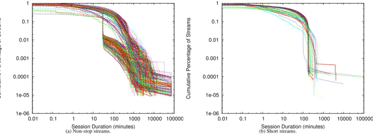
We break up the analysis into non-stop vs. short streams. Fig-ure 8(a) depicts the CCDF for all non-stop streams. Each line rep-resents a stream. The tail is the last 10% of the data in the region below 0.1 on the y-axis and generally falling between 30 and 10,000 minutes on the x-axis. There are 2 distinct shapes for the tail. The group of lines towards the right of the graph have a linear tail, ex-hibiting Pareto heavy-tailed behavior. These correspond to non-stop events that have “always fresh content,” such as radio stations. Ev-ery second, the content is different and newly created. The second set of curves have a characteristic “drop” in the CCDF at around 30 minutes. However, after the 30 minute mark, the rest of the tail looks fairly linear, exhibiting Pareto heavy-tailed behavior. The drop at 30 minutes corresponds to a periodic event. We find that for these streams, the content cycles every 30 minutes. An example is a radio station that plays only headline news. Users do not wish to listen for more than one cycle at a time. We usedaest[7] to estimate the tail and found that for non-stop streams, ranged from 0.7 to 2,

which is consistent with heavy-tailed behavior.

Figure 8(b) depicts the CCDF of the session duration for short events. The common feature is a cut-off point, where the tail abruptly

drops off in the region between 100 and 1,000 minutes on the x-axis. The value at the cut-off point corresponds to the stream duration (for example, there were many streams whose cut-off points were at approximately 3 hours, for a 3-hour talk show). Note that this feature is present irrespective of whether or not the content is audio or video. One interesting observation is that even with the cut-off point, the session duration distribution has a tail. The data can be modeled by using a “truncated” Pareto distribution. To generate data points based on the model, we first estimate the tail parame-ter by extrapolating a line from the curvature of the tail as if there were no abrupt cut-off point. Using the extrapolated tail parameter, we generate a random distribution. Any generated data point with a value larger than the real cut-off point is truncated to the cut-off value. Usingaestto estimate the tail, we found that for all short streams, ranged from 1.13 to 2.

Interestingly, for the 3 different tail behaviors, only one, the non-stop with always fresh content, is caused by user behavior. The other two tails are a result of the nature of the content in that either the content cycles and effective “ends”, or the stream terminates in the case of short events.

5.3 Implications

The combination of session arrival and duration characteristics provide us with group membership dynamics which are useful for evaluating design and architectural choices. For example, we re-cently looked at the influence of the group membership dynamics analyzed in this study on the stability of a peer-to-peer streaming system [22]. In a peer-to-peer system, there is no stable infras-tructure. When a peer leaves the system (i.e., stops watching the stream), some of the other peers in the overlay structure may be-come disconnected and not receive any streaming content. A de-sirable overlay structure is one in which there are minimum disrup-tions. We found that it is feasible to construct stable overlays despite many hosts staying for very short periods. The key insight is that there is a tail–there are a few hosts who stay for very long periods and these hosts can be used to create stability in the overlay struc-ture. Overall, our findings indicate that peer-to-peer architectures can have stability under realistic group membership dynamics.

6. WHAT IS THE TRANSPORT PROTOCOL?

In this section, we look at the transport protocol used to stream content between servers and clients. Generally, UDP is more

(8)

ap-0 20 40 60 80 100 udp tcp unkn own udp tcp udp tcp unkn own rtp http mms rtsp

Quicktime Real Windows media

Pe rc en ta ge o f r eq ue st s

Figure 9: Transport protocol for each media format.

AS domains UDP-dominant TCP-dominant

QuickTime 56% 44%

Real 49% 51%

Windows Media 12% 88%

Countries UDP-dominant TCP-dominant

QuickTime 75% 25%

Real 72% 28%

Windows Media 2% 98%

Table 2: Breakdown of transport protocol usage by AS domain and country.

propriate for streaming because it allows the application to have full control of buffering and retransmission of data. TCP, on the other hand, has strict reliability semantics which may be in conflict with the real-time requirements of live streaming.

Most of the recent versions of the media players, by default, will automatically probe the network to determine the best trans-port protocol to use. Network address translators (NATs), firewalls and ISPs on the path between a client and a server may disallow cer-tain protocols, and probing allows media players to discover which protocols may be used. For example, UDP may not be available for a host behind a firewall that filters UDP. Generally, players prefer UDP over TCP, and will use UDP unless (i) it is not available, or (ii) the user intervenes and configures the player to use TCP. We hypothesize that user intervention is not common.

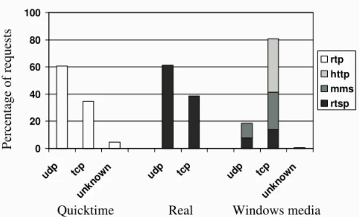
Figure 9 depicts the percentage of sessions seen using each transport protocol. QuickTime and Real have predominantly UDP traffic. However, roughly 40% of sessions are being streamed using TCP. Given that this is consistent across the two formats, we spec-ulate that this may be capturing the state of UDP filtering on the Internet.

To understand whether the use of transport protocols is specific to a region, we break the requests down by AS domains and coun-tries in Table 2. Each region is determined to be TCP-dominant or UDP-dominant based on which protocol was used the most in that region. For QuickTime and Real, roughly 50% of AS domains are TCP-dominant, and over 25% of countries are TCP-dominant.

The transport protocol used by Windows Media, on the other hand, is surprisingly different. TCP sessions are clearly the major-ity, at 80% of all sessions, with HTTP dominating the other stream-ing protocols. Microsoft’s proprietary streamstream-ing protocol, MMS, is the second most used. To understand why there are much more TCP sessions compared to the other streaming formats, we look carefully at how the player probes the network. Version 9 of the Windows Media Player uses the following prioritization by default: (i) RTSP/TCP, (ii) RTSP/UDP, and (iii) HTTP, with MMS only used

0.00E+00 2.00E+05 4.00E+05 6.00E+05 8.00E+05 1.00E+06 1.20E+06 1.40E+06 1.60E+06 US_CN DE ES FR GB CA JP PT CH BE MX NL SE KR BR AU PL IR IT Countries N um be r o f I P A dd re ss es

Figure 10: Geographic clusters across all DailyTop40 streams.

as the last resort. Note that older players will strictly prioritize UDP over TCP. However, our data shows that HTTP, not RTSP/TCP is the dominant protocol. Looking further, perhaps our measurements for Windows Media are capturing an Akamai-specific server con-figuration that prioritizes HTTP connections. The reason for us-ing HTTP is that it has been shown that HTTP scales better than the other streaming protocols for the Windows Media Server [18]. Therefore, the numbers from Windows Media may not necessarily be representative of transport protocol use on the Internet.

To summarize, we find that roughly 40-50% of the AS domains are TCP-dominant. We hypothesize that hosts from such domains are behind NATs or firewalls that limit the range of UDP commu-nications. This has implications on the deployment of UDP-based congestion control protocols [10]. Deployment may be limited to domains that allow UDP, and universal communications using UDP may not be possible. In addition, our findings have similar impli-cations on the deployment of new appliimpli-cations and services in the network, as they may need to be restricted to using TCP.

7. WHERE ARE HOSTS FROM?

In this section, we look at the distribution of clients tuning in to live streaming media.

We answer the following questions:

Where are clients from?

What is the coverage of a stream?

What is the relative distance between clients participating in the same stream?

7.1 High-Level Characteristics

Figure 10 indicates where the clients of the DailyTop40 streams are from. The x-axis is countries. The y-axis is the number of IP ad-dresses from each country. The mapping from IP address to country is obtained using the methodology described in Section 7.2. Over-all, there are IP addresses from 223 countries in the trace, but for presentation purposes we only show the 20 most common countries in this figure. The country with the largest number of IP addresses is the US, which has twice as many IP addresses as any of the next 4 countries: China, Germany, Spain, and France. The participation from all of Europe dominates all other continents.

7.2 Granularity of Locations

We look at locations at four different granularities: AS do-mains, cities, countries, and time zones. AS domains represent

(9)

network-level proximity. Geo-political regions of cities and coun-tries provide us with insight into the diversity (or lack thereof) of people who are tuning in to streams. This also provides us with in-sight into whether or not Internet streaming is enabling new modes of communications reaching wider audiences than traditional radio or local TV stations which have physically concentrated audiences (within a few towns or cities). In addition, we would like to know how well the Internet’s truly “global” reach, crossing countries and oceans, is currently being exploited. Time zones provide insight on the relative distance between people. Perhaps people in the same time zone are likely to have similar behavior compared to people from different time zones due to time-of-day effects.

To map an IP address to a location, we use Akamai’s EdgeScape tool, a commercial product that maps IP addresses to AS domains, cities, countries, latitude-longitude positions, and many other geo-graphic and network properties. The mapping algorithms are based on many sources of information, some of which are host-names, traceroute results, latency measurements, and registry information. We have compared the EdgeScape IP-to-AS mapping with the map-ping extracted from BGP routing tables available from the Route Views project [20], and have found that the mappings are a near perfect match. We also verified the country-level mapping, using the freely available GeoIP database [17], and found the differences between the EdgeScape and GeoIP to be negligible. We manu-ally verified the city-level mapping for some DSL IP addresses and university campuses (our own and others) and found it to be accu-rate. More formal verification [16] showed that the mapping results from EdgeScape are consistent with results from another commer-cial mapping tool, Ixia’s IxMapper [13].

We note that EdgeScape does not provide us with time zone information. We estimate the time zone by bucketing longitudes into 15 degree increments, roughly corresponding to time zones.

7.3 Metrics

Next, we zoom in to each stream to better understand how clients are distributed. We look at three metrics that capture client diversity, clustering, and the distance between clients.

Diversity Index

Our first metric, thediversity indexis defined as the number of distinct “locations” (AS domains, cities, countries, or time-zones) that a particular stream reaches. For example, if a stream is viewed by only clients located in the United States, the country diversity index is a low value of 1.

Clustering Index

Theclustering index, our second metric captures how clustered or skewed the client population is, and is defined as the minimum number of distinct locations that account for 90% of the IP ad-dresses tuning in to each stream. For example, if 95% of clients are located in the United States, 3% are in the UK, and 2% are in Poland, the clustering index is 1. If the clustering index is small, then only a small number of locations account for most of interests in the streams.

Radius Index

The above two metrics give us a count on the number of distinct locations, but does not provide us a proximity measure of how these locations relate to one another. For example, if a stream covers 2 distinct time zones, are these time zones next to each other on the same continent, or is one of them on one continent and the other one on another continent halfway around the world? To capture the distance between locations, we use the time zoneradius index

which captures the spacing between client time zones.

To compute the radius index for each stream, we compute the centroid time zone defined as the time zone in which the average distance between the centroid and all points (all time zones weighted

0 0.1 0.2 0.3 0.4 0.5 0.6 0.7 0.8 0.9 0 2 4 6 8 10 12 Percentage of IP Addresses

Distance (Number of Time Zones)

Figure 11: Percentage of IP addresses at each distance from centroid time zone.

by the number of clients in each time zone) is minimized. For ex-ample, for a stream in which there are people from two time zones, half from the US East coast and the other half in the UK, the cen-troid time zone would be somewhere in the middle in the Atlantic Ocean. We then compute the distribution of clients as a function of how far away they are from the centroid. Figure 11 depicts this distribution for all large streams in the trace, each line representing a stream. Note that for some streams, most of the mass is at 0 ra-dius, meaning that most clients are in the same time zone. For a few other streams, the peak is at 1, meaning most hosts are one time zone away from the centroid. A peak at 6 means that most hosts are 6 time zones away from the centroid. Location-wise, this means that there are two large bodies of mass half-way around the world (12 time zones) from each other. As a representative statistic, the radius index is the minimum distance (radius) at which 90% of all clients are covered. A small radius index means that most of the population are “close” to each other, whereas a large index means the population are “far” apart.

7.4 Large vs. Small Streams

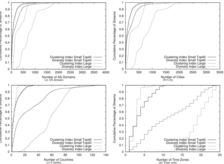
Figure 12 depicts the diversity and clustering index for all Dai-lyTop40 streams, separated into large vs. small streams. The indices for AS domain and city granularities are shown in Figures 12(a) and (b). Note that the two granularities look very similar. Perhaps this reflects that there are a large number of small or regional AS do-mains, and/or, that the EdgeScape mapping of IP address to city may assign all IP addresses that belong to an AS to the same city if it does not have any better information in its database. We wish to make two observations. First, for large streams, the diversity of AS domains (the right-most curve) is wide, ranging from 200-3,500 distinct domains. At the city-level, the diversity is also from 200-3,500 cities. This range is much larger than traditional radio and TV broadcasts that are physically limited to a few towns or cities. The clustering index for large streams (second line from the right) is also relatively large–again, reflecting the wide coverage. Roughly 90% of IP addresses are from 10-1,000 cities/AS domains. Second, the diversity and clustering indices for smaller streams (the two lines on the left) are generally smaller than large streams. However, the index is still large in that half of the small streams cover 100 cities or more! This reflects the power of the Internet as a transmission medium as it does not share the same physical limitations on its transmission range as traditional local radio or TV.

(10)

0 0.1 0.2 0.3 0.4 0.5 0.6 0.7 0.8 0.9 1 0 500 1000 1500 2000 2500 3000 3500 4000

Number of AS Domains

Clustering Index Small Top40 Diversity Index Small Top40 Clustering Index Large Diversity Index Large

(a) AS domain. 0 0.1 0.2 0.3 0.4 0.5 0.6 0.7 0.8 0.9 1 0 500 1000 1500 2000 2500 3000 3500

Number of Cities

(b) City. 0 0.1 0.2 0.3 0.4 0.5 0.6 0.7 0.8 0.9 1 0 20 40 60 80 100 120 140

Number of Countries

(c) Country. 0 0.1 0.2 0.3 0.4 0.5 0.6 0.7 0.8 0.9 1 0 5 10 15 20 25

Number of Time Zones

(d) Time zone.

Figure 12: Diversity and clustering index for DailyTop40 streams: large vs. small.

Figure 12(c). The right-most line is the diversity index for large streams, and the second line from the right is the diversity index for small streams. Again, large streams generally have more diversity. However, it is surprising that even small streams can have diversity, as well. For example, 50% of small streams cover 10 countries or more. Next, we look at the clustering index. Large streams have very skewed clustering, as almost all large streams have a cluster index of 10 countries or less. However, for 15% of small streams, the clustering index is larger than 10 countries, indicating that these small streams are more geographically “scattered.”

Figure 12(d) depicts the time zone diversity index. Note that almost all large streams reach more than half of the world (13 or more time zones). However, small streams reach a number of time zones, uniformly distributed across the entire range. The time zone clustering index has similar behavior to the country clustering in-dex. For over 90% of large streams, the clustering index is 4 time zones, whereas for 90% of small streams, the clustering index spans 8 time zones.

To understand the spacing and the distance between clients’ time zones, we look at the radius index depicted in Figure 13. The radius index for small streams ranges from 0 (meaning 90% of clients are in the same time zone) to more than 10 (meaning that clients are uniformly scattered across many time zones). For 50% of the small streams, the radius index is larger than 4, roughly span-ning at anywhere from two continents to the entire world. Around

0 0.1 0.2 0.3 0.4 0.5 0.6 0.7 0.8 0.9 1 0 2 4 6 8 10 12

90th Percentile Radius Index (Number of Time Zones) Large Large Non-stop Large Short Small

Figure 13: Radius index.

65% of large streams have a radius index of 2 or less, indicating that 90% of its clients span just 1 continent.

Next, we ask whether different event types have any impact on the diversity. For our analysis, we classify the set of large streams into non-stop vs. short. We then compute the same indices as dis-cussed in the previous section. We find that short streams are often

(11)

0 0.1 0.2 0.3 0.4 0.5 0.6 0.7 0.8 0.9 1 0 20 40 60 80 100 120 140

Number of Countries

(a) Country. 0 0.1 0.2 0.3 0.4 0.5 0.6 0.7 0.8 0.9 1 0 5 10 15 20 25

Number of Time Zones

(b) Time zone.

Figure 14: Diversity index for simultaneous users.

more diverse and less clustered at the granularity of AS domains and cities. However, at larger location granularities of countries and time zones, non-stop streams tend to be more diverse. The cluster-ing properties for countries and time zones are similar, regardless of event types. Due to space constraints, we omit the figures from the paper.

The radius distance depicted in Figure 13 for non-stop vs. short streams are not that different. However short streams tend to have a larger radius index, covering more of the world.

7.5 Simultaneous Users

In the previous section, we analyzed the properties of clients across 24-hour-long streams. The findings reflect the total clients who request the stream across the entire 24-hour period. In this section, we zoom in to finer timescales. We divide the streams fur-ther into 1-hour chunks and run the same analysis across all 1-hour chunks. This approximates clients who are accessing a stream “si-multaneously.” If time-of-day effects are common, we expect to see less diversity at smaller timescales.

Figure 14 depicts the diversity and clustering indices for coun-try and time zone granularity. First, we note that compared to Fig-ure 12(c), the country diversity index in FigFig-ure 14(a) is shifted to-wards the left, indicating less diversity at smaller timescales. Sec-ond, however, the clustering indices are only slightly different indi-cating that the a few countries tend to dominate and the clustering properties hold at different timescales.

The time zone diversity is also less at smaller timescales as de-picted in Figure 14(b). The time zone clustering remains similar compared to Figure 12(d). While time-of-day effects have signif-icant influence on the diversity index, it has little influence on the clustering of hosts.

7.6 Implications

We find that many of the streams are diverse at multiple gran-ularities. The most interesting finding is that there is a wide range of diversity even for small sized streams. The high degree of diver-sity has many implications on designing content distribution sys-tems. One example is how should a content distribution system be designed so that it can provide global reach, and at the same time scale to the number of clients and the channels. Clearly, how to place servers at the right locations in the network to reach 10,000 simultaneous users across 2,000 AS domains for one channel is a challenge in its own right. Adding more channels, large and small,

all wanting global reach, increases the level of difficulty of the prob-lem. To add another dimension, to achieve load balancing, efficient use of resources, and good performance in the face of changing dis-tributions of clients, a dynamic mapping of clients to servers may be required.

8. CLIENT BIRTH RATE AND LIFETIME

In this section, we look at client participation and retention. We ask two questions:

Are new clients tuning in to an event?

What is the lifetime of a client?

8.1 Methodology

The data we use for this analysis is drawn from the DailyTop40 set. Our analysis is conducted on the granularity of events. We use only data for events that are recurring, where recurring means that the event took place at least twice across the 3-month period. Examples of recurring events are 24-hours a day, 7-days a week radio stations, regular daily talk shows, and sports events that take place a few times a month.

To identify distinct users, we use the player ID field in the logs. Note that this field is available only for the Windows Media for-mat. The other two formats do not appear to support this feature as the field is either blanked or all zeros in the logs. For Windows Media, the ID is unique unless the player has been configured for anonymity. Anonymized IDs have a well-specified prefix, and are removed from the analysis. This eliminates half of the requests from our traces. We assume that participation behavior is independent of whether or not a user configures his/her browser for anonymity. While our analysis is conducted for only one of the streaming for-mats, we have conducted analysis using client IP addresses (as op-posed to player IDs) to identify unique users for the other formats. The results appear to have similar trends. However, we do not report them in this paper because there are several weaknesses to using IP addresses as a unique identifier: (i) the presence of NATs, firewalls, proxies, and DHCP could mistakenly identify multiple clients as one user (sharing one IP address), and (ii) the use of DHCP could mistakenly identify one client as multiple users (when assigned to different IP addresses).

(12)

0 10 20 30 40 50 60 70 80 90 100 0 0.1 0.2 0.3 0.4 0.5 0.6 0.7 0.8 0.9 1

Cumulative Percentage of Events

Birth Rate

All Recurring Large Recurring Large Non-Stop Large Short

(a) Birth rate by type.

0 0.1 0.2 0.3 0.4 0.5 0.6 0.7 0.8 0.9 1 10/04 10/18 11/01 11/15 11/29 12/13 12/27 01/10 01/24 Birth Rate Date Non-stop Short (b) Birth rate. 0 1000 2000 3000 4000 5000 6000 7000 8000 9000 10/04 10/18 11/01 11/15 11/29 12/13 12/27 01/10 01/24

Number of Distinct Users

Date

Non-stop Short

(c) Distinct users.

Figure 15: Birth rate for recurring events.

8.2 New Client Birth Rate

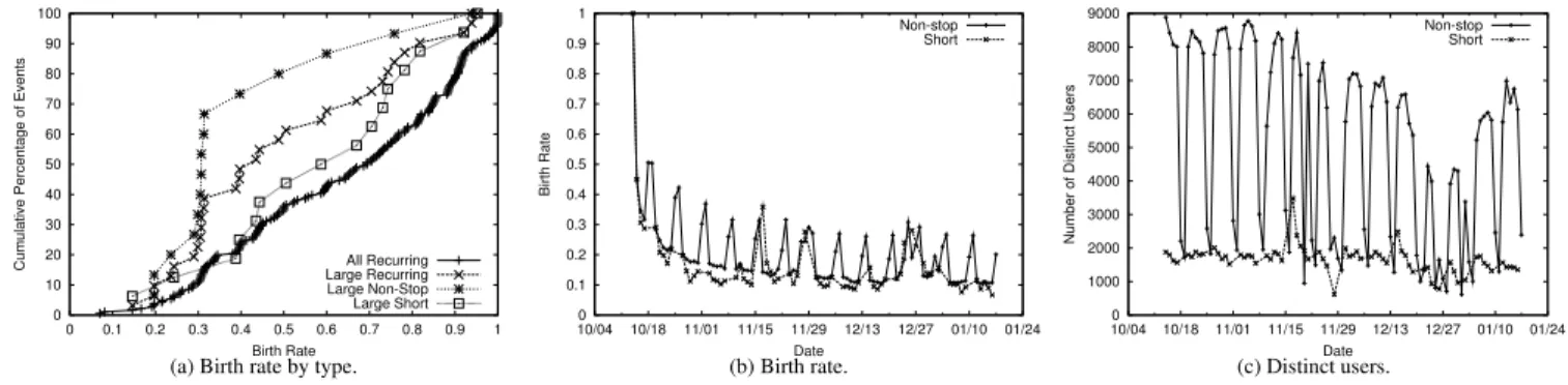
To understand whether new clients are tuning into the system, we look at clientbirth rate, where the birth rate is defined as the ratio between the number of new distinct users that showed up that day over the number of total distinct users for that day. Note that new is determined relative to all the previous days in the data set. For example, on the first day, all users are newly born and the birth rate is 100%. On the third day, only users who did not show up on the first and second day are counted as new. Figure 15(a) depicts the average birth rate, excluding the first day, for all DailyTop40 recurring events. The x-axis in the figure is the average birth rate. The y-axis is the cumulative distribution of events. Note again that an event means the aggregate of all streams that belong to the same URL across multiple days. The birthrate varies from 10% to 100%, and all values of birthrates are uniformly observed across the entire set of events.

Next, we look at the distribution for events that contained large streams, also depicted in Figure 15(a) and find that it is also spread across all birth rates, but with lower birth rate values compared to all DailyTop40 recurring events. Further, we break the events with large streams into non-stop (the line at the top) vs. short. We find that the birth rate for non-stop events is more concave and much lower compared to short events. To understand what causes a higher birth rate for short events, we looked at the frequency with which short events recur. We find that short events that occur back-to-back (almost every day) have much lower birth rates than events that occur only a few times sparsely spread over the 3-month data collection period. This indicates that more users are retained when streaming events occur closer to each other.

Figure 15(b) depicts the birth rate for two recurring events with large streams, a US-based non-stop radio station and a US-based short duration event (3-hour talk show). The y-axis is the birth rate, and each point on the x-axis corresponds to a day. Roughly 10-30% of users are newly born every day. For the US-based radio station, a distinct pattern in the birth rate emerges, where the birth rate alternates between a low value during the weekday (valley), and a much higher value during the weekend (peak).

However, in terms of the total number of distinct users depicted in Figure 15(c), there were 2-4 times more users on weekdays than weekends. How can the birth rate be so much higher? Perhaps this is because during the weekend, people are tuning in using their home computers, which have different player IDs than the one on their computer at work. In addition, the rate is much higher be-cause it corresponds to all the new people who tuned in during the weekday, and are tuning in from home during the weekend.

The birth rate for the short event program is roughly 10%. Note that there are no weekend/weekday patterns because the content is only available on weekdays. There are a couple of days with peaks.

This first one is on Nov 17, which corresponds to a 2-fold increase in the number of distinct users in Figure 15(c). Another set of peaks happens around Dec 23-26 (Christmas holiday). Note that in this case, the number of distinct users is much less than usual. Perhaps the spike in birth rates are caused by people using their home com-puters or their relatives’ comcom-puters to tune in during the holiday.

8.3 Client Lifetime

Overall, the number of distinct users for the short event remains approximately constant except for a few days where there are peaks, and a slight decrease over the holiday season. The number of dis-tinct users for the non-stop event has weekly trends, but is roughly constant across all weekdays and constant across all weekends with some similar seasonal behavior during the holidays. Given that the birth rate is 10%, this means that the events are losing viewers at roughly 10% as well.

Next, we ask, who is leaving: the new-comers, or the old-timers? To answer this, we look at the lifetime of clients tuning in to the two events as depicted in Figure 16(a). For both events, nearly half of all users, which we callone-timers, only stay for one day. This indicates that most new-comers have short lifetimes and the system has steady participation because of the old-timers.

To understand the overall role of new-comers and old-timers, we run an analysis across all recurring events. In our analysis, we look at the averagelifetimeof clients for each event, where lifetime is defined as the number of days from when the client first showed up to when the client was last seen tuning in to the event. The def-inition is biased towards short lifetimes for people who were born later in the data set. To account for such biases, we only conduct the analysis for clients who were born in the first half of the data set.

Figure 16(b) plots the cumulative distribution of the number of one-timers for all recurring events. For roughly 90% of the events, more than 50% of the users are timers. The number of one-timers is surprisingly high. We believe that there are several causes for this. First, this captures user behavior when users are “checking out” the event to see whether or not they like it. If they do not like it, they never come back. Second, the percentage of one-timers is correlated with the frequency at which the event recurs. For exam-ple, we compared a radio station that is recurring on a daily basis to a sports event that happens twice a month and found that the radio station has a lower percentage of one-timers.

Next, we look at the average lifetime of clients that are not one-timers. Figure 16(c) plots the average lifetime of users for each of the events. The x-axis is the average lifetime in days, and the y-axis is the event duration in days. Points that fall on the line ( ) means that all users have an average lifetime that is equal to

the event duration. For many events that recur daily, the average lifetime of clients can be up to 60 days. Overall, for most events, if

(13)

0 0.1 0.2 0.3 0.4 0.5 0.6 0.7 0.8 0.9 1 0 10 20 30 40 50 60 70 80 90 100

Cumulative Percentage of Users

Life Time (Days) Non-stop

Short

(a) Lifetime for two recurring events.

0 0.1 0.2 0.3 0.4 0.5 0.6 0.7 0.8 0.9 1 0.1 0.2 0.3 0.4 0.5 0.6 0.7 0.8 0.9 1

Cumulative Percentage of Events

Percentage of One-Timers

(b) Percentage of one-timers in each event.

0 10 20 30 40 50 60 70 80 90 100 0 10 20 30 40 50 60 70

Event Duration (Days)

Life Time (Days)

(c) Average client lifetime excluding one-timers.

Figure 16: Client lifetime.

a client shows up more than once, it will have an average lifetime of at least one-third of the days in the event.

8.4 Implications

To summarize, we have shown that for all events the birth rate for new clients tuning in is roughly 10% or more. Roughly 50% or more new clients are one-timers. However, the events have steady membership because there are enough old-timers that have high av-erage lifetimes. To understand the significance of our findings, we present two examples of design decisions where our observations can be applied. First, the presence of one-timers has direct implica-tions on the scalability of maintaining per-client “persistent” state at servers. Such state may be used by the server to customize content served to clients. To control the amount of overhead in maintaining state, a caching-based algorithm can be used to rapidly time-out on the one-timers, which are at least 50% of the client base. A sec-ond example is that clients can maintain performance history for the servers that it visits. Given that clients keep accessing the same event/server repeatedly over many days, history should be useful for server selection problems.

9. RELATED WORK

Live streaming and MBone workloads

Veloso et al. [23] studied live streaming workloads from a server located in Brazil. The focus of the analysis was on characterizing ar-rival processes and session durations for two non-stop video events to be used in a workload generator. Our findings for arrival pro-cesses and session durations from the Akamai workloads are con-sistent with their findings. However, to contrast, we have also an-alyzed several other properties such as the popularity of streams, the use of transport protocols, the diversity of clients, and the client lifetime.

The join arrival process and session duration distribution for multicast groups on the MBone were also analyzed [3]. The key findings were that interarrivals follow an exponential distribution, and durations fit a Zipf distribution for non-stop multicast groups. For a group with short duration (for example, a 1-hour lecture), the session durations are exponential. While the interarrival find-ings are similar to our workload, the session durations are different. We identified that session durations are heavy-tailed irrespective of whether or not the stream is non-stop vs short duration. However, the shape of the tail is different (Pareto vs. truncated) for different stream types.

Location of users

Faloutsos et al. [8] looked at “spatial clustering” amongst users in (i) Quake I, a network game, and (ii) MBone multicast groups. They focused on AS-level clustering inside a group and correlations amongst groups. They found that for network games, there is

lit-tle clustering. However, there is significant clustering for multicast groups. While we also look at AS-level clustering, we also look at geographical and time-zone clustering. In addition, the number of “members” of streams in our data set is orders of magnitudes larger. AS clustering amongst clients accessing the same web-site has also been studied [14]. The key findings are that cluster sizes are heavily skewed. There are a few very large clusters, and a number of small clusters. In contrast to this study, we are also interested in how these clusters relate to each other in terms of their distance. We look at whether these clusters span the globe, or are concentrated in one geographical location.

Web, on-demand streaming, and peer-to-peer workloads

Many studies of Web workloads have found that the popular-ity of Web objects follows a Zipf distribution [11, 9, 15, 2, 5]. In contrast, we have found that the popularity distribution for live streaming has two modes where the first mode (head) is flatter than the second mode (tail). Studies of on-demand streaming work-loads have also observed a popularity distribution with one [6] or two modes [1]. Session durations often exhibited heavy-tail behav-ior, similar to what we have observed for live streaming. In addi-tion, session interarrivals were found to be approximately exponen-tial during periods of stationary request arrivals. More recently, a bimodal popularity distribution was also observed in peer-to-peer multimedia file-sharing workloads [12].

The join arrival process, session duration distribution, user di-versity, and new host birth rate was analyzed for End System Multi-cast (ESM), a peer-to-peer live streaming system with streams that attract 100-1,000’s of users [21]. Overall the ESM and Akamai live streaming workloads are similar. The join interarrival distribution is exponential and the session duration distribution is log-normal. Similar tail behavior for short duration events were also observed. Despite the small scale deployment, there is a wide diversity in user population with users from more than 15 countries participating in any one stream. Finally, new host birth rate for back-to-back streams was roughly 50% which is high, but slightly lower than the average birth rate of 64% for Akamai streams.

10. SUMMARY

In this paper, we analyzed 3-months of live streaming work-loads from a large content distribution network. We take a macro-scopic approach to identify common trends amongst the various types of content. Specifically, from our data set, we found that:

Most of the live streaming workload today is audio. Only 1% of the requests are for video streams. And only 7% of streams are video streams.

A small number of events, mostly non-stop audio programs like radio, account for a huge fraction of the requests. The popularity distribution is Zipf-like with two distinct modes.