Graph Theory: Penn State Math 485 Lecture Notes. Christopher Griffin

(1)

Graph Theory: Penn State Math 485 Lecture

Notes

Version 1.4.2.1

Christopher Griffin

«

2011-2012

Licensed under aCreative Commons Attribution-Noncommercial-Share Alike 3.0 United States License

With Contributions By: Suraj Shekhar

(2)

(3)

List of Figures

2.1 It is easier for explanation to represent a graph by a diagram in which vertices are represented by points (or squares, circles, triangles etc.) and edges are

represented by lines connecting vertices. 4

2.2 A self-loop is an edge in a graphG that contains exactly one vertex. That is, an edge that is a one element subset of the vertex set. Self-loops are illustrated by

loops at the vertex in question. 5

2.3 The city of K¨onigsburg is built on a river and consists of four islands, which can be reached by means of seven bridges. The question Euler was interested in answering is: Is it possible to go from island to island traversing each bridge only once? (Picture courtesy of Wikipedia and Wikimedia Commons: http://en.wikipedia.org/wiki/File:Konigsberg_bridges.png) 5 2.4 Representing each island as a dot and each bridge as a line or curve connecting

the dots simplifies the visual representation of the seven K¨onigsburg Bridges. 5 2.5 During World War II two of the seven original K¨onigsburg bridges were

destroyed. Later two more were made into modern highways (but they are still bridges). Is it now possible to go from island to island traversing each bridge only once? (Picture courtesy of Wikipedia and Wikimedia Commons: http: //en.wikipedia.org/wiki/File:Konigsberg_bridges_presentstatus.png) 6 2.6 A multigraph is a graph in which a pair of nodes can have more than one edge

connecting them. When this occurs, the for a graph G= (V, E), the element E

is a collection or multiset rather than a set. This is because there are duplicate

elements (edges) in the structure. 7

2.7 (a) A directed graph. (b) A directed graph with a self-loop. In a directed graph, edges are directed; that is they are ordered pairs of elements drawn from the vertex set. The ordering of the pair gives the direction of the edge. 8 2.8 The graph above has a degree sequence d= (4,3,2,2,1). These are the degrees

of the vertices in the graph arranged in increasing order. 10

2.9 We construct a new graph G0 from G that has a larger value r (See Expression 2.5) than our original graph Gdid. This contradicts our assumption that G was

chosen to maximize r. 12

2.10 The complete graph, the “Petersen Graph” and the Dodecahedron. All Platonic solids are three-dimensional representations of regular graphs, but not all regular graphs are Platonic solids. These figures were generated with Maple. 14

(6)

2.11 The Petersen Graph is shown (a) with a sub-graph highlighted (b) and that sub-graph displayed on its own (c). A sub-graph of a graph is another graph whose vertices and edges are sub-collections of those of the original graph. 15 2.12 The subgraph (a) is induced by the vertex subset V0 = _{6,7,8,9,10_}. The

subgraph shown in (b) is a spanning sub-graph and is induced by edge subsetE0 =

{{1,6_},_{2,9_},_{3,7_},_{4,10_},_{5,8_},_{6,7_},_{6,10_},_{7,8_},_{8,9_},_{9,10_}}. 16 2.13 A clique is a set of vertices in a graph that induce a complete graph as a

subgraph and so that no larger set of vertices has this property. The graph in

this figure has 3 cliques. 17

2.14 A graph and its complement with cliques in one illustrated and independent sets

in the other illustrated. 17

2.15 A covering is a set of vertices so that ever edge has at least one endpoint inside

the covering set. 18

3.1 A walk (a), cycle (b), Eulerian trail (c) and Hamiltonian path (d) are illustrated. 22

3.2 We illustrate the 6-cycle and 4-path. 23

3.3 The diameter of this graph is 2, the radius is 1. It’s girth is 3 and its

circumference is 4. 24

3.4 We can create a new walk from an existing walk by removing closed sub-walks

from the walk. 25

3.5 We show how to decompose an (Eulerian) tour into an edge disjoint set of cycles,

thus illustrating Theorem 3.26. 26

3.6 A connected graph (a), a disconnected graph (b) and a connected digraph that

is not strongly connected (c). 26

3.7 We illustrate a vertex cut and a cut vertex (a singleton vertex cut) and an edge cut and a cut edge (a singleton edge cut). Cuts are sets of vertices or edges whose removal from a graph creates a new graph with more components than

the original graph. 27

3.8 If e lies on a cycle, then we can repair path w bygoing the long way around the

cycle to reach vn+1 from v1. 28

3.9 Path graph with four vertices. 30

3.10 The graph for which you will compute centralities. 31

3.11 A bipartite graph has two classes of vertices and edges in the graph only exists

between elements of different classes. 32

3.12 Illustration of the main argument in the proof that a graph is bipartite if and

only if all cycles have even length. 33

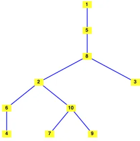
3.13 A tree is shown. Imagining the tree upside down illustrates the tree like nature

of the graph structure. 34

3.14 The Petersen Graph is shown on the left while a spanning tree is shown on the

(7)

3.15 The proof of 4 =_⇒ 5 requires us to assume the existence of two paths in graph

T connecting vertex v to vertex v0. This assumption implies the existence of a

cycle, contradicting our assumptions onT. 37

3.16 We illustrate an Eulerian graph and note that each vertex has even degree. We also show how to decompose this Eulerian graph’s edge set into the union of edge-disjoint cycles, thus illustrating Theorem 3.78. Following the tour construction procedure (starting at Vertex 5), will give the illustrated Eulerian

tour. 40

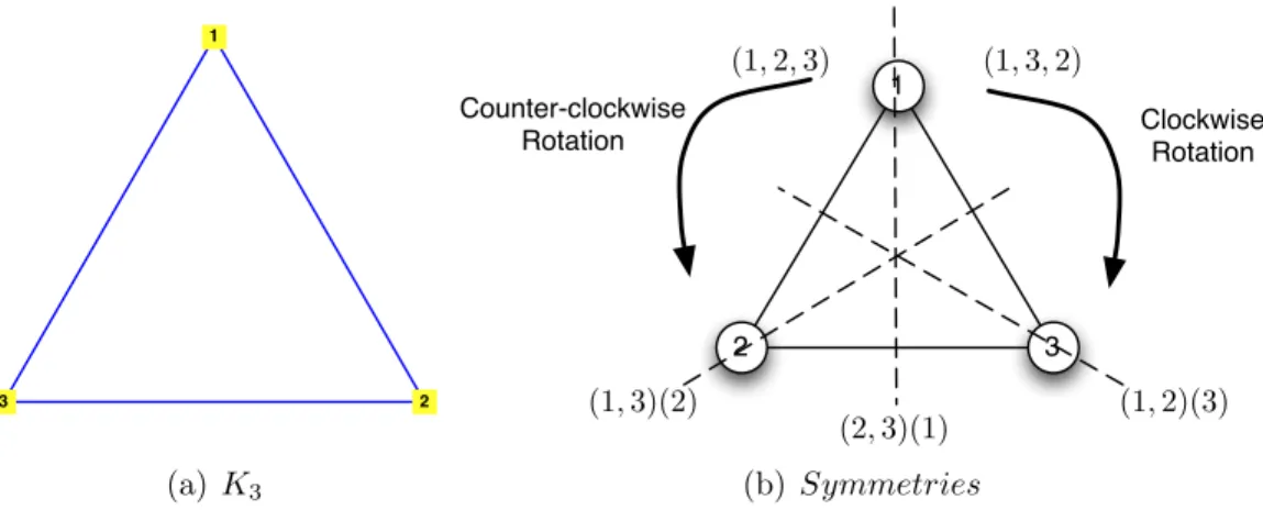
4.1 Two graphs that have identical degree sequences, but are not isomorphic. 42 4.2 The graph K3 has six automorphisms, one for each element in S3 the set

of all permutations on 3 objects. These automorphisms are (i) the identity automorphism that maps all vertices to themselves; (ii) the automorphism that exchanges vertex 1 and 2; (iii) the automorphism that exchanges vertex 1 and 3; (iv) the automorphism that exchanges vertex 2 and 3; (v) the automorphism that sends vertex 1 to 2 and 2 to 3 and 3 to 1; and (vi) the automorphism that

sends vertex 1 to 3 and 3 to 2 and 2 to 1. 46

4.3 The star graphs S3 and S9. 47

4.4 The adjacency matrix of a graph with n vertices is an n_×n matrix with a 1 at element (i, j) if and only if there is an edge connecting vertex i to vertex j;

otherwise element (i, j) is a zero. 50

4.5 Computing the eigenvalues and eigenvectors of a matrix in Matlab can be accomplished with the eig command. This command will return the eigenvalues when used as: d = eig(A) and the eigenvalues and eigenvectors when used as [V D] = eig(A). The eigenvectors are the columns of the matrix V. 54 4.6 Two graphs with the same eigenvalues that are not isomorphic are illustrated. 55 5.1 A matrix with 4 vertices and 5 edges. Intuitively, vertices 1 and 4 should have

the same eigenvector centrality score as vertices 2 and 3. 63

5.2 A Markov chain is a directed graph to which we assign edge probabilities so that the sum of the probabilities of the out-edges at any vertex is always 1. 65 5.3 An induced Markov chain is constructed from a graph by replacing every edge

with a pair of directed edges (going in opposite directions) and assigning a probability equal to the out-degree of each vertex to every edge leaving that

vertex. 68

6.1 The breadth first walk of a tree explores the tree in an ever widening pattern. 72 6.2 The depth first walk of a tree explores the tree in an ever deepening pattern. 73 6.3 The construction of a breadth first spanning tree is a straightforward way to

construct a spanning tree of a graph or check to see if its connected. 75 6.4 The construction of a depth first spanning tree is a straightforward way to

(8)

this method can be implemented with a recursive function call. Notice this

algorithm yields a different spanning tree from the BFS. 75

6.5 A weighted graph is simply a graph with a real number (the weight) assigned to

each edge. 76

6.6 In the minimum spanning tree problem, we attempt to find a spanning subgraph of a graphG that is a tree and has minimal weight (among all spanning trees). 76 6.7 Prim’s algorithm constructs a minimum spanning tree by successively adding

edges to an acyclic subgraph until every vertex is inside the spanning tree. Edges

with minimal weight are added at each iteration. 78

6.8 When we remove an edge (e0) from a spanning tree we disconnect the tree into two components. By adding a new edge (e) edge that connects vertices in these two distinct components, we reconnect the tree and it is still a spanning tree. 78 6.9 Kruskal’s algorithm constructs a minimum spanning tree by successively adding

edges and maintaining and acyclic disconnected subgraph containing every vertex until that subgraph contains n₋1 edges at which point we are sure it is a tree. Edges with minimal weight are added at each iteration. 82 6.10 Dijkstra’s Algorithm iteratively builds a tree of shortest paths from a given

vertex v0 in a graph. Dijkstra’s algorithm can correct itself, as we see from

Iteration 2 and Iteration 3. 85

7.1 Feasible Region and Level Curves of the Objective Function: The shaded region in the plot is the feasible region and represents the intersection of the five inequalities constraining the values of x1 and x2. On the right, we see the

optimal solution is the “last” point in the feasible region that intersects a level

set as we move in the direction of increasing profit. 94

7.2 An example of infinitely many alternative optimal solutions in a linear programming problem. The level curves for z(x1, x2) = 18x1 + 6x2 are parallel

to one face of the polygon boundary of the feasible region. Moreover, this side contains the points of greatest value for z(x1, x2) inside the feasible region. Any

combination of (x1, x2) on the line 3x1+x2 = 120 for x1 ∈[16,35] will provide

the largest possible value z(x1, x2) can take in the feasible regionS. 95

7.3 Matlab input for solving the diet problem. Note that we are solving a

minimization problem. Matlab assumes all problems aremnimization problems, so we don’t need to multiply the objective by ₋1 like we would if we started

with a maximization problem. 100

7.4 The Gradient Cone: At optimality, the cost vector c is obtuse with respect to the directions formed by the binding constraints. It is also contained inside the cone of the gradients of the binding constraints, which we will discuss at length

later. 102

7.5 In this problem, it costs a certain amount to ship a commodity along each edge and each edge has a capacity. The objective is to find an allocation of capacity to each edge so that the total cost of shipping three units of this commodity

(9)

8.1 A cut is defined as follows: in each directed path from v1 to vm, we choose an

edge at capacity so that the collection of chosen edges has minimum capacity (and flow). If this set of edges is not an edge cut of the underlying graph, we add edges that are directed from vm tov1 in a simple path from v1 to vm in the

underlying graph of G. 114

8.2 Two flows with augmenting paths and one with no augmenting paths are

illustrated. 115

8.3 The result of augmenting the flows shown in Figure 8.2. 116

8.4 The Edmonds-Karp algorithm iteratively augments flow on a graph until no augmenting paths can be found. An initial zero-feasible flow is used to start the algorithm. Notice that the capacity of the minimum cut is equal to the total

flow leaving Vertex 1 and flowing to Vertex 4. 117

8.5 Illustration of the impact of an augmenting path on the flow from v1 tovm. 117

8.6 Games to be played flow from an initial vertex s (playing the role of v1). From

here, they flow into the actual game events illustrated by vertices (e.g., NY-BOS for New York vs. Boston). Wins and loses occur and these wins flow across the infinite capacity edges to team vertices. From here, the games all flow to the

final vertex t (playing the role of vm). 120

8.7 Optimal flow was computed using the Edmonds-Karp algorithm. Notice a minimum capacity cut consists of the edges entering t and not all edges leaving

s are saturated. Detroit cannot make the playoffs. 121

8.8 A maximal matching and a perfect matching. Note no other edges can be added to the maximal matching and the graph on the left cannot have a perfect

matching. 122

8.9 In general, the cardinality of a maximal matching is not the same as the cardinality of a minimal vertex covering, though the inequality that the cardinality of the maximal matching is at most the cardinality of the minimal

covering does hold. 124

9.1 Three random graphs in the same random graph family _G 10,1₂. The first two graphs, which have 21 edges, have probability 0.521_×0.524. The third graph, which has 24 edges, has probability 0.52₄_×₀_.₅2_1. ₁₂₈

9.2 A path graph with 4 vertices has exactly 4!/2 = 12 isomorphic graphs obtained by rearranging the order in which the vertices are connected. 131 9.3 There are 4 graphs in the isomorphism class of S3, one for each possible center

of the star. 132

9.4 The 4 isomorphism types in the random graph family _G(5,3). We show that there are 60 graphs isomorphic to this first graph (a) inside _G(5,3), 20 graphs isomorphic to the second graph (b) inside _G(5,3), 10 graphs isomorphic to the third graph (c) inside _G(5,3) and 30 graphs isomorphic to the fourth graph (d)

inside _G(5,3). 133

(10)

10.2 At the first step of constructing G , we add three vertices _{T, F, B_} that form a

complete subgraph. 142

10.3 At the second step of constructing G , we add two vertices vi and v0i to G and

an edge_{vi, vi0} 142

10.4 At the third step of constructing G, we add a “gadget” that is built specifically

for term φj. 143

10.5 When φj evaluates to false, the graph G is not 3-colorable as illustrated in

subfigure (a). When φj evaluates to true, the resulting graph is colorable. By

the label TFT, we mean v(xj1) =v(xj3) = TRUE and vj2 =FALSE. 144

11.1 The cycle space of a graph can be thought of as all the cycles contained in that graph along with the subgraphs consisting of cycles that only share vertices but

no edges. This is illustrated in this figure. 152 11.2 A fundamental cycle of a graph G (with respect to a spanning forest F) is a

cycle created from adding an edge from the original edge set of G (not in F) to

F. 153

11.3 The cut space of a graph can be thought of as all the minimal cuts contained in that graph along with the subgraphs consisting of minimal cuts that only share vertices but no edges. This is illustrated in this figure. 154 11.4 A fundamental edge cut of a graphG (with respect to a spanning forest F) is a

partition cut created from partitioning the vertices based on a cut in a spanning

(11)

Using These Notes

Stop! This is a set of lecture notes. It is not a book. Go away and come back when you have a real textbook on Graph Theory. Okay, do you have a book? Alright, let’s move on then. This is a set of lecture notes for Math 485–Penn State’s undergraduate Graph Theory course. Since I use these notes while I teach, there may be typographical errors that I noticed in class, but did not fix in the notes. If you see a typo, send me an e-mail and I’ll add an acknowledgement. There may be many typos, that’s why you should have a real textbook.

The lecture notes are loosely based on Gross and Yellen’s Graph Theory and It’s Appli-cations, Bollob´as’ Graph Theory, Diestel’s Graph Theory, Wolsey and Nemhauser’s Integer and Combinatorial Optimization, Korte and Vygen’s Combinatorial Optimization and sev-eral other books that are cited in these notes. All of the books mentioned are good books (some great). The problem is, they are either too complex for an introductory undergrad-uate course, have odd notation, do not focus enough on applications or focus too much on applications.

This set of notes correct some of the problems I mention by presenting the material in a format for that can be used easily in an undergraduate mathematics class. Many of the proofs in this set of notes are adapted from the textbooks with some minor additions. One thing that is included in these notes is a treatment of graph duality theorems from the perspective linear optimization. This is not covered in most graph theory books, while graph theoretic principles are not covered in many linear or combinatorial optimization books. I should note, Bondy and Murty discuss Linear Programming in their book Graph Theory, but it is clear they are not experts in optimization and their treatment is somewhat non sequitur, which is a shame. The best book on the topic of combinatorial optimization is by far Korte and Vygen’s, who do cover linear programming in their latest edition. Note: Penn State has an expert in graph coloring problems, so there is no section on coloring in these notes, because I invited a guest lecturer who was the expert. I may add a section on graph coloring eventually.

In order to use these notes successfully, you should have taken a course in combinatorial proof (Math 311W at Penn State) and ideally matrix algebra (Math 220 at Penn State), though courses in Linear Programming (Math 484 at Penn State) wouldn’t hurt. I review a substantial amount of the material you will need, but it’s always good to have covered prerequisites before you get to a class. That being said, I hope you enjoy using these notes!

(12)

(13)

CHAPTER 1

Preface and Introduction to Graph Theory

1. Some History of Graph Theory and Its Branches

Graph Theory began with Leonhard Euler in his study of the Bridges of K¨onigsburg problem. Since Euler solved this very first problem in Graph Theory, the field has exploded, becoming one of the most important areas of applied mathematics we currently study. Gen-erally speaking, Graph Theory is a branch of Combinatorics but it is closely connected to Applied Mathematics, Optimization Theory and Computer Science. At Penn State (for example) if you want to start a bar fight between Math and Computer Science (and possi-bly Electrical Engineering) you might claim that Graph Theory belongs (rightfully) in the Math Department. (This is only funny because there is a strong group of graph theorists in our Computer Science Department.) In reality, Graph Theory is cross-disciplinary between Math, Computer Science, Electrical Engineering and Operations Research1. Here are some of the subjects within Graph Theory that are of interest to people in these disciplines:

(1) Optimization Problems on Graphs: Problems of optimization on graphs generally treat a graph structure like a road network and attempt to maximize flow along that network while minimizing costs. There are many classical optimization problems associated to graphs and this field is sometimes considered a sub-discipline within Combinatorial Optimization.

(2) Topological Graph Theory: Asks questions about methods of embedding graphs into topological spaces (like_R2 or on the surface of a torus) so that certain properties are maintained. For example, the question of planarity asks: Can a graph be drawn on the plane in such a way so thatno two edge cross. Clearly, the bridges of K¨onigsburg graph had that property, but not all graphs do.

(3) Graph Coloring: A question related both to optimization and to planarity asks how many colors does it take to color each vertex (or edge) of a graph so that no two adjacent vertices have the same color. Attempting to obtain a coloring of a graph has several applications to scheduling and computer science.

(4) Analytic Graph Theory: Is the study of randomness and probability applied to graphs. Random graph theory is a subset of this study. In it, we assume that a graph is drawn from a probability distribution that returns graphs and we study the properties that certain distributions of graphs have.

(5) Algebraic Graph Theory: Is the application of abstract algebra (sometimes associ-ated with matrix groups) to graph theory. Many interesting results can be proved about graphs when using matrices and other algebraic properties.

Obviously this is not a complete list of all the various problems and applications of Graph Theory. However, this is a list of some of the things we may touch on in the class. The

(14)

textbook [GY05] is a good place to start on some of these topics. Another good source is [BM08], which I used for some of these notes. [Bol01] and [Bol00] are classics by one of the absolute masters of the field Bollob´as and Diestel’s [Die10] book is a pleasant read (it actually used to be much shorter). For the combinatorial optimization element of graph theory, turn to Nemhauser and Wolsey [WN99] as well as the second part of Bazarra et al.’s Linear Programming and Network Flows [BJS04]. Another reasonable book is [PS98], though it’s a bit older, it’s much less expensive than the others. In that same theme, [Tru94] and [Cha84] are also inexpensive little introductions to Graph Theory that are not as comprehensive as Gross and Yellen or Bondy and Murty, but they are nice to have in one’s library for easier reading. In particular, [Cha84] spends a lot of time on applications rather than theory.

2. A Little Note on Network Science

If this were a real book, I’d never be able to add this section, but since these are lecture notes (and supposed to be educational) it’s worth talking for a minute aboutNetwork Science. Network Science is one of theseinterdisciplinary terms that seems to be appearing everywhere and it seems to be used by anyone who is not a formal mathematician or computer scientist to describe his/her work in some application of graph theory. [New03, NBW06] are good places to look to see what was popular in the field a few years ago. There are two opinions on Network Science that I’ve heard so far:

(1) this work is all so brilliant, new and exciting and will change the world or

(2) this is as old as the hills and is just a group of physicists reinterpreting classical results in graph theory and mixing in econometrics-style experiments.

Reality, I hope, is somewhere in between. There is a certain amount of redundancy from older work going on inNetwork Science. For example, Simon [Sim55] presaged and surpassed some of the work in the seminal Network Science literature [AB00, AB02, BAJB00,

BAJ99] and Alderson et al. [Ald08] do correctly point out that there is a misinterpretation behind the mechanisms of network formation, especially man-made networks. On the other hand, some questions being asked by the Network Science community are new, useful and highly interdisciplinary such as detecting membership or multiple memberships in online communities (see e.g., [FCF11]) or understanding the spread of pathogens on specialized networks [PSV01, GB06]. It will be interesting to see where this interdisciplinary research goes in the long term. Hopefully, the results will justify the hype currently surrounding the discipline. Ideally these notes will help you decide what is really novel and exciting and what is just over-hyped nonsense.

(15)

CHAPTER 2

Some Definitions and Theorems

1. Graphs, Multi-Graphs, Simple Graphs

Definition 2.1 (Graph). A graph is a tuple G = (V, E) where V is a (finite) set of

vertices and E is a finite collection of edges. The set E contains elements from the union of the one and two element subsets of V. That is, each edge is either a one or two element subset of V.

Definition 2.2 (Self-Loop). If G = (V, E) is a graph and v ∈ V and e = {v}, then

edge e is called aself-loop. That is, any edge that is a single element subset of V is called a self-loop.

Definition 2.3 (Vertex Adjacency). Let G = (V, E) be a graph. Two vertices v1 and

v2 are said to be adjacent if there exists an edge e ∈ E so that e = {v1, v2}. A vertex v is

self-adjacent if e=_{v_} is an element of E.

Definition 2.4 (Edge Adjacency). LetG= (V, E) be a graph. Two edgese1 ande2 are

said to be adjacent if there exists a vertex v so that v is an element of both e1 and e2 (as

sets). An edge e is said to be adjacent to a vertex v if v is an element of e as a set.

Definition 2.5 (Neighborhood). Let G = (V, E) be a graph and let v ∈ V. The

neighbors of v are the set of vertices that are adjacent to v. Formally: (2.1) N(v) = _{u_∈V :_∃e_∈E(e=_{u, v_} or u=v and e =_{v_})_}

In some texts, N(v) is called the open neighborhood of v while N[v] = N(v)_{∪ {}v_} is called the closed neighborhood of v. This notation is somewhat rare in practice. When v is an element of more than one graph, we write NG(v) as the neighborhood of v in graph G.

Remark 2.6. Expression 2.1 is read

N(v) is the set of vertices uin (the set)V such that there exists an edge e

in (the set)E so that e=_{u, v_}or u=v and e=_{v_}.

The logical expression _∃x(R(x)) is always read in this way; that is, there exists x so that some statement R(x) holds. Similarly, the logical expression _∀y(R(y)) is read:

For ally the statement R(y) holds.

Admittedly this sort of thing is very pedantic, but logical notation can help immensely in simplifying complex mathematical expressions1.

1_{When I was in graduate school, I always found Real Analysis to be somewhat mysterious until I got}

used to all the’s andδ’s. Then I took a bunch of logic courses and learned to manipulate complex logical expressions, how they were classified and how mathematics could be built up out of Set Theory. Suddenly, Real Analysis (as I understood it) became very easy. It was all about manipulating logical sentences about those’s and δ’s and determining when certain logical statements were equivalent. The moral of the story: if you want to learn mathematics, take a course or two in logic.

(16)

Remark 2.7. The difference between the open and closed neighborhood of a vertex can

get a bit odd when you have a graph with self-loops. Since this is a highly specialized case, usually the author (of the paper, book etc.) will specify a behavior.

Example 2.8. Consider the set of vertices V ={1,2,3,4}. The set of edges

E =_{{1,2_},_{2,3_},_{3,4_},_{4,1_}}

Then the graphG= (V, E) has four vertices and four edges. It is usually easier to represent this graphically. See Figure 2.1 for the visual representation of G. These visualizations

1 2

4 3

Figure 2.1. It is easier for explanation to represent a graph by a diagram in which vertices are represented by points (or squares, circles, triangles etc.) and edges are represented by lines connecting vertices.

are constructed by representing each vertex as a point (or square, circle, triangle etc.) and each edge as a line connecting the vertex representations that make up the edge. That is, let

v1, v2 ∈V. Then there is a line connecting the points forv1 andv2 if and only if{v1, v2} ∈E.

In this example, the neighborhood of Vertex 1 is Vertices 2 and 4 and Vertex 1 is adjacent to these vertices.

Definition 2.9 (Degree). Let G = (V, E) be a graph and let v ∈ V. The degree of v,

written deg(v) is the number of non-self-loop edges adjacent to v plus two times the number of self-loops defined at v. More formally:

deg(v) = _|{e_∈E :_∃u_∈V(e=_{u, v_})_}|+ 2_|{e_∈E :e=_{v_}}|

Here if S is a set, then _|S_|is the cardinality of that set.

Remark 2.10. Note that each vertex in the graph in Figure 2.1 has degree 2.

Example 2.11. If we replace the edge set in Example 2.8 with:

E =_{{1,2_},_{2,3_},_{3,4_},_{4,1_},_{1_}}

then the visual representation of the graph includes a loop that starts and ends at Vertex 1. This is illustrated in Figure 2.2. In this example the degree of Vertex 1 is now 4. We obtain this by counting the number of non self-loop edges adjacent to Vertex 1 (there are 2) and adding two times the number of self-loops at Vertex 1 (there is 1) to obtain 2 + 2_×1 = 4.

Example 2.12. The city of K¨onigsburg exists as a collection of islands connected by

bridges as shown in Figure 2.3. The problem Euler wanted to analyze was: Is it possible to go from island to island traversing each bridge only once? This was assuming that there was no trickery such as using a boat. Euler analyzed the problem by simplifying the

(17)

1 2

4 3

Self-Loop

Figure 2.2. A self-loop is an edge in a graph G that contains exactly one vertex. That is, an edge that is a one element subset of the vertex set. Self-loops are illustrated by loops at the vertex in question.

A B C D Islands Bridge

Figure 2.3. The city of K¨onigsburg is built on a river and consists of four islands, which can be reached by means of seven bridges. The question Euler was interested in answering is: Is it possible to go from island to island traversing each bridge only once? (Picture courtesy of Wikipedia and Wikimedia Commons: http://en. wikipedia.org/wiki/File:Konigsberg_bridges.png) A B C D Island(s) Bridge

Figure 2.4. Representing each island as a dot and each bridge as a line or curve connecting the dots simplifies the visual representation of the seven K¨onigsburg Bridges.

(18)

representation to a graph. Assume that we treat each island as a vertex and each bridge as an line egde. The resulting graph is illustrated in Figure 2.4.

Note this representation dramatically simplifies the analysis of the problem in so far as we can now focus only on the structural properties of this graph. It’s easy to see (from Figure 2.4) that each vertex has an odd degree. More importantly, since we are trying to traverse islands without ever recrossing the same bridge (edge), when we enter an island (say C) we will use one of the three edges. Unless this is our final destination, we must use

another edge to leave C. Additionally, assuming we have not crossed all the bridges yet, we know we must leave C. That means that the third edge that touches C must be used to return toC a final time. Alternatively, we could start at Island C and then return once and never come back. Put simply, our trip around the bridges of K¨onigsburg had better start or

end at IslandC. But Islands (vertices)B andD alsohave this property. We can’t start and end our travels over the bridges on Islands C, B and D simultaneously, therefore, no such walk around the islands in which we cross each bridge precisely once is possible.

Exercise 1. Since Euler’s work two of the seven bridges in K¨onigsburg have been

de-stroyed (during World War II). Another two were replaced by major highways, but they are still (for all intents and purposes) bridges. The remaining three are still intact. (See Figure 2.5.) Construct a graph representation of the new bridges of K¨onigsburg and determine

A B

C D

Figure 2.5. During World War II two of the seven original K¨onigsburg bridges were destroyed. Later two more were made into modern highways (but they are still bridges). Is it now possible to go from island to island traversing each bridge only once? (Picture courtesy of Wikipedia and Wikimedia Commons: http://en. wikipedia.org/wiki/File:Konigsberg_bridges_presentstatus.png)

whether it is possible to visit the bridges traversing each bridge exactly once. If so, find such a sequence of edges. [Hint: It might help to label the edges in your graph. You do not have to begin and end on the same island.]

Definition 2.13 (MultiGraph). A graph G = (V, E) is a multigraph if there are two

edges e1 and e2 in E so that e1 and e2 are equal as sets. That is, there are two vertices v1

and v2 inV so that e1 =e2 ={v1, v2}.

Remark 2.14. Note in the definition of graph (Definition 2.1) we were very careful to

specify thatE is acollection of one and two element subsets of V rather than to say that E

was, itself, a set. This allows us to have duplicate edges in the edge set and thus to define multigraphs. In Computer Science a set that may have duplicate entries is sometimes called a multiset. A multigraph is a graph in which E is a multiset.

(19)

Example 2.15. Consider the graph associated with the Bridges of K¨onigsburg Problem

(see Figure 2.6). The vertex set is V =_{A, B, C, D_}. The edge collection is:

E =_{{A, B_},_{A, B_},_{A, C_},_{A, C_},_{A, D_},_{B, D_},_{C, D_}}

This multigraph occurs because there are two bridges connecting island A with island B

and two bridges connecting islandA with islandC. If two vertices are connected by two (or more) edges, then the edges are simply represented as parallel lines (or arcs) connecting the vertices.

A

B C

D

Figure 2.6. A multigraph is a graph in which a pair of nodes can have more than one edge connecting them. When this occurs, the for a graph G = (V, E), the element E is a collection or multiset rather than a set. This is because there are duplicate elements (edges) in the structure.

Remark 2.16. Let G = (V, E) be a graph. There are two degree values that are of

interest in graph theory: the largest and smallest vertex degrees usually denoted ∆(G) and

δ(G). That is: ∆(G) = max v∈V deg(v) (2.2) δ(G) = min v∈V deg(v) (2.3)

Remark 2.17. Despite our initial investigation of The Bridges of K¨onigsburg Problem

as a mechanism for beginning our investigation of graph theory, most of graph theory is not concerned with graphs containing either self-loops or multigraphs.

Definition 2.18 (Simple Graph). A graph G = (V, E) is a simple graph if G has no

edges that are self-loops and if E is a subset of two element subsets of V; i.e., G is not a multi-graph.

Remark 2.19. In light of Remark 2.17, we will assume that every graph we discuss in

these notes is a simple graph and we will use the termgraph to mean simple graph. When a particular result holds in a more general setting, we will state it explicitly.

Exercise 2. Consider the new Bridges of K¨onigsburg Problem from Exercise 1. Is the

graph representation of this problem a simple graph? Could a self-loop exist in a graph derived from a Bridges of K¨onigsburg type problem? If so, what would it mean? If not, why?

(20)

Exercise3. Prove that for simple graphs the degree of a vertex is simply the cardinality

of its (open) neighborhood.

2. Directed Graphs

Definition 2.20 (Directed Graph). A directed graph (digraph) is a tuple G = (V, E)

where V is a (finite) set of vertices and E is a collection of elements contained in V _×V. That is, E is a collection of ordered pairs of vertices. The edges in E are called directed edges to distinguish them from those edges in Definition 2.1

Definition 2.21 (Source / Destination). Let G = (V, E) be a directed graph. The

source (or tail) of the (directed) edge e = (v1, v2) is v1 while the destination (or sink or

head) of the edge is v2.

Remark2.22. A directed graph (digraph) differs from a graph only insofar as we replace

the concept of an edge as a set with the idea that an edge as an ordered pair in which the ordering gives some notion of direction of flow. In the context of a digraph, aself-loop is an ordered pair with form (v, v). We can define a multi-digraph if we allow the set E to be a true collection (rather than a set) that contains multiple copies of an ordered pair.

Remark 2.23. It is worth noting that the ordered pair (v1, v2) is distinct from the pair

(v2, v1). Thus if a digraph G= (V, E) has both (v1, v2) and (v2, v1) in its edge set, it is not

a multi-digraph.

Example 2.24. We can modify the figures in Example 2.8 to make it directed. Suppose

we have the directed graph with vertex set V =_{1,2,3,4_}and edge set:

E =_{(1,2),(2,3),(3,4),(4,1)_}

This digraph is visualized in Figure 2.7(a). In drawing a digraph, we simply append arrow-heads to the destination associated with a directed edge.

We can likewise modify our self-loop example to make it directed. In this case, our edge set becomes:

E =_{(1,2),(2,3),(3,4),(4,1),(1,1)_} This is shown in Figure 2.7(b).

1 2 4 3 (a) 1 2 4 3 (b)

Figure 2.7. (a) A directed graph. (b) A directed graph with a self-loop. In a directed graph, edges are directed; that is they are ordered pairs of elements drawn from the vertex set. The ordering of the pair gives the direction of the edge.

(21)

Example2.25. Consider the (simple) graph from Example 2.8. Suppose that the vertices

represent islands (just as they did) in the Bridges of K¨onigsburg Problem and the edges represent bridges. It is very easy to see that a tour of these islands exists in which we cross each bridge exactly once. (Such a tour might start at Island 1 then go to Island 2, then 3, then 4 and finally back to Island 1.)

Definition 2.26 (Underlying Graph). If G = (V, E) is a digraph, then the underlying

graph ofGis the (multi) graph (with self-loops) that results when each directed edge (v1, v2)

is replaced by the set_{v1, v2}thus making the edge non-directional. Naturally if the directed

edge is a directed self-loop (v, v) then it is replaced by the singleton set_{v_}.

Remark2.27. Notions like edge and vertex adjacency and neighborhood can be extended

to digraphs by simply defining them with respect to the underlying graph of a digraph. Thus the neighborhood of a vertex v in a digraph Gis N(v) computed in the underlying graph.

Remark2.28. Whether the underlying graph of a digraph is a multi-graph or not usually

has no bearing on relevant properties. In general, an author will state whether two directed edges (v1, v2) and (v2, v1) are combined into a single set{v1, v2}or two sets in a multiset. As

a rule-of-thumb, multi-digraphs will have underlying multigraphs, while digraphs generally have underlying graphs that are not multi-graphs.

Remark 2.29. It is possible to mix (undirected) edges and directed edges together into

a very general definition of a graph with both undirected and directed edges. Situations requiring such a model almost never occur in modeling and when they do, the undirected edges with form_{v1, v2}are usually replaced with a pair of directed edges (v1, v2) and (v2, v1).

Thus, for remainder of these notes, unless otherwise stated:

(1) When we saygraph we will meansimple graph as in Remark 2.19. If we intend the result to apply to any graph we’ll say a general graph.

(2) When we saydigraph we will mean a directed graphG= (V, E) in which every edge is a directed edge and the componentE is aset and in which there areno self-loops.

Exercise 4. Suppose in the New Bridges of K¨onigsburg (from Exercise 1) some of the

bridges are to becomeone way. Find a way of replacing the edges in the graph you obtained in solving Exercise 1 with directed edges so that the graph becomes a digraph but so that it is still possible to tour all the islands without crossing the same bridge twice. Is it possible to directionalize the edges so that a tour in which each bridge is crossed once is not possible but it is still possible to enter and exit each island? If so, do it. If not, prove it is not possible. [Hint: In this case, enumeration is not that hard and its the most straight-forward. You can use symmetry to shorten your argument substantially.]

3. Elementary Graph Properties: Degrees and Degree Sequences

Definition 2.30 (Empty and Trivial Graphs). A graph G= (V, E) in which V = ∅ is

called the empty graph (or null graph). A graph in whichV =_{v_} and E =_∅ is called the

trivial graph.

Definition 2.31 (Isolated Vertex). Let G = (V, E) be a graph and let v ∈ V. If

(22)

Remark 2.32. Note that Definition 2.31 applies only when G is a simple graph. If G

is a general graph (one with self-loops) then v is still isolated even when _{v_{} ∈} E, that is there is a self-loop at vertex v and no other edges are adjacent tov. In this case, however, deg(v) = 2.

Definition 2.33 (Degree Sequence). Let G = (V, E) be a graph with |V| = n. The

degree sequence ofGis a tupled_∈_Zn composed of the degrees of the vertices inV arranged indecreasing order.

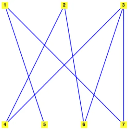
Example 2.34. Consider the graph in Figure 2.8. The degrees for the vertices of this

graph are: (1) v1 = 4 (2) v2 = 3 (3) v3 = 2 (4) v4 = 2 (5) v5 = 1

This leads to the degree sequence: d= (4,3,2,2,1).

1

2

3 4

5

Figure 2.8. The graph above has a degree sequence d = (4,3,2,2,1). These are the degrees of the vertices in the graph arranged in increasing order.

Assumption 1 (Pigeonhole Principle). Suppose items may be classified according to m

possible types and we are given n > m items. Then there are at least two items with the same type.

Remark2.35. The Pigeonhole Principle was originally formulated by thinking of placing

m+ 1 pigeons intompigeon holes. Clearly to place all the pigeons in the holes, one hole has two pigeons in it. The holes are the types (each whole is a different type) and the pigeons are the objects. Another good example deals with gloves: There are two types of gloves (left handed and right handed). If I hand you three gloves (the objects), then you either have two left-handed gloves or two right-handed gloves.

Theorem 2.36. Let G= (V, E) be a non-empty, non-trivial graph. Then G has at least

one pair of vertices with equal degree.

Proof. This proof uses the Pigeonhole Principal and is illustrated by the graph in Figure

2.8, where deg(v3) = deg(v4). The types will be the possible vertex degree values and the

(23)

Suppose _|V_| =n. Each vertex could have a degree between 0 and n₋1 (for a total of

n possible degrees), but if the graph has a vertex of degree 0 then it cannot have a vertex of degree n₋1. Therefore, there are only at most n₋1 possible degree values depending on whether the graph has an isolated vertex or a vertex with degreen₋1 (if it has neither, there are even fewer than n₋1 possible degree values). Thus by the Pigeonhole Principal,

at least two vertices must have the same degree.

Theorem 2.37. Let G= (V, E) be a (general) graph then:

(2.4) 2_|E_|=X

v∈V

deg(v)

Proof. Consider two verticesv1 andv2 inV. If e={v1, v2}then a +1 is contributed to

P

v∈V deg(v) for bothv1 and v2. Thus every non-self-loop edge contributes +2 to the vertex

degree sum. On the other hand, if e = _{v1} is a self-loop, then this edge contributes +2

to the degree of v1. Therefore, each edge contributes exactly +2 to the vertex degree sum.

Equation 2.4 follows immediately.

Corollary 2.38. LetG= (V, E). Then there are an even number of vertices inV with

odd degree.

Exercise 5. Prove Corollary 2.38.

Definition 2.39 (Graphic Sequence). Let d = (d1, . . . , dn) be a tuple in Zn with d1 ≥

d2 ≥ · · · ≥dn. Thend is graphic if there exists a graphG with degree sequence d.

Corollary 2.40. If d is graphic, then the sum of its elements is even.

Exercise 6. Prove Corollary 2.40.

Lemma 2.41. Let d = (d1, . . . , dn) be a graphic degree sequence. Then there exists a

graph G= (V, E) with degree sequence d so that if V =_{v1, . . . , vn} then:

(1) deg(vi) =di for i= 1, . . . , n and

(2) v1 is adjacent to vertices v2, . . . , vd1+1.

Proof. The fact that d is graphic means there is at least one graph whose degree

sequence is equal to d. From among all those graphs, chose G= (V, E) to maximize (2.5) r=_|N(v1)∩ {v2, . . . , vd1+1}|

Recall thatN(v1) is the neighborhood ofv1. Thus maximizing Expression 2.5 implies we are

attempting to make sure that as many vertices in the set _{v2, . . . , vd1+1} are adjacent tov1

as possible.

If r =d1, then the theorem is proved sincev1 is adjacent to v2, . . . , vd1+1. Therefore we’ll

proceed by contradiction and assume r < d1. We know the following things:

(1) Since deg(v1) =d1 there must be a vertex vt with t > d1+ 1 so that vt is adjacent

tov1.

(2) Moreover, there is a vertex vs with 2≤s ≤d1+ 1 that is not adjacent to v1.

(24)

(4) Therefore, there is some vertex vk ∈ V so that vs is adjacent to vk but vt is not

becausevt is adjacent to v1 and vs is not and the degree of vs is at least as large as

the degree ofvt.

Let us create a new graph G0 = (V, E0). The edge set E0 is constructed from E by: (1) Removing edge _{v1, vt}.

(2) Removing edge _{vs, vk}.

(3) Adding edge _{v1, vs}.

(4) Adding edge _{vt, vk}.

This is ilustrated in Figure 2.9. In this construction, the degrees of v1, vt, vs and vk are

d1+ 1 2 3 s t k 1 d1+ 1 2 3 s t k 1

Figure 2.9. We construct a new graph G0 from G that has a larger value r (See Expression 2.5) than our original graph G did. This contradicts our assumption thatG was chosen to maximizer.

preserved. However, it is clear that in G0:

r0 =_|NG0(v₁)∩ {v₂, . . . , v_d

1+1}|

and we haver0 > r. This contradicts our initial choice of G and proves the theorem.

Theorem 2.42 (Havel-Hakimi Theorem). A degree sequenced = (d1, . . . , dn) is graphic

if and only if the sequence (d2−1, . . . , dd1+1−1, dd1+2, . . . , dn) is graphic.

Proof. (⇒) Suppose that d= (d1, . . . , dn) is graphic. Then by Lemma 2.41 there is a

graph Gwith degree sequence d so that: (1) deg(vi) =di for i= 1, . . . , n and (2) v1 is adjacent to vertices v2, . . . , vd1+1.

If we remove vertexv1 and all edges containingv1 from this graph Gto obtainG0 then inG0

for all i= 2, . . . d1+ 1 the degree ofvi is di−1 while forj =d1+ 2, . . . , n the degree of vj is dj because v1 is not adjacent to vd1+2, . . . , vn by choice of G. Thus G

0 _{has degree sequence} (d2−1, . . . , dd1+1−1, dd1+2, . . . , dn) and thus it is graphic.

(_⇐) Now suppose that (d2−1, . . . , dd1+1−1, dd1+2, . . . , dn) is graphic. Then there is some

(25)

adding a vertex v1 to G and creating an edge from v1 to each vertex v2 through vd1+1. It

is clear that the degree of v1 is d1, while the degrees of all other verticesvi must be di and

thus d= (d1, . . . , dn) is graphic because it is the degree sequence ofG0. This completes the

proof.

Remark2.43. Naturally one might have to rearrange the ordering of the degree sequence

(d2−1, . . . , dd1+1−1, dd1+2, . . . , dn) to ensure it is in descending order.

Example 2.44. Consider the degree sequenced= (5,5,4,3,2,1). One might ask, is this

degree sequence graphic. Note that 5 + 5 + 4 + 3 + 2 + 1 = 20 so at least the necessary condition, that the degree sequence sum to an even number is satisfied. In this d we have

d1 = 5, d2 = 5, d3 = 4, d4 = 3, d5 = 2 andd6 = 1.

Applying the Havel-Hakimi Theorem, we know that this degree sequence is graphic if and only if: d0 = (4,3,2,1,0) is graphic. Note, that this is (d2−1, d3−1, d4−1, d5−1, d6−1)

since d1+ 1 = 5 + 1 = 6. Now, if d0 where graphic, then we would have a graph with 5

vertices one of which has degree 4 and another that has degree 0 and no to vertices have the same degree. Applying either Theorem 2.36 (or its proof), we see this is not possible. Thus

d0 is not graphic and so d is not graphic.

Exercise 7. Develop a (recursive) algorithm based on Theorem 2.42 to determine

whether a sequence is graphic. [Hint: See Page 10 of [GY05].]

Theorem 2.45 (Erd¨os-Gallai Theorem2). A degree sequence d= (d1, . . . , dn) is graphic

if and only if its sum is even and for all 1_≤k _≤n₋1:

(2.6) k X i=1 di ≤k(k+ 1) + n−1 X i=k+1 min_{k+ 1, di}

Exercise 8 (Independent Project). There are several proofs of Theorem 2.45, some

short. Investigate them and reconstruct an annotated proof of the result. In addition investigate Berg’s approach using flows [Ber73].

Remark 2.46. There has been a lot of interest recently in degree sequences of graphs,

particularly as a result of the work in Network Science on so-calledscale-free networks. This has led to a great deal of investigation into properties of graphs with specific kinds of degree sequences. For the brave, it is worth looking at [MR95], [ACL01], [BR03] and [Lu01] for interesting mathematical results in this case. To find out why all this investigation started, see [BAJB00].

3.1. Types of Graphs from Degree Sequences.

Definition 2.47 (Complete Graph). Let G = (V, E) be a graph with |V| = n with

n _≥ 1. If the degree sequence of G is (n₋1, n₋1, . . . , n₋1) then G is called a complete graph on n vertices and is denoted Kn. In a complete graph on n vertices each vertex is

connected to every other vertex by an edge.

2_{Thanks to an anonymous comment from the Internet, that detected a small typo in Equation 2.6 in}

(26)

Lemma 2.48. Let Kn = (V, E) be the complete graph on n vertices. Then:

|E_|= n(n−1) 2

Corollary 2.49. Let G= (V, E) be a graph and let |V|=n. Then:

0_{≤ |}E_{| ≤} n 2

Exercise 9. Prove Lemma 2.48 and Corollary 2.49. [Hint: Use Equation 2.4.]

Definition 2.50 (Regular Graph). Let G = (V, E) be a graph with |V| = n. If the

degree sequence of G is (k, k, . . . , k) withk _≤n₋1 then Gis called a k-regular graph on n

vertices.

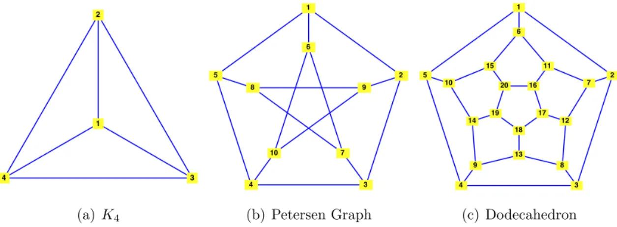
Example2.51. We illustrate one complete graph and two (non-complete) regular graphs

in Figure 2.10. Obviously every complete graph is a regular graph. Every Platonic solid is

(a) K4 (b) Petersen Graph (c) Dodecahedron

Figure 2.10. The complete graph, the “Petersen Graph” and the Dodecahedron. All Platonic solids are three-dimensional representations of regular graphs, but not all regular graphs are Platonic solids. These figures were generated with Maple.

also a regular graph, but not every regular graph is a Platonic solid. In Figure 2.10(c) we show a flattened dodecahedron, one of the five platonic solids from classical geometry. The Peteron Graph (Figure 2.10(b)) is a 3-regular graph that is used in many graph theoretic examples.

3.2. Digraphs.

Definition 2.52 (In-Degree, Out-Degree). LetG= (V, E) be a digraph. The in-degree

of a vertex v in G is the total number of edges in E with destination v. The out-degree of

v is the total number of edges in E with source v. We will denote the in-degree of v by deg_in(v) and the out-degree by deg_out(v).

(27)

Theorem 2.53. Let G= (V, E) be a digraph. Then the following holds: (2.7) _|E_|=X v∈V deg_in(v) = X v∈V deg_out(v)

Exercise 10. Prove Theorem 2.53.

4. Subgraphs

Definition 2.54 (Subgraph). Let G= (V, E). A graph H= (V0, E0) is a subgraph of G

if V0 _⊆V and E0 _⊆E. The subgraph H is proper if V0 ₍V or E0 ₍E.

Example2.55. We illustrate the notion of a sub-graph in Figure 2.11. Here we illustrate

a sub-graph of the Petersen Graph. The sub-graph contains vertices 6, 7, 8, 9 and 10 and the edges connecting them.

(a) Petersen Graph (b) Highlighted Subgraph (c) Extracted Subgraph Figure 2.11. The Petersen Graph is shown (a) with a sub-graph highlighted (b) and that sub-graph displayed on its own (c). A sub-graph of a graph is another graph whose vertices and edges are sub-collections of those of the original graph.

Definition 2.56 (Spanning Subgraph). LetG= (V, E) be a graph andH = (V0, E0) be

a subgraph of G. The subgraph H is a spanning subgraph of Gif V0 =V.

Definition 2.57 (Edge Induced Subgraph). LetG= (V, E) be a graph. IfE0 ⊆E. The

subgraph ofGinduced by E0 is the graphH = (V0, E0) wherev _∈V0 if and only ifv appears in an edge inE.

Definition 2.58 (Vertex Induced Subgraph). Let G = (V, E) be a graph. If V0 ⊆ E.

The subgraph of G induced byV0 is the graphH = (V0, E0) where _{v1, v2} ∈E0 if and only

if v1 and v2 are both in V0.

Remark 2.59. For directed graphs, all sub-graph definitions are modified in the obvious

(28)

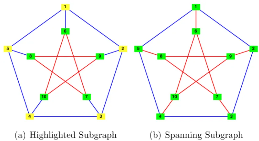
Example 2.60. Using the Petersen Graph we illustrate a subgraph induced by a vertex

subset and a spanning subgraph. In Figure 2.12(a) we illustrate the subgraph induced by the vertex subset V0 =_{6,7,8,9,10_} (shown in red). In Figure 2.12(b) we have a spanning subgraph induced by the edge subset:

E0 =_{{1,6_},_{2,9_},_{3,7_},_{4,10_},_{5,8_},_{6,7_},_{6,10_},_{7,8_},_{8,9_},_{9,10_}}

(a) Highlighted Subgraph (b) Spanning Subgraph

Figure 2.12. The subgraph (a) is induced by the vertex subsetV0 ={6,7,8,9,10}. The subgraph shown in (b) is a spanning sub-graph and is induced by edge subset

E0 ={{1,6},{2,9},{3,7},{4,10},{5,8},{6,7},{6,10},{7,8},{8,9},{9,10}}.

5. Graph Complement, Cliques and Independent Sets

Definition 2.61 (Clique). Let G = (V, E) be a graph. A clique is a set S ⊆ V of

vertices so that:

(1) The subgraph induced byS is a complete graph (or in general graphs, every pair of vertices in S is connected by at least one edge in E)and

(2) If S0 _⊃ S, there is at least one pair of vertices in S0 that are not connected by an edge inE.

Definition 2.62 (Independent Set). Let G = (V, E) be a graph. A independent set of

G is a setI _⊆V so that no pair of vertices in I is joined by an edge in E. A set I _⊆V is a

maximal independent set if I is independent and if there is no other setJ _⊃ I such that J

is also independent.

Example 2.63. The easiest way to think of cliques is as subgraphs that are Kn but

so that no larger set of vertices induces a larger complete graph. Independent sets are the opposite of cliques. The graph illustrated in Figure 2.13(a) has 3 cliques. An independent set is illustrated in Figure 2.13(b).

Definition 2.64 (Clique Number). Let G = (V, E) be a graph. The clique number of

(29)

(a) Cliques (b) Independent Set

Figure 2.13. A clique is a set of vertices in a graph that induce a complete graph as a subgraph and so that no larger set of vertices has this property. The graph in this figure has 3 cliques.

Definition 2.65 (Independence Number). The independence number of a graph G =

(V, E), written α(G), is the size of the largest independent set ofG.

Exercise 11. Find the clique and independence numbers of the graph shown in Figure

2.13(a)/(b).

Definition 2.66 (Graph Complement). Let G= (V, E) be a graph. The graph

comple-ment of Gis a graph H = (V, E0) so that:

e=_{v1, v2} ∈E0 ⇐⇒ {v1, v2} 6∈E

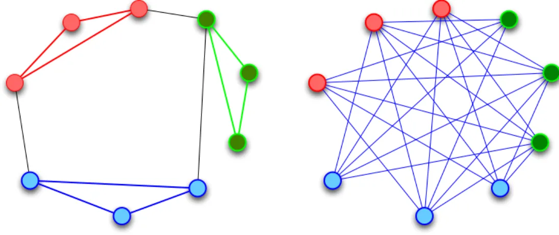
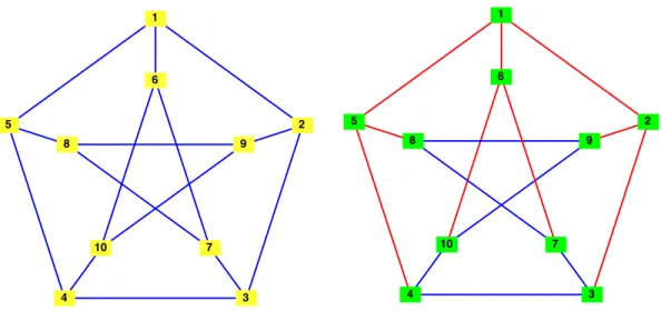
Example 2.67. In Figure 2.14, the graph from Figure 2.13 is illustrated (in a different

spatial configuration) with its cliques. The complement of the graph is also illustrated. Notice that in the complement, every clique is now an independent set.

Figure 2.14. A graph and its complement with cliques in one illustrated and in-dependent sets in the other illustrated.

(30)

Definition 2.68 (Relative Complement). IfG= (V, E) is a graph and H = (V, E0) is a

spanning sub-graph, then therelative complement ofH inGis the graphH0 = (V, E00) with:

e=_{v1, v2} ∈E00 ⇐⇒ {v1, v2} ∈E and {v1, v2} 6∈E0

Theorem 2.69. LetG= (V, E)be a graph and let H = (V, E0) be its complement. A set

S is a clique in G if and only if S is a maximal independent set in H.

Exercise 12. Prove Theorem 2.69. [Hint: Use the definition of graph complement and

the fact that if an edge is present in a graph G is must be absent in its complement.]

Definition 2.70 (Vertex Cover). LetG= (V, E) be a graph. A vertex cover is a set of

verticesS _⊆V so that for all e_∈E at least one element ofe is in S; i.e., every edge inE is adjacent to at least one vertex in S.

Example 2.71. A covering is illustrated in Figure 2.15

Figure 2.15. A covering is a set of vertices so that ever edge has at least one endpoint inside the covering set.

Exercise 13. Illustrate by exhaustion that removing any vertex from the proposed

covering in Figure 2.15 destroys the covering property.

Theorem 2.72. A set I is an independent set in a graph G= (V, E) if and only if the

set V _\I is a covering in G.

Proof. (⇒) Suppose that I is an independent set and choose e={v, v0} ∈E. If v ∈I,

then clearly v0 _∈ V _\I. The same is true of v0. It is possible that neither v nor v0 is in I, but this does not affect that fact that V _\I must be a cover since for every edge e _∈ E at least one element is in V _\I.

(_⇐) Now suppose thatV _\I is a vertex covering. Choose any two vertices v and v0 inI. The fact thatV _\I is a vertex covering implies that _{v, v0_} cannot be an edge inE because it does not contain at least one element from V _\I, contradicting our assumption on V _\I. Thus,I is an independent set since no two vertices in I are connected by an edge inE. This

(31)

Remark2.73. Theorem 2.72 shows that the problem of identifying a largest independent

set is identical to the problem of identifying a minimum (size) vertex covering. As it turns out, both these problems are equivalent to yet a third problem, which we will discuss later called the matching problem. Coverings (and matchings) are useful, but to see one example of their utility imagine a network of outposts is to be established in an area (like a combat theatre). We want to deliver a certain type of supplies (antibiotics for example) to the outposts in such a way so that no outpost is anymore than one link (edge) away from an outpost where the supply is available. The resulting problem is a vertex covering problem. In attempting to find the minimal vertex covering asks the question what is the minimum number of outposts that must be given antibiotics?

(32)

(33)

CHAPTER 3

More Definitions and Theorems

1. Paths, Walks, and Cycles

Definition3.1 (Walk).LetG= (V, E) be a graph. A walkw= (v1, e1, v2, e2, . . . , vn, en, vn+1)

inG is an alternating sequence of vertices and edges inV and E respectively so that for all

i= 1, . . . , n: _{vi, vi+1}=ei. A walk is calledclosed ifv1 =vn+1 andopen otherwise. A walk

consisting of only one vertex is calledtrivial.

Definition 3.2 (Sub-Walk). Let G = (V, E) be a graph. If w is a walk in G then a

sub-walk of w is any walk w0 that is also a sub-sequence ofw.

Remark 3.3. Let G = (V, E) to each walk w = (v1, e1, v2, e2, . . . , vn, en, vn+1) we can

associated a subgraphH = (V0, E0) with: (1) V0 =_{v1, . . . , vn+1}

(2) E0 =_{e1, . . . , en}

We will call this the sub-graph induced by the walk w.

Definition 3.4 (Trail/Tour). Let G = (V, E) be a graph. A trail in G is a walk in

which no edge is repeated. Atour is a closed trail. An Eulerian trail is a trail that contains exactly one copy of each edge inE and anEulerian tour is a closed trail (tour) that contains exactly one copy of each edge.

Definition 3.5 (Path). Let G= (V, E) be a graph. A path in G is a non-trivial walk

with no vertex and no edge repeated. A Hamiltonian path is a path that contains exactly one copy of each vertex in V1_.

Definition 3.6 (Length). The length of a walk w is the number of edges contained in

it.

Definition 3.7 (Cycle). A closed walk of length at least 3 and with no repeated edges

and in which the only repeated vertices are the first and the last is called a cycle. A

Hamiltonian cycle is a cycle in a graph containing every vertex.

Definition 3.8 (Hamiltonian / Eulerian Graph). A graph G = (V, E) is said to be

Hamiltonian if it contains a Hamiltonian cycle and Eulerian if it contains an Eulerian tour.

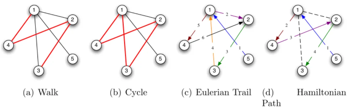
Example 3.9. We illustrate a walk, cycle, Eulerian tour and a Hamiltonian path in

Figure 3.1.

A walk is illustrated in Figure 3.1(a). Formally, this walk can be written as:

w= (1,_{1,4_},4,_{4,2_},2,_{2,3_},3)

(34)

1 2 3 4 5 (a) Walk 1 2 3 4 5 (b) Cycle 1 2 3 4 5 1 2 3 4 5 6 (c) Eulerian Trail 1 2 3 4 5 1 4 2 3 (d) Hamiltonian Path

Figure 3.1. A walk (a), cycle (b), Eulerian trail (c) and Hamiltonian path (d) are illustrated.

The cycle shown in Figure 3.1(b) can be formally written as:

c= (1,_{1,4_},4,_{4,2_},2,_{2,3_},3,_{3,1_},1)

Notice that the cycle begins and ends with the same vertex (that’s what makes it a cycle). Also,w is a sub-walk of c. Note further we could easily have represented the walk as:

w= (3,_{3,2_},2,_{2,4_},4,_{4,1_},1)

We could have shifted the ordering of the cycle in anyway (for example beginning at vertex 2). Thus we see that in an undirected graph, a cycle or walk representation may not be unique.

In Figure 3.1(c) we illustrate an Eulerian Trail. This walk contains every edge in the graph with no repeats. We note that Vertex 1 is repeated in the trail, meaning this is not a path. We contrast this with Figure 3.1(d) which shows a Hamiltonian path. Here each vertex occurs exactly once in the illustrated path, but not all the edges are included. In this graph, it is impossible to have either a Hamiltonian Cycle or an Eulerian Tour.

Exercise 14. Prove it is not possible for a Hamiltonian Cycle or Eulerian Tour to exist

in the graph in Figure 3.1(a); i.e., prove that the graph is neither Hamiltonian nor Eulerian.

Remark 3.10. If w is a path in a graphG= (V, E) then the subgraph induced by w is

simply the graph composed of the vertices and edges in w.

Proposition3.11. LetGbe a graph and let wbe an Eulerian trail (or tour) in G. Then

the sub-graph of G induced by w is G itself when G has no isolated vertices.

Exercise 15. Prove Proposition 3.11.

Definition 3.12 (Path / Cycle Graph). Suppose that G = (V, E) is a graph with

|V_|=n. If w is a Hamiltonian path in Gand H is the subgraph induced by w and H =G, then G is called a n-path or a Path Graph on n vertices denoted Pn. If w is a Hamiltonian cycle in Gand H is the subgraph induced by wand H =G, thenG is called a n-cycle or a

Cycle Graph on n vertices denoted Cn.

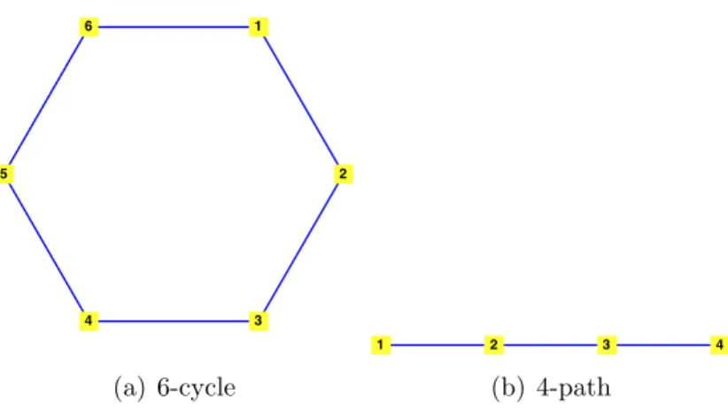
Example 3.13. We illustrate a cycle graph with 6 vertices (6-cycle or C6) and a path

(35)

(a) 6-cycle (b) 4-path Figure 3.2. We illustrate the 6-cycle and 4-path.

Remark 3.14. For the most part, the terminology on paths, cycles, tours etc. is

stan-dardized. However, not every author adheres to these same terms. It is always wise to identify exactly what words an author is using for walks, paths cycles etc.

Remark3.15. Walks, cycles, paths and tours can all be extended to the case of digraphs.

In this case, the walk, path, cycle or tour must respect the edge directionality. Thus, if

w= (. . . , vi, ei, vi+1, . . .) is a directed walk, then ei = (vi, vi+1) as an ordered pair.

Exercise16. Formally define directed walks, directed cycles, directed paths and directed

tours for directed graphs. [Hint: Begin with Definition 3.1 and make appropriate changes. Then do this for cycles, tours etc.]

2. More Graph Properties: Diameter, Radius, Circumference, Girth

Definition 3.16 (Distance). Let G = (V, E). The distance between v1 and v2 in V

is the length of the shortest walk beginning at v1 and ending at v2 if such a walk exists.

Otherwise, it is +_∞. We will write dG(v1, v2) for the distance from v1 to v2 in G.

Definition 3.17 (Directed Distance). Let G = (V, E) be a digraph. The (directed)

distance between v1 to v2 in V is the length of the shortest directed walk beginning at v1

and ending at v2 if such a walk exists. Otherwise, it is +∞

Definition 3.18 (Diameter). Let G= (V, E) be a graph. The diameter of G diam(G)

is the length of the largest distance in G. That is: (3.1) diam(G) = max

v1,v2∈V

dG(v1, v2)

Definition 3.19 (Eccentricity). LetG = (V, E) and let v1 ∈V. The eccentricity of v1

is the largest distance fromv1 to any other vertexv2 inV. That is:

(3.2) ecc(v1) = max

v2∈V

dG(v1, v2)

Exercise 17. Show that the diameter of a graph is in fact the maximum eccentricity of

(36)

Definition 3.20 (Radius). Let G= (V, E). The radius of G is minimum eccentricy of

any vertex in V. That is: (3.3) rad(G) = min v1∈V ecc(v1) = min v1∈V max v2∈V dG(v1, v2)

Definition 3.21 (Girth). Let G = (V, E) be a graph. If there is a cycle in G (that is

G has a cycle-graph as a subgraph), then the girth of G is the length of the shortest cycle. When G contains no cycle, the girth is defined as 0.

Definition 3.22 (Circumference). Let G = (V, E) be a graph. If there is a cycle in G

(that isGhas a cycle-graph as a subgraph), then the circumference of Gis the length of the

longest cycle. WhenG contains no cycle, the circumference is defined as +_∞.

Example 3.23. The eccentricities of the vertices of the graph shown in Figure 3.3 are:

(1) Vertex 1: 1 (2) Vertex 2: 2 (3) Vertex 3: 2 (4) Vertex 4: 2 (5) Vertex 5: 2

This means that the diameter of the graph is 2 and the radius is 1. We have already seen that there is a 4-cycle subgraph in the graph (see Figure 3.1(b)). This is the largest cycle in the graph, so the circumference of the graph is 4. There are several 3-cycles in the graph (an example being the cycle (1,_{1,2_},2,_{2,4_},4,_{4,1_},1)). The smallest possible cycle is a 3-cycle. Thus the girth of the graph is 3.

1

2

3 4

5

Figure 3.3. The diameter of this graph is 2, the radius is 1. It’s girth is 3 and its circumference is 4.

Exercise 18. Compute the diameter, radius, girth and circumference of the Petersen

Graph.

3. More on Trails and Cycles

Remark 3.24. Suppose that

w= (v1, e1, v2, . . . , vn, en, vn+1)

If for somem _{∈ {}1, . . . , n_} and for some k _∈_Zwe have vm =vm+k. Then w0 = (vm, em, . . . , em+k−1, vm+k)

is aclosed sub-walk of w. The walkw0 can be deleted from the walkwto obtain a new walk: