When is monetary policy all we need?

(1)

When is Monetary Policy All we Need?

∗ Fabian Eser†, Campbell Leith‡ & Simon Wren-Lewis§

8th May 2009

Abstract

We consider optimal monetary and fiscal policies in a New Keynesian model of a small open economy with sticky prices and wages. In this benchmark setting monetary policy is all we need - analytical results demonstrate that variations in government spending should play no role in the stabilization of shocks. In extensions we show, firstly, that this is even when true when allowing for inflation inertia through backward-looking rule-of-thumb price and wage-setting, as long as there is no discrepancy between the private and social evaluation of the marginal rate of substitution between consumption and leisure. Secondly, the optimal neutrality of government spending is robust to the issuance of public debt. In the presence of debt government spending will deviate from the optimal steady-state but only to the extent required to cover the deficit, not to provide any additional macroeconomic stabilization. However, unlike government spending variations in tax rates can play a complementary role to monetary policy, as they change relative prices rather than demand.

Keywords: Monetary Policy, Fiscal Policy, Macroeconomic Stabilization, Dynamic General Equilibrium, Sticky Prices, Sticky wages, Rule-of-Thumb Behaviour, Debt, Countercyclical Policy

JEL Classification: E5, E6, C62

∗

We would like to thank Andrew Hughes-Hallett, Tatiana Kirsanova, Patrick Minford, Charles Nolan, Bianca De Paoli, Jari Stehn, Alan Sutherland, David Vines, Mike Wickens, participants at seminars at the Centre for Economic Policy, LSE, HM Treasury, St Andrews, and Oxford Universities, a Money Macro and Finance workshop and a conference at the National Bank of Belgium for very helpful discussions on an earlier version of this paper. All errors remain our own. Leith and Wren-Lewis are also grateful to the ESRC, Grant 156-25-003 and RES-062-23-1436, for financial assistance, while Eser thanks the ESRC and the Royal Economic Society for financial assistance. Address for correspondence: Campbell Leith, Department of Economics, University of Glasgow, Adam Smith Building, Glasgow G12 8RT.

†

University of Oxford,fabian.eser@nuffield.ox.ac.uk.

‡

University of Glasgow,c.b.leith@lbss.gla.ac.uk.

§

(2)

1 Introduction

We address the issue of whether fiscal policy should be used as a demand management tool when monetary policy is set in an optimal and unconstrained manner. As recent events have shown, there remain occasions in which policymakers wish to supplement monetary policy with fiscal action to control the business cycle, but these actions remain controversial among macroeconomists. In the main part of this paper we focus on fiscal policy as a tool for influencing aggregate demand, as opposed to a means of changing relative prices. To do this we use government spending as our fiscal instrument, although we note towards the end how some results would change if taxes were the fiscal instrument.

We begin by setting out a baseline model that combines what are generally regarded as core features of New Keynesian models: imperfectly competitive firms subject to Calvo contracts, house-holds making optimal, intertemporal choices over consumption and labour supply, and a social wel-fare function derived from their utility. In addition, we introduce a nominal wage rigidity as this adds both realism and removes the ability of monetary policy to completely offset the impact of technology and preference shocks. Analytical results show that changes in the government spend-ing gap should not be used to supplement optimal monetary policy under either commitment or discretion, whether shocks come from technology, changes in preferences or are mark-up shocks.1 In this sense fiscal policy should not be used for aggregate demand management when monetary policy is unconstrained.

We then consider how robust these results might be to two extensions of the model. A common theme of empirical studies is that the economy is subject to some degree of inflation inertia, in the sense that lagged inflation appears alongside expected inflation in the Phillips curve. We model this with backward-looking rule of thumb-behaviour of both wage- and price-setters. Importantly, we show that government spending still has no role to play in stabilization if there is no endogenous wedge between the marginal rate of substitution between consumption and leisure as seen by the social planner and wage setters. For if such a wedge exists the policymaker could use the government

1_{The closed economy case with flexible wages is examined in detail in}_Eser₍₂₀₀₉_{), which is a revised and extended} version ofEser(2006).

(4)

spending gap to exploit this difference in wage/price setting.

Our baseline model also ignores debt. Once we allow shocks to change the stock of government debt in the absence of lump sum taxes, the optimal government spending gap is no longer zero. However we show that this gap moves to a new, constant level designed to finance higher debt, and therefore does not play a countercyclical role. Finally we discuss the extent to which these results apply only to government spending as an instrument, representing a demand management role for fiscal policy. We show that variations in tax rates, by changing relative prices, can play a complementary role to monetary policy.

It is important to restate that we restrict ourselves to settings where monetary policy is un-constrained in the sense that there is no direct cost in varying interest rates to influence aggregate demand and we ignore the possibility of interest rates hitting a zero lower bound, a consideration that might well justify a fiscal response to severe deflation. In addition if, for some reason, mone-tary policy was constrained to follow a simple form of Taylor rule, then this could reprise a role for fiscal demand management (see Eser (2009) but also Schmitt-Groh´e and Uribe (2007)). We also ignore frictions on the monetary side. These are considered inEser(2009) which shows that a fiscal stabilization role can arise if monetary frictions exist, even when monetary policy is set optimally. The main reason for this is that in that under monetary frictions variations of the interest rate directly lead to a social loss of second order. Furthermore, we exclude any uncertainty about the transmission mechanism of monetary policy. While all these considerations may be important in practice, the case where monetary policy is optimal and unconstrained seems like a natural starting point for analysis.

2 Baseline Model

This section outlines our baseline model. It is for a small open economy where consumers have a bias to purchase domestically produced goods, which has the advantage that a closed economy is a special case of the model where this home bias is complete. The model is similar in structure to Gal´ı and Monacelli (2005), with the main addition being the presence of sticky wages as well

(5)

as sticky prices. The core ingredients of the closed economy version of the model - intertemporal optimisation by consumers over goods and leisure and Calvo contracts - are common to a large number of papers in the literature.

2.1 Households

There are a continuum of households of size one, who differ in that they provide differentiated labour services to firms in their economy. However, we shall assume full asset markets, such that, through risk sharing, they will face the same budget constraint and make the same consumption plans even if they face different wage rates due to stickiness in wage-setting. We assume the typical household maximises the following objective function

E0 ∞ X t=0 βt lnCt+χlnGt− Nt(k)1+ϕ 1 +ϕ , (1)

where Ct, Gt and Nt are a consumption aggregate, a public goods aggregate, and labour supply

respectively. χdenotes the relative weight of government spending in the utility function. The only notation referring to the specific household k indexes the labour input, as full financial markets will imply that all other variables are constant across households. The consumption aggregate is defined asCt=

C_H,t1−αCα F,t

(1−α)(1−α)_αα. The composite of domestically produced goods is given by

CH,t= ( Z 1 0 CH,t(j) −1 dj) −1 ₍₂₎

where j denotes the good’s variety. The aggregate CF,t is an aggregate across countries i CF,t =

(R1 0 C γ−1 γ i,t di) γ γ−1_{, where}_C

i,tis an aggregate similar to (2). γmeasures the substitutability between

goods produced in different foreign countries. For convenience we assumeγ = 1 in what follows.

This assumption, together with international risk sharing discussed below, helps make aspects of open economy problem isomorphic to the closed economy, which greatly simplifies the analysis (see

Benigno and De Paoli (2009) and Kirsanova et al. (2006). Finally, the public goods aggregate is given by Gt = ( R1 0 Gt(j) −1 dj)

−1_{, which implies that public goods are all domestically produced.}

(6)

The parameterαis (inversely) related to the degree of home bias in preferences, and is a natural measure of openness. If α = 1 we have no home bias, and the only potential connection between domestic consumption and domestic output is through income, although this is in turn modified by international risk sharing, which we discuss below. If α= 0 we have a closed economy.

The budget constraint at time tis given by

Πt+Dt+Wt(k)Nt(k)(1−τt)−Tt = Z 1 0 PH,t(j)CH,t(j)dj+ Z 1 0 Z 1 0

Pi,t(j)Ci,t(j)djdi+Et{Qt,t+1Dt+1},

wherePi,t(j) is the price of varietyj imported from countryiexpressed in home currency, Dt+1 is

the nominal payoff of the portfolio held at the end of periodt, Πtis the representative household’s

share of profits in the imperfectly competitive firms, W are wages, τt is an wage income tax rate,

and Tt are lump sum taxes. Qt,t+1 is the stochastic discount factor for one period ahead payoffs.

Households first decide how to allocate a given level of expenditure across the various goods that are available, minimising the cost of consumption. Optimisation of expenditure for any individual good implies the demand functions

CH,t(j) = PH,t(j) PH,t − CH, Ci,t(j) = Pi,t(j) Pi,t − Ci,t.

The associated price indices are given by

PH,t= Z 1 0 PH,t(j)1−dj 1−1 , Pi,t = Z 1 0 Pi,t(j)1−dj 1−1 .

It follows that R₀1PH,t(j)CH,t(j)dj = PH,tCH,t and R1

0 Pi,t(j)Ci,t(j)dj = Pi,tCi,t. Optimisation

across imported goods by country implies R1

0 Pi,tCi,tdi = PF,tCF,t. Defining the consumer price

index (CPI) as

Pt=PH,t1−αPF,tα , (3)

(7)

and PF,tCF,t=αPtCt. With these results the budget constraint can be written as

PtCt+Et{Qt,t+1Dt+1}= Πt+Dt+Wt(k)Nt(k)(1−τt)−Tt. (4)

The first of the household’s intertemporal problems involves allocating consumption expenditure across time. This implies

βRtEt Ct Ct+1 Pt Pt+1 = 1, (5)

whereRt= _E_t_{_Q1_t,t₊₁_} is the gross return on a riskless one period bond paying off a unit of domestic

currency int+ 1. A log-linearised version of (5) can be written as

ct=Et{ct+1} −(rt−Et{πt+1} −ρ), (6)

where lowercase denotes logs,ρ = 1_β−1. Consumer price inflation (CPI) is defined asπt≡pt−pt−1.

The modelling of households’ wage-setting behaviour essentially follows Erceg et al. (2000). They apply Calvo pricing to wage setting. We assume that firms need to employ a CES aggregate of the labour of all households in the domestic production of consumer goods. This is provided by an ‘aggregator’ that aggregates the labour services of all households in the economy as

Nt= Z 1 0 Nt(k) w−1 w _dk _ww−1 ,

where Nt(k) is the labour provided by household k to the aggregator. We allow the degree of

labour differentiation to vary in response to independent and identically distributed random shocks which introduce the possibility of wage mark-up shocks. Accordingly the demand curve facing each household is given by Nt(k) = Wt(k) Wt −w Nt, (7)

whereNt, the CES aggregate of labour services in the economy, also equals the total labour services

employed by firms: Nt = R1

0 Nt(j) dj, where Nt(j) is the labour employed by firm j. The price

of this labour is given by the wage index Wt= h

R1

0 Wt(k) 1−w_dk

i1−w

(8)

function for the setting of its nominal wage is given by Et "_∞ X s=0 (θwβ)s Λt+s Wt(k) Pt+s (1−τt+s)Nt+s(k)− (Nt+s(k))1+ϕ 1 +ϕ # , (8)

where Λt+s=Ct−+1sis the marginal utility of real post-tax income, and 1−θwis the probability that

nominal wages change in a given period. As detailed in appendixA.2, the first order condition from this problem can be combined with the aggregate wage index to give a log-linearised expression for wage-inflation dynamics, π_tw =βEtπwt+1+ λw 1 +ϕw (ϕnt−(wt−pt) +ct−ln(1−τt) +µwt ) (9) where λw = (1 −θwβ)(1−θw) θw and e µw

t is the desired wage-markup in the absence of wage stickiness,

which fluctuates around w

w−1 in response to iid wage mark-up shocks. The forcing variable in this

New Keynesian Phillips curve (NKPC) is a log-linearised measure of the extent to which wages are not at the level implied by the labour supply decision that would hold under flexible wages.

The allocation of government spending across goods is determined by minimising total costs,

R1

0 PH(j)G(j)dj. Given the form of the basket of public goods this implies Gt(j) =

_P_H,t(_j₎ PH,t

−

Gt.

2.2 The exchange rate and risk sharing

The bilateral terms of trade are the price of country i’s goods relative to home goods prices, and is given bySi,t ≡ _PP_H,ti,t. Thus, the effective terms of trade relative to the rest of the world are given

by

S_t= PF,t PH,t

. (10)

Combining (10) with (3), the domestic CPI, producer prices and the effective terms of trade can be related in terms of logs as

pt=pH,t+αst. (11)

Trade in goods is assumed to be free and costless. Thus, the law of one price holds for individual goods at all times. This implies P (j) = E Pi (j) for all i, j ∈ [0,1], where E is the bilateral

(9)

nominal exchange rate. P_i,ti (j) is the price of county i’s good j expressed in terms of country i’s currency. Aggregating across goods implies Pi,t = Ei,tPi,ti , where Pii ≡

R1 0 P i i(j)1−dj ₁₋1 . From the definition of PF,t we have, log-linearised around the symmetric steady state, pF,t = R1 0(ei,t+p i i,t)di=et+p ∗ t, where et= R1

0 ei,tdiis the log of the nominal effective exchange rate, p

i i,t

is the logged domestic price index for country i, and p∗_t = R₀1pi_i,t di is the log of the world price index.

Combining the definition of the terms of trade and the result just obtained givesst=et+p∗t−

pH,t. The bilateral real exchange rate is defined as

Qi,t ≡

Ei,tPi,t

Pt

, (12)

where Pi,t and Pt are the two countries’ respective CPI levels. In logged form we can define the

real effective exchange rate as

qt= Z 1

0

(ei,t+pit−pt) di= (1−α)st. (13)

We assume a perfect international insurance markets for national income risk, so complete interna-tional risk-sharing holds. For the representative household in any other country i a consumption Euler equation holds

βRtEt C_ti C_ti₊₁ P_ti P_ti₊₁ Ei,t E_i,t₊₁ = 1. (14)

Combining (5), (14) and (12) we obtainQ_i,t₊₁Cti+1

Ct+1

=Q_i,tCti

Ct

. This can be iterated backwards so that Ct =zti−1CtiQi,t, where zit−1 ≡ Qi,t−1

Ci t−1

Ct−1 depends on the initial relative net asset

condi-tions. If net foreign asset holdings are zero and the environments identical ex ante, i.e. the initial conditions are symmetric, then z_ti−1 = 1. Then the bilateral risk-sharing condition is Ct=CtiQi,t.

Log-linearising this, integrating over all countries i and using (13) the condition characterising international risk-sharing (IRS) with the rest of the world is

(10)

wherec∗_t is the average level of consumption in the rest of the world.

2.3 Firms

2.3.1 Technology

Firms face the demand curve Yt(j) =

_P_H,t(_j₎ PH,t − (1−α)PtCt PH,t +α R1 0 εiPtiCit PH,t di+Gt , which we rewrite as Yt(j) = _P_H,t(_j₎ PH,t −

Yt, where aggregate output is defined as

Yt≡ Z 1 0 Yt(j) −1 dj ₋₁ . (16)

For any firm j the production function is linear, Yt(j) = AtNt(j), where At is a stochastic

technology-shock. The aggregate of the individual firms’ demand for labour is

Nt= Z 1 0 Nt(i) di= Yt At ∆t, (17)

where price dispersion is defined as ∆t≡ R1 0 _P (H,t)(i) P(H,t) −

di. As shown, for instance, inWoodford

(2003), variations of ∆t around the steady-state are of second-order importance. Thus, to a

first-order (17) can be approximated as

yt=at+nt. (18)

2.3.2 Price-Setting

The objective function of the firm is given by

Et "_∞ X s=0 (θ)sQt,t+s (1−τ_ts₊_s)PH,t(j) Pt+s Yt+s(j)−(1−κ)Wt+s Pt+s Yt+s(j) At+s # , (19)

where κ is an employment subsidy which can be used to eliminate the steady-state distortion

associated with monopolistic competition and distortionary production and income taxes, assuming there is a lump-sum tax available to finance such a subsidy. τ_tsis a production tax. As labour is the only factor of production in this model, the production tax is equivalent to a variable employment

(11)

subsidy. In a closed economy, the production tax is equivalent to a sales tax. 1−θis the probability of a price change in a given period. As shown in appendix A.1 optimisation implies the New Keynesian Phillips Curve (NKPC)

πH,t=βEtπH,t+1+λ(mct+µt), (20)

where λ= (1−θβ_θ)(1−θ) ,mct=wt−pH,t−at−ln(1−τts)−vt are the real log-linearised marginal

costs of production,v=−ln(1−_κ) andeµt _{is the desired mark-up which fluctuates around}

−1 is

response to iid shocks.

2.4 Equilibrium

Goods market clearing requires, for each good j, Yt(j) = CH,t(j) + R1

0 C

i

H,t(j)di+Gt(j).

Sym-metrical preferences imply C_H,ti (j) = α(PH,t(_P j)

H,t )

−PH,t

Ei,tPti

−1

C_ti which allows us to write Yt(j) = _P_H,t(_j₎ PH,t − (1−α)PtCt PH,t +α R1 0 Ei,tPtiCti PH,t di+Gt . Using (16) we obtainYt= (1−α)P_PtCt H,t+α R1 0( εiPtiCti PH,t )di+

Gt, which can be written as

Yt=CtStα+Gt (21)

Then (21) can be written to a first order approximation as

yt= (1−γ) (ct+αst) +γgt, (22)

where γ = G_Y is the steady-state share of government spending in output, which is related to structural model parameters below. To obtain the world wide goods market clearing condition we can simply integrate over (22) to obtain y∗_t = (1−γ)c∗_t +γg∗_t.

Defining the real wage as ωt≡wt−pH,t, (20) can be written as Phillips Curve (NKPC) which

is given by

πH,t=βEtπH,t+1+λ(ωt−at−ln(1−τts)−v+µt) (23)

As shown above, wage inflation dynamics follow (9). The forcing variable captures the extent to which the consumer’s labour supply decision is not the same as it would be under flexible wages.

(12)

Using (11), (22) and (18), (9) can be written as πw_t =βEtπtw+1+ ˜λw ϕ+ 1 1−γ yt− γ 1−γgt−ωt−ϕat−ln(1−τt) +µ w t , (24)

where ˜λw ≡ ₁₊λ_ϕw_w. Finally substituting (11), (22) in (5), we obtain an IS-relation as

yt=Etyt+1−γ∆Etgt+1−(1−γ) (rt−EtπH,t+1−ρ). (25)

3 Optimal policy in the Benchmark Model

3.1 The Social Planner’s Problem

To develop an objective function with which to evaluate optimal policy it is helpful to begin by analysing the social planner’s problem. The social planner simply decides how to allocate consumption and production of goods within the economy, subject to the various constraints implied by operating as part of a larger group of economies. Since they are concerned with real allocations, the social planner ignores nominal inertia and distortionary taxation in deriving optimal allocations. Accordingly, the solution to the social planner’s problem provides a benchmark for optimal policy, and can be used to compute the steady-state subsidy which would ensure the steady-state is efficient. The social planner maximises (1) subject to technology (17), market clearing (22) and risk sharing (15), which can be combined as

lnCt=αlnCt∗+ (1−α) ln(Yt−Gt). (26)

As it is optimal to supply equal amounts of labour and produce equal amounts of each good, technology simplifies to Yt=AtNt, and the problem can be written as

max Gt,Yt [αlnC_t∗+ (1−α) ln(Yt−Gt)] +χlnGt− Yt At 1+ϕ 1 +ϕ (27)

(13)

implies the two optimality conditions Ne = (1−α+χ)1+1ϕ_, ₍₂₈₎ and Ge Ye = χ 1−α+χ. (29)

3.2 The Decentralised Flexible Price Equilibrium

Having considered the social planner’s problem we now proceed to compare this to the decentralised equilibrium in our economy assuming there is no nominal inertia. This has two reasons. Firstly, it allows us to define the subsidy required to eliminate the distortions that would otherwise render our steady-state inefficient. Imposing this subsidy eliminates the usual inflationary bias problems that would otherwise emerge and allows us to focus on stabilisation policy. Secondly, by then contrasting the outcome under nominal inertia with this flexible price solution we can derive a measure of welfare which captures the extent to which such frictions have been overcome by stabilisation policy.

Profit-maximising behaviour, under flexible prices and wages, implies that firms will operate at the point at which marginal costs equal marginal revenues,

1−1 1− 1 w = (1−κ) (1−τs₎₍₁₋_τ₎(N n₎(1+ϕ)₍₁₋Gn Yn) (30)

Now ifGn is given by the optimal rule then

1−G

n

Yn =

1−α

1−α+χ (31)

Thusγ = ₁₋_αχ₊_χ.If the subsidy κ is given by

(1−_κ) = (1−1 )(1− 1 w )(1−τs)(1−τ)/(1−α) (32) then Nn= (1−α+χ)1+1ϕ ₍₃₃₎

(14)

and employment is identical to the optimal level of employment above. Here the subsidy has to overcome the distortions due to monopoly pricing in the goods and labour markets, as well as any distortionary income and sales taxes.

We can now use the flexible price equilibrium to redefine key equations in terms of gap variables, where for any variable xt, ˜xt = xt−xnt denotes the gap between actual values and the notional

value of that variable in a flex-price economy. We can write the price Phillips curve as

πH,t=βEtπH,t+1+λ(˜ωt−ln(1−τ˜ts) + ˜µt), (34)

where ln(1−˜τ_ts)≡ln(1−τ_ts)−ln(1−τ_tn,s). The wage Phillips curve becomes

π_tw =βEtπwt+1+ ˜λw ϕ+ 1 1−γ ˜ yt− γ 1−γg˜t−ω˜t−ln(1−τ˜t) + ˜µ w t , (35) where ln(1−τ˜t)≡ln(1−τt)−ln(1−τtn).

From the definition of the real-wage gap ˜ωt≡ωt−ωnt it is straightforward to derive a relation

between price- and wage-inflation which constitutes an additional equilibrium condition

˜

ωt≡ω˜t−1−πt+πtw−∆ωtn. (36)

Finally the IS curve becomes

˜

yt=Ety˜t+1−γ∆Etg˜t+1−(1−γ) (rt−EtπH,t+1−rnt), (37)

wherern_t ≡ρ+ (1−γ)−1 ∆Etytn+1−γ∆Etgtn+1

(15)

3.3 Optimal Policy

AppendixA.3derives the loss function as a second-order approximation to the agent’s utility, (1), around the steady state.

−(1−α+χ) 2 ∞ X t=0 βtLt+t.i.p.+o kak3, (38)

where the per-period loss term is given by

Lt= λπ 2 t + w ˜ λw (πw_t)2+ (1 +ϕ)˜y2+ χ 1−α(˜gt−y˜t) 2_. ₍₃₉₎

We now proceed to consider optimal policy under both commitment and discretion.

3.3.1 Optimal Commitment Policy

In order to derive optimal policy under commitment, we define the Lagrangian of the policymaker’s problem as L_t=−1 2 ∞ X t=0 βt[ λπ 2 H,t+ w ˜ λw (π_tw)2+ (1 +ϕ)˜y2+ χ 1−α(˜gt−y˜t) 2 −2Λpc_t (βEtπH,t+1+λ(˜ωt−ln(1−τ˜ts) + ˜µt)−πH,t) −2Λpcw_t (βEtπtw+1+ ˜λw ϕ+ 1 1−γ ˜ yt− γ 1−γ˜gt−ω˜t−ln(1−τ˜t) + ˜µ w t −πw_t) −2Λw_t (˜ωt−1−πt+πwt −∆ωtn−ω˜t)], (40) where Λpc_,_Λpcw

t ,Λwt are the Lagrange multipliers associated with the price- and

wage-Phillips-Curve as well as the wage-equation. The IS-relation does not enter as a constraint, as the nominal interest-rate can always be set optimally as a residual so as to make the IS-relation non-binding. The optimality conditions under commitment for real wages, inflation, wage-inflation, the government-spending gap, and the output gap are, in that order:

(16)

− λπt−Λ pc t + Λ pc t−1−Λ w t = 0 (42) − w ˜ λw πw_t −Λpcw_t + Λpcw_t₋₁+ Λw_t = 0 (43) − χ 1−α(˜gt−y˜t)− ˜ λw γ 1−γΛ pcw t = 0 (44) χ 1−α(˜gt−y˜t)−(1 +ϕ)˜yt+ ˜λw ϕ+ 1 1−γ Λpcw_t = 0. (45)

These hold for allt≥0, where Λpc₋₁= Λpcw₋₁ = 0. The fact that these two multipliers are set to zero whent= 0 implies that the first order conditions are different in the initial period than subsequent periods and the solution time inconsistent. However, by just combining the optimality conditions for government spending and output (44) and (45), and recallingγ = ₁₋_αχ₊_χ, we obtain

˜

gt= 0. (46)

The optimal government spending gap is zero under commitment.

3.3.2 Discretionary Policy

Since the real wage is an endogenous state variable in this problem, we cannot examine the initial first-order conditions from the commitment solution to derive the solution under discretion. Instead we must set-up the Bellman equation to describe the optimal time-consistent policy

V(˜ωt−1, ωtn−1) = min˜gt,˜yt ( 1 2( λπ 2 H,t+ w ˜ λw (πw_t)2+(1+ϕ)˜y2+ χ 1−α(˜gt−y˜t) 2 )+βEtV(˜ωt, ωtn)) (47) V(˜ωt−1, ωtn−1) =min˜gt,y˜t( 1 2( λπ 2 H,t+ w ˜ λw (πw_t)2+ (1 +ϕ)˜y2+ χ 1−α(˜gt−y˜t) 2_{) +βE} tV(˜ωt, ωtn)), (48)

subject to the two Phillips curves, (34) and (35), after replacing inflationary expectations with linear forecasting rules,EtπH,t+1 =f1ω˜t+f2ωtnandEtπwt+1 =g1ω˜t+g2ωtnand the evolution of real

wages (36).2 The problem can be recast as an unconstrained problem, by simultaneously solving

2_{The forecasting rules are known to be linear in the state variables, given the linear-quadratic nature of the} problem - seeLjungqvist and Sargent(2004).

(17)

the two Phillips curves with the real wage evolution equation so that price and wage inflation are expressed as a function of the state variables, control variables and exogenous shocks,

πH,t=φ1ω˜t−1+φ2ωnt−1+φ3( ϕ+ 1 1−γ ˜ yt− γ 1−γ˜gt−ln(1−τ˜t)+ ˜µ w t)+φ4(−ln(1−τ˜ts)+ ˜µt) (49) and πw_t =ψ1ω˜t−1+ψ2ωtn−1+ψ3( ϕ+ 1 1−γ ˜ yt− γ 1−γg˜t−ln(1−τ˜t)+ ˜µ w t)+ψ4(−ln(1−˜τts)+ ˜µt) (50)

where the parametersφi and ψi,i= 1, ..,4 are a combination of model parameters and the ‘guess’

parameters from the forecasting equations, and then substituting these into the Bellman equation. Although it is typically difficult to obtain a closed form solution to problems under discretion, it is possible to derive the optimal balance between monetary and fiscal policy at each point in time.3

The first order conditions from the optimisation with respect to ˜yt and ˜gt are given by

χ 1−α(˜gt−y˜t)−(1 +ϕ)˜yt+ ϕ+ 1 1−γ (φ3 λπH,t+ψ3 w ˜ λw πw_t +β(ψ3−φ3)EtVω(˜ωt, ωtn)) = 0, (51) − χ 1−α(˜gt−y˜t)− γ 1−γ(φ3 λπH,t+ψ3 w ˜ λw π_tw+β(ψ3−φ3)EtVω(˜ωt, ωnt)) = 0. (52)

Together (51) and (52) imply that ˜gt= 0 also holds under discretion.

3.3.3 Results

The previous two sub-sections allows us to state our key result for this model. Optimal policy, under discretion and commitment, involves keeping the government spending gap at zero whatever the shock hitting the economy. This result is of considerable importance. It tells us that there is no role for government spending as a stabilisation device. While this might seem straightforward in cases where monetary policy can eliminate all loses (i.e. for technology shocks where wages are

3

See alsoEser (2006),Eser(2009). A full solution to a closed economy variant of this problem can be found in

(18)

flexible), it is far less transparent when we have additional distortions. In this situation we might have supposed that a second best result applied: some deviation of public good provision from its steady state optimal allocation might have been justified to offset other distortions that monetary policy was unable to eliminate. For example, following a positive mark-up shock, might it not have been helpful to cut government spending to achieve a more balanced reduction in demand? Or, alternatively, could the impact on output of a restrictive monetary policy have been partially cushioned through an expansionary fiscal policy? The result demonstrated here shows that neither is the case.

The intuition behind this result is not straightforward, but is worth pursuing because it indicates its generality. Take the example of a positive mark-up shock, which requires policy to deflate the economy, which helps reduce both price and wage inflation. Policy can do this through some combination of raising interest rates or cutting government spending. Suppose it only does the former. This causes consumers to reduce their consumption and labour supply compared to the optimal, flexible price level. We can then ask whether changing government spending could improve social welfare. Changing the government spending gap is clearly costly because we move away from the optimal provision of public goods, but are there benefits in the trade-off with inflation? The answer is no, because fiscal policy is inherently inefficient compared to monetary policy in influencing inflation. Monetary policy acts both to reduce demand, by reducing consumption, but also to raise supply, as workers reduce their leisure in line with consumption. Government spending acts only on the demand side.

We can make this point more precisely as follows. The ‘real’ part of the objective function is a second-order approximation to the household’s utility function after substituting the resource constraint, the international risk-sharing condition and the production function. It therefore rep-resents the unconstrained problem facing the social planner, assuming all firms and households are identical. Consequently, the policymaker’s ideal would be to replicate the social planner’s aggregate allocation by setting the gaps in the real part of the objective function to zero. However, in a world of sticky prices and wages it is not possible to achieve this allocation in the face of shocks which generate price and wage dispersion since this implies heterogeneity across firms and households. We

(19)

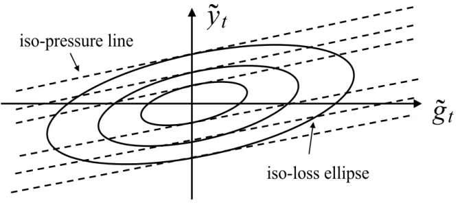
Figure 1: The Optimal Policy Mix

g

_t

y

t

iso-loss ellipse

iso-pressure line

Figure 1: The Optimal Policy Mix

deviating from the aggregate social planner’s allocation and minimising the price dispersion costs generated as the economy returns to its ecient allocation. In our sticky price/wage economy the rate of wage adjustment is driven by the extent to which households lie o their labour supply curves,

e

{w= (1 +*) ˜|w "

1(˜jw|w˜)$w˜ ln(1˜w) +zw (53)

when e{w , the forcing variable in the New Keynesian Phillips curve for wages, is positive workers are lying below their labour supply curves and are attempting to raise wages. The greater the size of {we, the faster the speed of wage adjustment. This wage adjustment, in turn aects the rate of price adjustment of rms as they attempt to return to their labour demand curves. The policy maker must therefore use their policy instruments, |w˜ and jw˜, to obtain the appropriate balance between minimising the deviation from the socal planner’s aggregate allocation and the optimal speed of price and wage adjustment. While this is an intertemporal problem, the balance between the two instruments in any given period is not. We can consider the optimal balance between the two instruments by adding a second line to the diagram in Figure 1 capturing the combinations of ˜

|w and ˜jw which generate a given level of wage pressure,{we. The slope of these ‘iso-pressure’ lines

can represent (see Figure1) the losses from deviating from the social planner’s aggregate allocation as a set of iso-loss ellipses in government spending and output gap space where the slope of a given iso-loss ellipse is given by

d˜yt d˜gt = − χ 1−α(˜gt−y˜t) (1 +ϕ)˜yt−₁₋χ_α(˜gt−y˜t)

Note that when ˜gt= 0 the slope is given by

d˜yt d˜gt = χ 1−α (1 +ϕ) +₁₋χ_α.

At any point in time the policy maker must strike a balance between minimising the losses from deviating from the aggregate social planner’s allocation and minimising the price dispersion costs generated as the economy returns to its efficient allocation. In our sticky price/wage economy the rate of wage adjustment is driven by the extent to which households lie off their labour supply curves, ˜ xt= (1 +ϕ) ˜yt− χ 1−α(˜gt−y˜t)−ω˜t−ln(1−τ˜t) +µ w t

When ˜xt, the forcing variable in the New Keynesian Phillips curve for wages, is positive workers

(20)

are lying below their labour supply curves and are attempting to raise wages. The greater the size of ˜xt, the faster the speed of wage adjustment. This wage adjustment, in turn affects the rate of

price adjustment of firms as they attempt to return to their labour demand curves. The policy maker must therefore use their policy instruments, ˜yt and ˜gt, to obtain the appropriate balance

between minimising the deviation from the social planner’s aggregate allocation and the optimal speed of price and wage adjustment. While this is an intertemporal problem, the balance between the two instruments in any given period is not. We can consider the optimal balance between the two instruments by adding a second line to the diagram in Figure 1capturing the combinations of ˜

yt and ˜gt which generate a given level of wage pressure, ˜xt. The slope of these ‘iso-pressure’ lines

are given by d˜yt d˜gt = χ 1−α (1 +ϕ) +₁₋χ_α

which is tangential to the iso-loss ellipse when ˜gt= 0. In other words, the policy maker minimises the

losses from achieving a given level of wage pressure (positive or negative) by setting the government spending gap to zero.

The positive slope of the wage pressure line is crucial to understanding why a simple notion of ’burden sharing’ is misleading. Following a positive markup shock, monetary policy will create a negative output gap by reducing private consumption. In these circumstances, it might be thought that welfare could be improved by keeping the output gap unchanged, but reducing the consumption gap by creating a negative government spending gap so that monetary and fiscal policy share the burden of controlling inflation. If the wage pressure line was horizontal, then we could move to a lower iso-loss ellipse in this way. But the wage pressure line has a positive slope: raising consumption by cutting public spending would reduce labour supply, so wage pressure would increase even if the output gap was unchanged.

The key to obtaining this result is that wage and price setters are attempting to return to labour demand and supply curves which evaluate the trade-off between consumption and leisure in the same way as the social planner. The result would not hold if the economy was distorted such that there was an endogenous wedge between the social planner’s evaluation of the marginal

(21)

rate of substitution (MRS) between consumption and leisure and the wage-setters’ evaluation of the MRS. Such an endogenous wedge could be due to, for example, habits induced by consump-tion externalities or steady-state monopolistic competiconsump-tion or tax distorconsump-tions. Suppose the wedge between private and social MRS is given by the following log-linearised function,φ(˜gt,y˜t). In this

case the slope of the iso-pressure line would be given by,

d˜yt d˜gt = χ 1−α+ ∂φ(˜gt,y˜t) ∂˜gt (1 +ϕ) +₁₋χ_α +∂φ(˜gt,˜yt) ∂y˜t

which would no longer necessarily be tangential to the iso-loss ellipse at ˜gt= 0. In other words

vari-ations in the government spending gap are only an effective policy tool (assuming the policymaker has control of the output gap through monetary policy) when there are additional distortions in the economy implying that the private and social evaluations of the MRS differ.

To make this point clearer, consider an example where the private evaluation of the elasticity of the disutility of labour, ϕ, differs from the social evaluation of this elasticity, ϕs, due to an externality. For example when ϕ <(>)ϕs _{workers are under (over)-estimating the marginal social}

cost of working. Assuming that this externality has been corrected in steady-state4, the wedge between the private and public evaluation of the marginal rate of substitution is given by,φ(˜gt,y˜t) =

(ϕs−ϕ)˜yt and the point of tangency between the iso-loss ellipse and the iso-pressure line is given

by

(1 +ϕs) y˜t ˜ gt−y˜t

= 1 +ϕ

such that ˜gt>(<)0 whenϕ >(<)ϕs. In other words when the social disutility of labour supply is

greater than workers’ private evaluation of that disutility the government spending gap is negative (rather than zero) as, in addition to stabilising the sticky-price economy in the face of shocks, the policymaker seeks to correct the household’s suboptimally high supply of labour by reducing public consumption, freeing resources for private consumption and discouraging labour supply. However, it should be noted that standard reasons for such externalities - for example, habits effects, tax

4_{A steady-state subsidy of (1}₋ κ) = (1−α+χ) ϕ−ϕs 1+ϕs₍₁₋1 )(1− 1 w)(1−τ

s₎₍₁₋_τ₎_/₍₁₋_α_{) will ensure that the} steady-state remains efficient in the presence of this additional externality.

(22)

distortions and monopolistic competition inefficiencies - do not give rise to quantitatively significant fluctuations in the government spending gap.5

Finally, we should note that the proposition applies to the government spending gap, and not to the level of government spending. As our discussion of the central planner’s problem makes clear, any shock that raises the natural level of output will also imply a matching adjustment to the optimal provision of public goods. It should also be clear that the existence of unconstrained monetary policy, enabling policy to effectively control consumption, is critical to this result. As

Gal´ı and Monacelli(2008) show, in a similar model without wage inertia, a monetary union member facing idiosyncratic shocks will be varying the government spending gap.

4 Extensions

Two questions naturally arise from this result. The first is how robust it might be to extensions to the model. While a comprehensive answer to this question is not possible in a single paper, we look at two important examples: inflation inertia and government debt. In the case of inflation inertia, we show analytically that our proposition is unchanged: the optimal government spending gap is zero. In the case of debt, we show that our analytical result no longer holds, because the optimal response to any shock is to allow a permanent change in debt, which in part will be financed by a change in government spending. However, our analysis shows that government spending is still not being used as a device for stabilising output and inflation when debt is added to the model. This helps to explain numerical results in other studies. A second question is whether the absence of a stabilisation role for government spending under optimal policy extends to tax instruments as well. A final section of the paper shows that it does not, and why there is a clear difference between tax changes and spending changes in this respect.

5

Leith et al. (2009) consider a sticky-price economy subject to ‘deep’ habits as in Ravn et al. (2006), where households do not internalise the externalities associated with their consumption decisions over individual goods. For a commonly used parameterisation this implies that steady-state consumption is 50% higher than that which would be chosen by a social planner. Despite this massive externality the use of the government spending gap as stabilisation instrument remains negligible. This is also true for tax and monopolistic competition distortions where the absolute size of the distortion is typically smaller.

(23)

4.1 Inflation Inertia

A common theme of a number of empirical studies is that the economy is subject to some degree of inflation inertia, in the sense that lagged inflation appears alongside expected inflation in the Phillips curve. A number of recent papers have examined the implications of inflation inertia for optimal monetary policy (e.g. Steinsson(2003), Sheedy (2007), Kirsanova et al. (2007)). In order to demonstrate the robustness of our key proposition to the addition of inflation persistence to the model, we assume that some price and wage setters follow backward-looking rules of thumb. The structure of our set-up is similar to Steinsson (2003). Specifically, when a firm is given the opportunity of posting a new price, we assume that rather than posting the profit maximising price (70), a proportion of those firms,ζ, follows a simple rule of thumb in resetting that price:

P_tb=P_t∗₋₁Πt−1(M Ct−1eµt−1)δ, (53)

whereP_t∗₋₁ denotes an index of the prices given by

lnP_t∗₋₁ = (1−ζ) lnP_tf₋₁+ζP_tb₋₁. (54)

andM Ct−1eµt−1 >1 captures the extent to which the price is less than marginal cost after adjusting

for the desired mark-up or, equivalently, the extent to which the typical firm lies below their labour demand curve.

Note that unlike Steinsson(2003) we specify the rule of thumb as a function of the extent to which the firm lies off its labour demand curve rather than output. The rule implies that firms posting a rule of thumb price do so by taking the optimal price from the previous period, scaling it up by last periods rate of inflation and further scaling it up to the extent that last period’s price was below its (static) profit maximising level. As Steinsson(2003)’s model involves a closed economy without government spending and with only price inertia, then labour market disequilibrium and output move together, so the two formulations are equivalent. When δ = 0 the rule of thumb reduces to that considered by Gal´ı and Gertler (1999).

(24)

Denoting the fixed share of price-setters following the rule of thumb (53) by ζ, we can derive a price inflation Phillips Curve as detailed in appendix A.5. For this we combine these rule of thumb price and wage setters with the wage and price setting described above, leading to the price Phillips-Curve πH,t=χfβEtπH,t+1+χbπH,t−1+κc( ˜mct+ ˜µt) +κb( ˜mct−1+ ˜µt−1), (55) where ˜mct+µt= ˜ωt−ln(1−τ˜s), χf ≡ _Φθ,χb≡ _Φζ,κc≡ (1−θ)[(1−ζ)(1_Φ−θβ)−θβζδ] κb≡ (1 −θ)ζδ Φ , where Φ≡θ(1 +βζ) + (1−θ)ζ.

UnlikeSteinsson(2003) where rule of thumb behaviour is restricted to price-setting, we employ a similar set-up in the labour market whereζw of wage-setters who have been given the signal to

re-set wages do so according to the rule of thumb

W_tb =W_t∗−1πtw−1 Xt−1 X δw , (56)

where lnXt≡ϕnt+wϕwt+ct+pt−ln(1−τt) +µwt. Analogous to the price setting rule,Xt−1 >1

captures the extent to which wage-setters lay below their labour supply curves in the previous period. When δw = 0, this reduces to the rule of thumb for wage setting considered byLeith and

Malley (2005).

We define ζw as the fixed share of wage-setters following (56). Appendix A.5 shows how to

obtain the wage-inflation Phillips curve

π_tw =χw_fβEtπtw+1+χwbπwt−1+κwcx˜t+κwbx˜t−1, (57)

wherext≡ϕnt+wϕwt+ct+pt−ln(1−τt) +µwt, which can be written as ˜xt= ϕ+₁₋1_γ ˜ yt− γ 1−γg˜t−ω˜ −ln(1−τ˜t) + ˜µwt, and χwf ≡ θw Φw, χwb ≡ ζw Φw, κwc ≡ (1−θw)(1−ζw) Φw 1−θwβ 1+ϕw − ζwδwθwβ 1−ζw , κw_b ≡ (1−θw)ζwδw Φw .

The rule of thumb behaviour adds price and wage inflation persistence to the model, while the presence of the activity variables in each rule of thumb add additional dynamics in the forcing

(25)

variables driving price and wage inflation. However, the relationship between the government spending gap and output gap in the lagged forcing term driving wage inflation is identical to the relationship in the current period forcing term (i.e. these gaps only appear in ˜xt and ˜xt−1) and

equivalently in the term that would occur if there were no rule of thumb price setters. This will be crucial below.

To consider the impact this generalisation has on optimal policy we must rederive the objective function, since the evolution of price dispersion (which underpins the presence of the quadratic term in inflation) will be affected by the rule of thumb behaviour. UsingSteinsson(2003)6_{, we can}

show that the objective function can be written as −(1−α₂+χ)P∞

t=0βtLt+t.i.p.+okak3 with the

per period loss function defined as

Lt = λπ 2 H,t+ w ˜ λw (π_tw)2+ (1 +ϕ)˜y2+ χ 1−α(˜gt−y˜t) 2 (58) + λ ζ (1−ζ)θ[πt−(πt−1+ (1−θ)δ( ˜mct−1+ ˜µt−1)] 2 +w ˜ λw ζw (1−ζw)θw [πw_t −(π_tw−1+ (1−θw)δwx˜t−1)]2. (59)

Rule of thumb price and wage setters introduce the last two terms in this per period loss function. While this greatly complicates the optimal policy trade-offs between inflation, output and the change in inflation, as discussed in Steinsson (2003), a key point to note in the current context is that the additional terms in the government spending and output gaps are constrained to be in the form governed by ˜xt−1, which is the same as the forcing variable in the NKPC.

Given the loss function (58) the Lagrangian is

(26)

Lt=− 1 2 ∞ X t=0 βt[ λπ 2 H,t+ w ˜ λw (π_tw)2+ (1 +ϕ)˜y2+ χ 1−α(˜gt−y˜t) 2 + λ ω (1−ω)θ[πt−(πt−1+ (1−θ)δmc˜ t−1)] 2 + w ˜ λw ωw (1−ωw)θw [π_tw−(πw_t−1+ (1−θw)δwx˜t−1)]2 −2Λpc_t (χfβEtπH,t+1+χbπH,t−1+κc( ˜mct+ ˜µt) +κb( ˜mct−1+ ˜µt−1)−πH,t) −2Λpcw_t (χw_fβEtπtw+1+χwbπwt−1+κwcx˜t+κbwx˜t−1−πwt) −2Λw_t (˜ωt−1−πt+πwt −∆ωtn−ω˜t)]. (60)

In order to reconsider the impact of these extensions on our key result we need to undertake the same optimisation we did previously. Here we focus on the first-order conditions for output and government spending

−(1 +ϕ)˜yt+ χ 1−α(˜gt−y˜t) + ϕ+ 1 1−γ (κw_cΛpcw_t +κw_bβΛpcw_t₊₁) = 0 (61) − χ 1−α(˜gt−y˜t)− χ 1−α(κ w cΛ pcw t +κwbβΛ pcw t+1) = 0. (62)

We can combine these optimality conditions (together with γ = ₁₋_αχ₊_χ), and once again we obtain

˜ gt= 0.

Thus, in a richer model with persistence in wage and price inflation and where the lags in the forcing variables influence wage and/or price inflation, our key proposition re-emerges unscathed. Despite the fact that monetary policy will seek to influence the path of the output gap in the face of shocks, under the optimal commitment policy, there is no desire to deviate from a government spending gap of zero.

We can now return to an issue we considered earlier, the definition of the activity variable in the rule of thumb price and wage setting behaviour. If we had adopted a definition of the activity variable which didn’t reflect the extent of wage and/or price disequilibrium then there

(27)

would be scope for the policymaker to use the government spending gap to exploit this difference in price/wage setting.7 However, as the above analysis shows, this use of government spending as a stabilisation tool would depend entirely on the ad-hoc use of an activity variable unrelated to profit/utility maximising behaviour in rule of thumb price setting behaviour, rather than the existence of rule of thumb price setters per se.

4.2 Government Debt

In this subsection we consider the impact of introducing government debt into our analysis of policy within a small open economy.8 Until now we have assumed that there was a lump-sum tax instrument which was utilised to balance the budget whenever other fiscal instruments were used in a stabilisation role. In this section, any inconsistency between government tax revenues and spending will affect government debt. Policy must then ensure that any relevant government budget constraint is satisfied. Lump-sum taxes remain, but only to finance the steady-state subsidy; they cannot be varied out of steady state.

The flow budget constraint for our economy has the form

Bt=Rt−1Bt−1+PtGt−PtYtτts−WtNtτt, (63)

where Bt is government debt. Rewriting this in real terms and in a form consistent with the

definitions of the tax rates in terms of gaps we obtain Bt Pt =Rt−1 Pt−1 Pt Bt−1 Pt−1 −Yt+Gt+Yt(1−τts) + Wt Pt Nt(1−τt)− Wt Pt Nt. (64) 7

SeeStehn and Vines(2007) for example.

8_In _{Leith and Wren-Lewis} ₍₂₀₀₅_{), we consider the significance of adding debt to New Keynesian models of} monetary policy more fully.

(28)

This can be log-linearised as bt = Rbt−1+R(rt−1−πt) + G B lnGt+ (1−τs)Y B ln(1−τ s t) −τ s_Y B yt+ (1−τ)rwN B ln(1−τt)− τ rwN B/P (rwt+nt) −RlnB−R(r)−G B lnG− (1−τs)Y b ln(1−τt) −τ s_Y B Y i +(1−τ)rwN B ln(1−τ)− τ rwN B (rw+n),

where bt = ln(B_Pt_t) and B = (B/P).Rewriting in gap form, using the production function to first

order, ˜yt= ˜nt, this can be written as

˜_b_t ₌ _R˜_b_t₋₁₊_R(˜_r_t₋₁₋_π_t_{) +}G bg˜t+ (1−τs_)y b ln(1−τ˜ s t) −(τ s_Y B + τ rwN B )˜yt+ (1−τ)rwN B ln(1−˜τt)− τ rwN B (rw˜t)

The welfare function remains unchanged, so the Lagrangian of our policy problem has this additional constraint with lagrange multiplier Λb_t added to it. As the budget constraint also involves the real interest rate gap, we also need to reintroduce the IS curve constraint, with multiplier Λis_t

L_t=−1 2 ∞ X t=0 βt[ λπ 2 H,t+ w ˜ λw (π_tw)2+ (1 +ϕ)˜y2+ χ 1−α(˜gt−y˜t) 2 −2Λpc_t (βEtπH,t+1+λ(˜ωt−ln(1−τ˜ts) + ˜µt)−πH,t) −2Λpcw_t (βEtπtw+1+ ˜λw ϕ+ 1 1−γ ˜ yt− γ 1−γ˜gt−ω˜t−ln(1−τ˜t) + ˜µ w t −πw_t) −2Λw_t (˜ωt−1−πt+πwt −∆ωtn−ω˜t) −2Λis_t (˜yt−γ˜gt−E{˜yt+1−γg˜t+1+ (1 +γ)πt+1}+ (1−γ)˜rt) −2Λb_t(˜bt−Rb˜t−1−R(˜rt−1−πt)−bg˜gt−bτsln(1−τ˜_ts) +byy˜t−bτln(1−τ˜t) +brwrw˜t)], (65) where bg = G_B, bτs = (1−τ s₎_Y B ,by = τ rwN B + τ rwN B ,bτ = (1−τ)rwN B , and brw = τ rwN

(29)

condition under commitment for the interest rate is given by

(1−γ)Λy_t −EtΛbt+1 = 0. (66)

Here monetary policy must now take account of its impact on the government’s finances. The first-order condition for debt is

Λb_t−EtΛbt+1= 0,

which implies that, E0Λbt = Λb ∀t. In other words, following a shock policy must ensure that the

‘cost’ of the government’s budget constraint is constant. This is the basis of the random walk result of Schmitt-Groh´e and Uribe(2004). The first-order condition for the government spending gap is

− χ 1−α(˜gt−y˜t)−˜λw γ 1−γΛ pcw t −γΛ y t +β−1γΛ y t−1−bgΛ b t = 0

and that of the output gap

−(1 +ϕ)˜yt+ χ 1−α(˜gt−y˜t)−λ˜w ϕ+ 1 1−γ Λpcw_t + Λy_t −β−1Λy_t₋₁+byΛbt = 0.

Fort >0 these can be combined as

−(1 +ϕ) ˜gt+φΛbt = 0, (67)

whereφ=−ϕ+1−₁₋α+_αχ1−_χαbg+ϕ(1−β−1) +by.9 Equation (67) implies that the need to finance

the government’s budget constraint forces the policymaker to adjust the government spending gap. However, given that Λb_t is constant in the absence of new information, this condition implies that there will be a permanent deviation of the government spending gap from zero following a shock with fiscal consequences. In other words, beyond the need to ensure the intertemporal budget

9 _{Note that policy instruments may be used to exploit the fact that expectations are taken as given in the initial} period as the policymaker seeks to reduce the size of the cost of satisfying the government budget constraint, Λbt through such devices as inflation surprises when debt is nominal - see Leith and Wren-Lewis (2008). However, from that point on, in the absence of new information, the government spending gap will be constant and will not play any countercyclical role.

(30)

constraint is satisfied, there is no attempt to further adjust the government spending gap as a means of stabilising the economy. Here the government spending gap is being used to stabilise debt, and not to stabilise output and inflation following shocks.

The reason why the government spending gap is used to finance the new steady-state level of debt following shocks with fiscal consequences mirrors the reason why it is not used as a stabilisation device more generally. Whereas the stabilisation problem required the policymaker to achieve the biggest correction to inflationary pressure from a given welfare cost of efficiency gaps, the financing of government debt requires the greatest fiscal correction without generating inflationary pressure. Accordingly, an appropriate combination of higher taxation and lower government spending can service higher debt (without generating inflation) more effectively than utilising the tax instrument alone.

This result may help us understand some results in the literature. Kirsanova and Wren-Lewis

(2007), examine a model which is very similar to a closed economy version of our model with debt. Monetary policy is optimal (operating under commitment), and fiscal policy is either chosen optimally or is restricted to a simple rule whose only argument is the stock of government debt. This simple rule is described as ‘fiscal feedback’, and cuts the government spending gap relative to steady state if debt rises above steady state. This rule precludes any demand management role for government spending. The focus of the paper is on the implications of different speeds of fiscal feedback for both monetary policy and the economy as a whole. One result they obtain is that feedback that just stabilises debt comes very close to duplicating the optimal policy for debt, which is that steady state debt follows a random walk. The difference in social welfare following a standard cost-push shock is of the order of 0.002% of steady state consumption. Thus an optimal simple fiscal rule which prevents any countercyclical fiscal role is a restriction with negligible welfare costs, and therefore by implication any additional fiscal demand management would at best make a negligible contribution to social welfare. The reason for this numerical result becomes apparent given the analysis in this section.10

The reason why the government spending gap is used to finance the new steady-state level of

10

(31)

debt following shocks with fiscal consequences mirrors the reason why it is not used as a stabilisation device more generally.Whereas the stabilisation problem required the policymaker to achieve the biggest correction to inflationary pressure from a given welfare cost of efficiency gaps, the financing of government debt requires the greatest fiscal correction without generating inflationary pressure. Accordingly, an appropriate combination of higher taxation and lower government spending can service higher debt (without generating inflation) more effectively than utilising the tax instrument alone.

Schmitt-Groh´e and Uribe (2007) compares alternative fiscal and monetary policy rules with a Ramsey policy, using a fairly elaborate model with capital, money and debt, but one which can be viewed as an extension of the closed economy version of our baseline model. Although their fiscal rules involve income taxes rather than government spending, they are restricted to feedback on government debt alone, and so they exclude any direct countercyclical role.11 They also find that, when their monetary policy rules are suitably aggressive, these two rules combined come close to replicating the Ramsey policy. The cost of following simple rules for both monetary and fiscal policy compared to the Ramsey policy can be as low as 0.003% of steady state consumption. By implication, the cost of excluding any countercyclical role for fiscal policy must be at least as small as this number.

Our analysis suggests that adding government debt to our analysis does not alter our conclusions in a material way. However, it is important to note that here, at least, the assumption that policy can be time inconsistent is important for the welfare consequences of shocks. Leith and Wren-Lewis

(2007b) show that under discretion, steady state debt no longer follows a random walk. Instead, fiscal or monetary instruments must be used to bring debt back to its original, pre-shock level, on the assumption that this level was efficient. Taking the example of a technology shock in our baseline model, Leith and Wren-Lewis (2007a) show that allowing for debt adds around 13% to welfare costs under discretion, compared to 2.4% under commitment.

11_{We argue below that taxes, rather than government spending, can play a complementary role to monetary policy} when there are cost-push shocks or wage inertia. The models inSchmitt-Groh´e and Uribe(2007) do not include either distortion.

(32)

4.3 Taxes

So far we have focused on government spending as an instrument of fiscal policy. In our view this comes closest to representing fiscal policy as a demand management tool, which is the theme of this paper. We have shown that there is no role for government spending as part of a countercyclical policy if monetary policy is optimal and unconstrained. However, it would be quite incorrect to infer from this that fiscal policy in general has no short-term stabilisation role. In our analysis so far, we assumed both tax rates were fixed. Suppose instead that we allowed them to vary in an optimal manner. Using the Lagrangian (40) from our baseline model, we would obtain two additional first order conditions. For the production tax gap, ln(1−˜τs), it is

λλπ_t = 0. (68)

Thus the NKPC for prices ceases to be a constraint on maximising welfare, as production tax changes can offset the impact of any other variables driving price inflation. In particular production taxes that can vary period by period can eliminate completely any mark-up shocks.

Similarly, the condition for income taxes is given by

˜ λwλπ

w

t = 0. (69)

Leith and Wren-Lewis(2007a) show that a combination of production and income taxes, combined with an optimal monetary policy, can completely eliminate the impact of technology shocks on social welfare when we have sticky wages.

These two conditions show that tax changes work in distinctly complementary ways to monetary policy. In the first case, production taxes represent a distortionary tax that works on the same margin as a distortionary shock, so we can use one distortion to offset another. This point would hold in a flexible price world. In the second case, income taxes help offset the impact of nominal wage rigidity. As we noted above, monetary policy alone cannot eliminate the impact of technology shocks when both nominal wage and price inertia are present. So here, changes in taxes can clearly

(33)

assist monetary policy in its stabilising role. This result may be an example of a more general point. There may be other examples where different degrees of nominal inertia among different agents or sectors can lead to distortionary movements in relative prices, and where there exists a tax instruments that may be able to offset these relative price changes. One example might be taxes on domestic sales and differences in inertia between traded and non-traded goods.

Why do tax changes appear to be a useful complement to monetary policy in these situations when changes in government spending were not? The key point is that taxes are useful because they help change relative prices in a way that monetary policy cannot. In contrast, the stabilisation role for government spending is in changing demand, and here it can do nothing to assist an unconstrained optimal monetary policy.

5 Conclusion

As recent events have shown, there remain occasions in which policymakers wish to supplement monetary policy with fiscal action to control the business cycle, but macroeconomists appear divided on whether and when such action is warranted. This paper attempts to clarify that debate, asking whether fiscal action in the form of changes to the government spending gap can assist a fully optimal and unconstrained monetary policy under commitment.

In our baseline model, which includes both nominal wage and price rigidity, we show that optimal fiscal policy should play no role in helping to stabilise output or inflation, whether shocks come from technology, preferences or price mark-ups, and whether the economy is open or closed. The optimal government spending gap is always zero. In this context, monetary policy is indeed all we need. This is despite the fact that, in the presence of wage as well as price inertia, or for cost-push shocks under just price inertia, optimal monetary policy is unable to eliminate the welfare costs of such shocks.

These analytic results are robust to supplementing the model with forms of inflation inertia. When we assume lump sum taxes are no longer available to prevent shocks and policy from changing government debt, the optimal government spending gap is no longer zero. However we show

(34)

analytically that the government spending gap moves in a way which optimally finances a new level of government debt, and so it continues not to play any stabilisation role. This helps explain numerical results in two recent papers12, where fiscal policy that is constrained to follow simple feedback rules from debt can come close to replicating the unconstrained social optimum.

Finally, we use our baseline model to show that these results apply only to government spending as an instrument, representing a demand management role for fiscal policy. We note situations in which variations in tax rates, by changing the relative price of leisure, can play a complementary role to monetary policy. It is therefore incorrect to conclude that fiscal policy in all its forms can play no useful role in short term stabilisation. We should also stress that our analysis of the demand management role of fiscal policy is confined to cases where monetary policy is both optimal and unconstrained: interest rates can be costlessly adjusted to influence consumption and there are, for example, no problems with interest rates hitting a lower bound.

A

Appendix

A.1 Price Setting

Facing the objective function (19), the optimal price set by firms that are able to reset prices in period tis PH,t= −1 EtP∞s=0(θ)sQt,t+s h (1−_κ)Wt+s Pt+sP H,t+s Yt+s At+s i EtP∞s=0(θ)sQt,t+s h (1−τr t+s)P −1 t+sPH,t +sYt+s i. (70) In equilibrium βs Ct Ct+s Pt Pt+s

= Qt,t+s, so that the expression for the optimal price can be

re-written as PH,t= −1 EtP∞_s₌₀(θβ)s_C_t₊C_st_{P t}Pt₊_s h (1−_κ)Wt+s Pt+sP H,t+s Yt+s At+s i Et P∞ s=0(θβ)sCt+CstP tPt+s h (1−τ_tr₊_s)P_t−₊1_sP_H,t ₊_sYt+s i

Allowing the mark-up to be time varying due to mark-up shocks, this can be log-linearised as

p_H,t= (1−θβ)Et ∞ X s=0 (θwβ)s −at+s+wt+s−ln(1−τtr+s)−v+µt !

(35)

wherep_H,t is the log of the optimal price set by those firms that were able to set price in period t and µtis a shock to the desired mark-up. Quasi-differencing this expression yields,

1 1−θβpH,t= 1 1−θβθβEtpH,t+1−at+wt−ln(1−τ r t)−v+µt

Domestic prices evolve according toPH,t = h (1−θ)P1_H,t−+θP_H,t1−₋₁ i 1 1− , or log-linearised pH,t= (1−θ)pH,t+θpH,t−1. (71)

Solving for p_H,t and substituting into the expression for quasi-differenced optimal price yields

1 1−θβ pH,t 1−θ− θpH,t−1 1−θ = 1 1−θβθβ EtpH,t+1 1−θ − θpH,t 1−θ −at+wt−ln(1−τtr)−v+µt

This can be solved as (20).

A.2 Wage Setting

Recall the optimal wage set by those households that are able to re-set wages in period t,

W(k)−1−ϕw t = Et P∞_s₌₀(θw)s Qt,t+sWt+wsNt+s(1−τt+s) Et P∞ s=0(θw)s h Qt,t+sµwWt+w(1+s ϕ)N 1+ϕ t+s Ct+sPt+s i (72)

Note that in equilibrium βs Ct

Ct+s

Pt

Pt+s

= Qt,t+s. Accordingly the expression for the optimal

re-set wage is given by

W−_t1−ϕw = Et P∞ s=0(θwβ)s Ww t+sNt+s(1−τt+s)Ct−+1sP −1 t+s Et P∞ s=0(θwβ)s h µwWt+w(1+s ϕ)N 1+ϕ t+s i (73)

After introducing a time varying desired mark-up,µw_t, this expression can be log-linearised as

1 +ϕw 1−θwβ wt=Et ∞ X s=0 (θwβ)s[ϕnt+s+wϕwt+s+ct+s+pt+s−ln(1−τt+s) +µwt] ! (74)

(36)

Quasi-differencing this expression yields 1 +ϕw 1−θwβ wt= 1 +ϕw 1−θwβ awβEtwt+1+ϕnt+s+wϕwt+s+ct+s+pt+s−ln(1−τt+s) +µwt (75)

The wage index evolves according to the law of motion Wt= h (1−θw)W (1−w) t +θwWt1−−1w i₁₋1_w , which log-linearised gives

wt= (1−θw)wt+θwwt−1 (76)

(74) and (76) can be solved for wage inflation to obtain (9).

A.3 Derivation of Loss Function

The measure of social welfare is obtained as a second-order approximation to the utility of the representative agents (1). Note the following general result relating to second order approximations,

Xt−X Xt = ˜xt+ 1 2x˜ 2 t+okak 3 (77)

where okak3 represents terms that are of order higher than 3 in the bound kak on the amplitude of the relevant shocks.

The term in consumption can be written as

˜

ct=α˜c∗t + (1−α)(˜yt−g˜t). (78)

For simplicity, we can take a log-transformation of (21),

ln(Yt−Gt) =yt+ ln(1−

Gt

Yt

) =yt−ht, (79)

whereht≡ −ln(1−G_Y_tt). We can then work in terms ofht and use the approximation

˜ ht=

χ

(37)

to translate the derivation back into familiar terms in government spending and output. The term in government spending can be approximated to second order as

lnGt = ln(

Gt

Yt

) + ˜yt+t.i.p.= ln(1−exp(−ht)) + ˜y+t.i.p.

= 1−γ γ h˜t− 1 2 1−γ γ2 ˜h 2 t+ ˜yt+t.i.p.+o kak3

whereγ=G/Y. We can then write, using (29),

χlnGt= (1−α)˜ht− 1 2 1−α γ ˜h 2 t +χ˜yt+t.i.p.+okak3. (81)

Approximating the labour-supply term of an individual household k to second-order and then integrating over all households kwe obtain

Z 1 0 Nt(k)1+ϕ 1 +ϕ dk= (Nn)1+ϕ 1 +ϕ + (N n₎1+ϕ Z 1 0 ˜ nt(k)dk+ 1 2(1 +ϕ) Z 1 0 ˜ nt(k)2dk +okak3 (82)

The linear term in labour supply can be re-expressed as follows, using (84)-(86).

Z 1 0 ˜ nt(k) dk= ˜nt+w 1−w 2 vark[wt(k) 2_]. ₍₈₃₎

To obtain this use the demand for labour (7) and take logs so that

Z 1 0 ˜ nt(k) dk= ˜nt+ Z 1 0 ln Wt(k) Wt −w dk. (84)

Lettingw_bt(k) =w(k)−wt we find that

Wt(k) Wt 1−w = exp[(1−w)wbt(k)] = 1 + (1−w)wbH,t(i) + (1−w)2 2 (wbH,t(k)) 2 +okak3. (85)

From the definition ofWt we have 1 = R1

0

_W_t(_k₎ Wt

1−w

(38)

expres-sion acrossk the expression simplifies to, Ek[wbt(k] = w−1 2 Ek[wbt(k) 2_{] =} w−1 2 vark[wt(k) 2_]. ₍₈₆₎ ˜

nt, as detailed i.a. inGal´ı(2008), can be expressed as

˜ nt = y˜t+ ln[ Z 1 0 (PH,t(i) PH,t )− di] (87) = y˜t+

2vari[pH,t(i)] +okak

3

(88)

From the definition of the variance we also know that

Z 1 0 (ñt(k))2dk=vark{ñt(k)}+ ( Z 1 0 (ñt(k))dk)2, (89)

where vark[˜nt(k)] = 2wvark[wt(k)]. Using (83) and (89) in (82) and combing the latter with (78)

and (81) we obtain ∞ X t=0 −1−α+χ 2 β t 1−α χ ˜ h2_t + (1 +ϕ)˜y_t2+ varl[pt(l)] +w(1 +ϕw)vark[wt(k)2] +tip+okak3 (90)

Woodford (2003), chapter 6, shows that under the assumption of Calvo-pricing

X βtvarl[pi,t(l)] = 1 λ X βtπ2_i,t. (91)

Given the Calvo price-setting rules in wage-setting this also implies

∞ X t=0 βtvark[wt(k)] = 1 λw ∞ X t=0 βt(π_tw)2+t.i.p+okak3. (92)

Using (91) and (92) as well as (80) in connection with (29) we obtain (38) and (39).

A.4 Rule of Thumb in Price Setting

When is monetary policy all we need?