Rent’s Rule and Parallel Programs:
Characterizing Network Traffic Behavior
Wim Heirman, Joni Dambre, Dirk Stroobandt, Jan Van Campenhout
Ghent University, ELIS Sint-Pietersnieuwstraat 41
9000 Gent, Belgium
[email protected]
ABSTRACT
In VLSI systems, Rent’s rule characterizes the locality of interconnect between different subsystems, and allows an ef-ficient layout of the circuit on a chip. With rising complex-ities of both hardware and software, Systems-on-Chip are converging to multiprocessor architectures connected by a Network-on-Chip. Here, packets are routed instead of wires, and threads of a parallel program are distributed among pro-cessors. Still, Rent’s rule remains applicable, as it can now be used to describe the locality of network traffic. In this paper, we analyze network traffic on an on-chip network and observe the power-law relation between the size of clusters of network nodes and their external bandwidths. We then use the same techniques to study the time-varying behav-ior of the application, and derive the implications for future on-chip networks.
Categories and Subject Descriptors
C.1.4 [Processor Architectures]: Parallel Architectures—
Distributed architectures
General Terms
Algorithms, Measurement, Performance
Keywords
Rent’s rule, locality, characterization, network-on-chip, net-work traffic behavior
1. INTRODUCTION
In 1971, Landman and Russo described the relation be-tween the number of terminals (T) at the boundaries of an electronic circuit and the number of internal compo-nents (G), such as logic gates or standard cells [6]. This remarkable trend was discovered earlier by E. F. Rent, an IBM employee, who studied this relation on IBM’s inte-grated circuit designs. The same trend can be found on
Permission to make digital or hard copies of all or part of this work for personal or classroom use is granted without fee provided that copies are not made or distributed for profit or commercial advantage and that copies bear this notice and the full citation on the first page. To copy otherwise, to republish, to post on servers or to redistribute to lists, requires prior specific permission and/or a fee.
SLIP’08,April 5–6, 2008, Newcastle, United Kingdom. Copyright 2008 ACM 978-1-59593-918-0/08/04 ...$5.00.
the parts of a hierarchical partitioning (with minimal inter-partition communication) of a single circuit. Over a wide range of (sub)circuit sizes, this relation follows a power law:
T =tGp
Christie and Stroobandt later theoretically derived this pre-viously empirical rule for homogeneous systems [1]. They point out the meaning of the parameterp, the “Rent expo-nent”: smaller values ofpcorrespond to a larger fraction of local interconnects.
While VLSI systems steadily increased in size, following Moore’s law, Rent’s rule remained applicable over a wide range, from small circuits of just a few tens of gates up to multi-million gate designs. Nowadays, ad-hoc global wiring structures are being replaced by more modular interconnects such as Networks-on-Chip (NoCs), as predicted by Dally and Towles in [2]. Their philosophy is toroute packets, not wires: a generic communication structure, such as a mesh, connects all entities on a chip. Communication between specific en-tities is no longer done by connecting them directly using a dedicated set of wires, but rather by sending packets, which are routed through the network to their destination.
One can therefore ask the question: is there an equivalent of Rent’s rule for communication that does not use global wires, but a packetized network? This indeed turns out to be the case. Following Greenfield et. al. [4], we define
a bandwidthbased alternative to Rent’s rule, in which the
bandwidth (B), sent and received by a cluster of network nodes, is dependent on its size (number of nodes,N):
B=bNp (1)
Note that, when N = 1, this equation yieldsB =b. The parameter bis thus the average bandwidth per node. The exponent pwill again be dependent on communication lo-cality: smaller values ofpwill correspond to more localized communication. This will have an influence on the mapping of functional blocks to network nodes, similar as to how placement is affected in traditional VLSI design.
In [4], the implications of localized network traffic on NoC design was studied, assuming that network traffic follows Rent’s rule. In this paper, we will investigate whether this is indeed the case. Therefore, we simulate the execution of a parallel benchmark program on a network of up to 64 pro-cessors. This illustrates the case of a Chip Multi-Processor (CMP) connected by a NoC. We estimate the Rent expo-nent by hierarchically partitioning the network nodes and correlating the bandwidth sent and received by each result-ing cluster with its size. It turns out that this relationship
does follow a power law, with a Rent exponent of 0.55–0.74, depending on the application and the total network size. This proves that communication is indeed localized.
We also investigate network traffic behavior through time, by slicing up the program execution into separate intervals. We partition the network and estimate the Rent exponent for each time interval. By comparing the partitionings made in different intervals, we find that, for some benchmarks, the behavior can change quite radically through time. Both changes in traffic locality, and in partitioning are found. This last observation would implicate that different place-ments are needed through time, suggesting that, for some benchmarks, a single placement of program threads on net-work nodes can only be optimal during some time intervals, while being sub-optimal during other periods. This shows that solutions like dynamic thread movement or reconfig-urable networks are indeed necessary.
The remainder of this paper is structured as follows. Sec-tion 2 describes our simulaSec-tion platform, how we estimated Rent exponents, and defines the various metrics that were used throughout this work. In Section 3 we show estimated Rent exponents and use them to determine communication locality in the different benchmark applications. Section 4 looks at how network traffic, and its locality, vary through time. We analyze the effect of changing traffic patterns on node placement in Section 5. Finally, Section 6 provides some insights into how this work can be used in NoC design and Section 7 summarizes our conclusions.
2. METHODOLOGY
2.1 Simulation platform
Our simulation platform uses the commercially available Simics simulator [7]. It models a multiprocessing architec-ture with 16, 32 or 64 processors. Each processor, with its cache memories and a part of main memory, has a network interface. This structure forms onenetwork node. A shared memory paradigm is used, so main memory on all nodes is viewed as one global address space, accessible by all proces-sors. When a processor makes a memory access to a data word that is stored on a different node, this results in net-work traffic. As opposed to a machine using message pass-ing, in our case not only application data will pass through the network but also operating system data, synchronization variables and program code. This will have an effect on the communication patterns observed. More details about our simulation platform are described in [5].
The processors run one of the parallel applications from the SPLASH-2 benchmark suite [10], which consists of a number of scientific and technical kernels and programs that represent a typical workload of large shared-memory multi-processing machines. The programs are partitioned into
threads, each is run by one processor. For each of the
bench-marks, the execution is simulated on three network sizes (16, 32, and 64 nodes). From all simulations, a trace (timestamp, source, destination and size of each packet) is collected of all network traffic. The benchmarks, and the input sizes that were used, can be found in Table 1. For some of the benchmarks we added a *scale variant in which the size of the data set is scaled linearly with the number of pro-cessors (because the fft benchmark performs a 2-D FFT transformation, its input set has to change in multiples of four which is why we did not runfftscale on a 32-node
Benchmark Input size
barnes 8192 particles cholesky tk15.O cholesky29 tk29.O fft 256K points fft4M 4M points fftscale 256K / - / 1M points lu 512×512 matrix luscale 5122 / 10242 / 20482 matrix ocean.cont 258×258 ocean ocean.contscale 2582 / 5142 / 10262 ocean
radix 1M integers, 1024 radix
radixscale 1M / 2M / 4M integers, 1024 radix
water.sp 512 molecules
Table 1: SPLASH-2 benchmarks and input sizes
that were used in this study. When multiple
in-put sizes are given, they are for 16, 32 and 64-node networks respectively
network). While results for larger networks would be inter-esting, doing these simulations with the current platform is not feasible in practice. A 64 processor simulation of one benchmark execution can already take several days.
2.2 Estimating the Rent exponent
For each traffic trace, we do the following analysis. First, a traffic matrix is constructed. This matrix gives, for each node pair, the total amount of communication (measured in bytes) with one of the nodes as the source and the other node as destination. The communication in the system can also be modeled as a graph, with all nodes as the vertices and the bandwidth between corresponding node pairs, taken from the traffic matrix, as weights on the edges. Since most nodes tend to communicate with all other nodes, this graph is usually fully connected.
We do a top-down, min-cut partitioning of the commu-nication graph using the hMETIS partitioning tool [8]. In each step we divide the partition into two roughly equal parts1. For each partition, we record the number of nodes it
contains, and theexternalbandwidth (i.e., the sum of com-munication between all node pairs where one node of the pair is in the partition and the other node is not). This gives us a list of (number of nodes, bandwidth) or (N, B) pairs.
On all (N, B) pairs, we do a least-squares fit of the func-tion B = bNp, determining the band pparameters. The
weight of each (N, B) data point is such that each hierarchi-cal partitioning level has an equal weight on the total error, i.e., we compensate for the fact that each lower level will have twice the number of partitions.
2.3 Temporal behavior
To study the temporal behavior of the network traffic, we divide the traffic trace into intervals of equal length. On each interval, the same analysis is done as before to estimate the Rent exponent and the average node bandwidth. We then plot the Rent exponentpand the bandwidthbthrough time.
1We used hMETIS version 2.0pre1, with the default
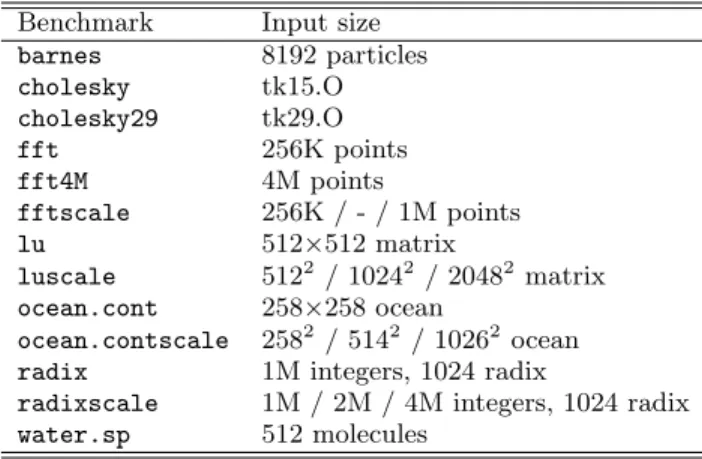
10 100 1000 1 2 4 8 Bandwidth (MB/s) Number of nodes cholesky29, 16 nodes p = 0.65 b = 68.71 100 1000 10000 1 2 4 8 16 Bandwidth (MB/s) Number of nodes ocean.cont, 32 nodes p = 0.73 b = 298.72 100 1000 10000 1 2 4 8 16 32 Bandwidth (MB/s) Number of nodes radix, 64 nodes p = 0.71 b = 329.27
Figure 1: Distribution of node count and bandwidth for all hierarchical partitions, with network sizes ranging from 16 to 64 processors executing thecholesky, ocean.contorradixbenchmark application. Rent exponent
pand average node bandwidthb(in MB/s) are fitted to this distribution using the power law B=bNp
This allows us to study the temporal variability of traffic locality and bandwidth requirements.
When mapping program threads to network nodes, the partitioning made in the previous section can be used advan-tageously. To investigate how this partitioning, and the re-sulting node placement, change through time, we construct an interval similarity function. This function should be a measure for how well the partitionings of two distinct inter-vals agree. Since the bandwidth requirements have a large impact on performance – when two nodes communicate only sparsely, moving them around between partitions will have little influence – the communication intensity should there-fore have a large impact on the similarity metric.
Non-local communication has the largest influence, so we only look at the topmost two levels of partitioning. Defining partA as the partitioning made for interval A, and trafficB
as the traffic matrix in intervalB, we derive the similarity metric as follows. From partA, the topmost two levels of the
partitioning are selected as part2
A, this gives us six clusters
of nodes. We then compute the total traffic that crosses all cluster boundaries in part2
A, assuming the traffic pattern is
trafficB, this isT(partA,trafficB) or justTA,B. WhenA= B, thenTA,B is the sum of six of the same external cluster bandwidths that were measured in section 2.2. ForA6=B, it provides a measurement of how good the partitioning made in interval A is, when the traffic pattern changes to that observed in intervalB.
To construct a bandwidth-independent metric that can be compared across intervals, we compute:
sim0
A,B= TB,B TA,B
Assuming the min-cut partitioning is done optimally,TB,B≤
TA,B so sim0
A,B ≤1. To make the metric symmetrical, we
define our similarity metric between intervalsAandB as: simA,B= TA,A+TB,B
TB,A+TA,B
which again will be in the range 0..1. Note that, when the bandwidth in intervalA is much larger than that in inter-valB, theT∗,Aterms will dominate such that:
simA,B' TA,A TB,A
In this case, only the deviation of the partitioning inB for trafficAwill be of importance, the fact that partitioningA
may be suboptimal for traffic B is much less relevant since the low-intensity interval B will not have a big influence on network performance. This is reflected in our similarity metric simA,B.
Finally, we asses the optimality of a single placement for the whole program. We assume this placement will be de-rived from a given partitioningP. We define the suitability of the placement derived fromP for the traffic measured in intervalAas:
suitP,A=T(partA,trafficA) T(P,trafficA)
We average this over the course of the program, considering that intervals with less traffic are less important, by com-puting: suitP = P AT(partA,trafficA) P AT(P,trafficA)
3. NETWORK TRAFFIC LOCALITY
As detailed in Section 2, we simulate the execution of all benchmarks on networks of up to 64 processor nodes. On the resulting traffic traces, traffic matrices are computed which are then used to do a top-down min-cut partitioning of the nodes. We record the size and external bandwidth of each cluster. In Figure 1, the distribution of bandwidth versus node count is plotted for all partitions on network sizes of 16, 32 and 64 processors. On a log-log scale, the power law relation is clearly visible. Still, between individual nodes, there can be a large variation.With thecholesky29benchmark, one node has a much higher than average bandwidth. For all cluster sizes, the cluster containing this node clearly sticks out. This would mean that this one node is heavily communicating with most other nodes. Indeed, when analyzing the benchmark’s be-havior we can find that a very important and high-traffic data structure, a task queue from which all processors re-trieve work items and insert new work, is located on this node. This causes communication between the memory on this node and the processors on all other nodes. Other benchmarks, such as radix, have much more uniform com-munication bandwidths.
The Rent exponentpand average node bandwidthbare fitted to the distributions of Figure 1 for all benchmarks. The resulting Rent exponents are shown in Table 2. We find thatpvaries between 0.55 and 0.74. Its exact value depends
Benchmark Rent exponent
16 nodes 32 nodes 64 nodes
barnes 0.61 0.69 0.72 cholesky 0.61 0.69 0.67 cholesky29 0.65 0.69 0.71 fft 0.59 0.71 0.74 fft4M 0.62 0.59 0.66 fftscale 0.59 0.72 lu 0.61 0.71 0.72 luscale 0.61 0.71 0.73 ocean.cont 0.55 0.73 0.74 ocean.contscale 0.55 0.70 0.67 radix 0.56 0.69 0.71 radixscale 0.57 0.69 0.70 water.nsq 0.61 0.71 0.71 water.sp 0.61 0.70 0.74
Table 2: Estimated Rent exponents for all bench-marks and network sizes
on the application, but even more on the network size: the 16-node networks yield significantly lower exponents than the 32- and 64-node networks. This last observation is re-markable. For most of the benchmarks, the amount of work done is the same, independent of the network size. Even when the same work is spread out over more processors, communication should still scale in the same way, yielding a constant Rent exponent. Moreover, for the benchmarks ending in scale, where the input data is scaled with the network size, a similar change in Rent exponent is visible. Most likely, the deviating exponents for the 16-node network are due to the fact that we have only four partitioning levels, and can therefore not estimate the exponent reliably.
Still, the exponents obtained this way are higher than what would be expected when analyzing the algorithms on which the applications are based. ocean.cont, for instance, consists of the simulation of oceanic currents, where the ocean is split up into squares, each of which is assigned to a processor. When laid out on a 2-D grid, communication is nearest-neighbor only, resulting in a Rent exponent of 0.5. During the execution on a small, 16-node network, we mea-sured an exponent of 0.55 which is rather close to our expec-tations. Yet, when executing the same program on a larger machine, the exponent jumped to 0.74. This means that the communication patterns are not nearest-neighbor only. We can therefore conclude that the partitioning of work and data across network nodes was not done optimally, yield-ing more, and less localized communication than expected. The fact that some data structures, such as synchronization primitives, operating system structures and program code, are global, certainly contributes to this effect.
Comparing these results to the Rent exponents assumed by Greenfield in [4], the 0.89 exponent of the semi-random task graphs generated by Task Graphs For Free [3] is clearly not representative for the communication behavior of the realistic parallel applications we have observed here. Of the two scenarios used for NoC load when scaling to higher node counts,p= 0.7 seems the most realistic one. Note that, in Table 2, the value ofpis rather stable when going from 32 to 64 nodes, so we would expectpto remain constant when increasing the network size beyond 64 nodes.
4. TEMPORAL BEHAVIOR
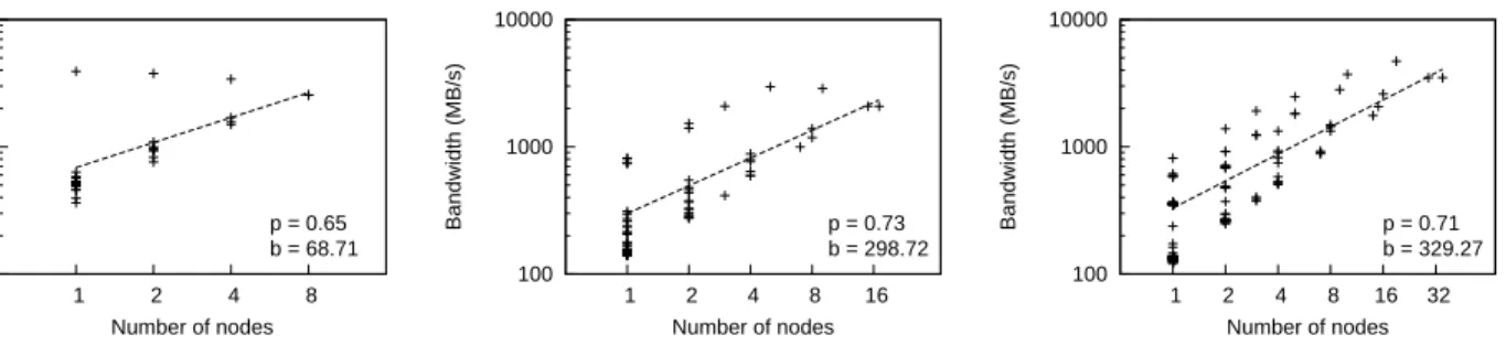
Most software is known to have time-varying behavior [9]. Therefore, we should ask the question whether the Rent ex-ponents measured in Section 3 are constant through time. Figure 2 shows that this is not the case. Here, the traffic trace was divided into intervals of one million cycles each. For each interval a new Rent exponent was estimated. The graphs show, from left to right, the Rent exponent p that was fitted for each of the intervals, the average node band-widthbr (relative to the global average bandwidth b), and a distribution ofpversusbr for all intervals.
The leftmost set of graphs show that the Rent exponent
pis not constant through time: periods of global cation are followed by periods of more localized communi-cation. One should keep in mind though that, if only little traffic is being exchanged on the network, small variations in traffic can cause a large change in the estimated value of p. Therefore, the bandwidthbr, which is plotted in the next set of graphs, is of equal importance. Here we see that momentary bandwidths can be up to ten times the average bandwidth, followed by periods of very little communica-tion. The situation is even more pronounced when we look at individual nodes. This observation supports the claim that a packetized communication network is able to achieve much higher utilization factors than would be the case when using global wiring as dedicated connections. Finally, in the third column we look at the correlation betweenpandb.
Forfft4M, we see large variations inpthroughout the exe-cution. The bandwidth is usually relatively low, with several peaks near the end. This can be explained by the ‘butter-fly’ pattern of the Fast Fourier Transform algorithm, and the way data is distributed across network nodes. At first, each processor works only on data located on its own node. Later, the butterfly pattern expands to include data stored on other nodes, so communication is required. Since there is only limited communication in the first part, the estimated
pvalues are more influenced by ‘noise’: memory accesses not related to the main data, but for instance to synchroniza-tion primitives or operating system structures. The right-most graph shows this: at low communication bandwidths, there are both intervals with highly localized and with global communication. The data streams during high bandwidth phases are much more localized.
For the water.sp benchmark, different behavior can be observed. Periods of high and low communication follow each other in a regular sequence. When bandwidth require-ments are high,premains at around 0.7–0.8. During times that communication rates are lower, the background noise of operating system structure accesses is much more visible and causespto fluctuate. Again, this behavior can be explained by analyzing the algorithm behind thewater.spbenchmark. The program simulates molecular interactions in liquid wa-ter during a number of time steps. Each of the proces-sors is responsible for part of the 512 molecules. Per time step, several phases can be distinguished. The first phase simulates interactions between all molecules and computes the forces they exert on each other. Here communication is global because each molecule influences all other molecules. In the second phase, interactions inside the molecule are computed. This requires no communication since proces-sors should have the data for their ‘own’ molecules cached. Finally, the forces are integrated and molecule velocities and positions are updated, again requiring little communication.
0 0.2 0.4 0.6 0.8 1 0 50 100 150 200 250 Rent exponent
Simulation time (M cycles) barnes, 16 nodes 0 1 2 3 4 5 6 7 8 0 50 100 150 200 250
Per node bandwidth
Simulation time (M cycles) barnes, 16 nodes 0 0.2 0.4 0.6 0.8 1 0 1 2 3 4 5 6 7 8 Rent exponent Bandwidth barnes, 16 nodes 0 0.2 0.4 0.6 0.8 1 0 200 400 600 800 1000 Rent exponent
Simulation time (M cycles) fft4M, 16 nodes 0 1 2 3 4 5 6 0 200 400 600 800 1000
Per node bandwidth
Simulation time (M cycles) fft4M, 16 nodes 0 0.2 0.4 0.6 0.8 1 0 1 2 3 4 5 6 Rent exponent Bandwidth fft4M, 16 nodes 0 0.2 0.4 0.6 0.8 1 0 20 40 60 80 100 120 140 160 Rent exponent
Simulation time (M cycles) radix, 32 nodes 0 0.5 1 1.5 2 2.5 0 20 40 60 80 100 120 140 160
Per node bandwidth
Simulation time (M cycles) radix, 32 nodes 0 0.2 0.4 0.6 0.8 1 0 0.5 1 1.5 2 2.5 Rent exponent Bandwidth radix, 32 nodes 0 0.2 0.4 0.6 0.8 1 0 100 200 300 400 500 600 700 800 Rent exponent
Simulation time (M cycles) ocean.cont, 32 nodes 0 0.2 0.4 0.6 0.8 1 1.2 1.4 0 100 200 300 400 500 600 700 800
Per node bandwidth
Simulation time (M cycles) ocean.cont, 32 nodes 0 0.2 0.4 0.6 0.8 1 0 0.2 0.4 0.6 0.8 1 1.2 1.4 Rent exponent Bandwidth ocean.cont, 32 nodes 0 0.2 0.4 0.6 0.8 1 0 20 40 60 80 100 Rent exponent
Simulation time (M cycles) water.sp, 64 nodes 0 0.2 0.4 0.6 0.8 1 1.2 1.4 1.6 1.8 0 20 40 60 80 100
Per node bandwidth
Simulation time (M cycles) water.sp, 64 nodes 0 0.2 0.4 0.6 0.8 1 0 0.2 0.4 0.6 0.8 1 1.2 1.4 1.6 1.8 Rent exponent Bandwidth water.sp, 64 nodes
Figure 2: Left to right: estimated Rent exponentpand relative per node bandwidth br through time, andp
versus br for all intervals. Top to bottom: barnes and fft4M on 16 nodes, radix and ocean.cont on 32 nodes andwater.sp on 64 nodes
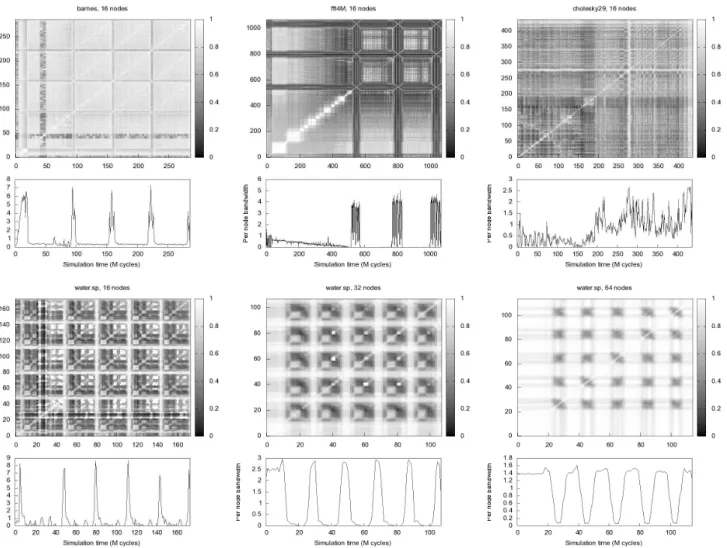
Figure 3: Similarity matrices of all interval pairs per benchmark. The coloring runs from white (simx,y = 1,
equal partitioning), to black (simx,y = 0, dissimilar partitioning). barnes, cholesky29and fft4M are shown for
a 16 node network, andwater.sp for 16, 32 and 64 nodes. Below each, the relative per node bandwidth br is repeated from Figure 2 for reference
5. NODE PLACEMENT
5.1 Optimal placement variation
Just as in VLSI design, the top-down partitioning of the nodes can be a basis for solving the placement problem, in this case by assigning program threads to network nodes, minizing long-distance communication. On the other hand, we just concluded from Figure 2 that network traffic can change drastically through time. We should therefore ask the question: will the optimal node placement change just as drastically? And, when a placement is used that is non-optimal during some of the time, how will this affect perfor-mance?
We try to answer this question using the similarity metric simA,Bdefined in Section 2.3. It provides a way to compare
two partitionings, accounting for bandwidth requirements (i.e., moving low-bandwidth nodes across partitions has lit-tle influence). Figure 3 is constructed by dividing the traffic trace into one million cycle intervals. We again partition the nodes in each of the intervals. The similarity metric simA,B
was then used to compare each pair of intervals. Interval numbers run on both X and Y axes, the square at each in-tersection point is colored according to the value of simx,y:
white when simx,y is one, black for zero. Since the
similar-ity of an interval with itself is always one, all points on the
x=ydiagonal are white.
Again, different applications have clearly different behav-ior. Inbarnes, an N-body simulation program, four similar phases are caused by the simulation to run over four time steps. In each step, a similar calculation is done, involv-ing the same data. The lightly colored squares along the diagonal mean that the partitioning, and thus the commu-nication pattern, remains very similar during intervals of about 60 million cycles (60 intervals of one million cycles each, on either the X or Y axis). Next, a period with a very different and quickly changing communication pattern is en-countered, involving much higher bandwidths. The large, lightly colored squares off the diagonal are also interesting: this means that, for instance, the node placement that is optimal during the 100M-160M cycles interval is very close
to the optimum for the traffic present during the interval from 230M to 280M cycles. For barnes, one node place-ment is therefore very close to optimal for a large fraction of time. This only concerns the low-bandwidth phases of the application though. The high-bandwidth phases, which have much more effect on total performance, have highly erratic communication. Even though the momentary Rent exponent for these high-bandwidth phases is quite low (this is visible in Figure 2), the communication partners change rapidly. Doing a good static node placement forbarnes is therefore not possible.
For thefft4Mbenchmark, we might have concluded from Figure 2 that it has an ‘easy’ communication pattern: only a few high-bandwidth phases which all have a very low Rent exponent, i.e., with highly localized communication. Yet, in Figure 3, we see that these same phases are very unlike their immediately neighboring phases. So although commu-nication is highly localized when viewed at short intervals, a little while later the communication partners have changed causing the communication at a longer time scale to be much more global.
The lower half of Figure 3 shows the similarity graphs for thewater.spbenchmark when scaling the network size. On a 64-node network, comparison of the similarity matrix with the bandwidth requirements shows that for this benchmark, the high-bandwidth periods correspond to large white re-gions in the similarity graph. So for water.sp, a single good placement does exist that is effective throughout all high-bandwidth phases of the application. This is true on all networks, although the fraction of time spent in peri-ods of intense communication increases significantly when moving to larger networks. We can assume that during the low-bandwidth periods (communication now only consists of some ‘random’ accesses to operating system structures, therefore these periods correspond to darkly colored regions) the processors are mainly performing computation on local data. Since on larger networks, there are more processors to do the same work, the computation time decreases (the black periods shorten, from 30M cycles on 16 processors to 10M cycles on 64 processors). The total program run-time, on the other hand, remains at just above 100M cycles. This shows that thewater.spapplication does not scale fa-vorably to 64 processors, i.e., although more resources are available, the time required to compute the solution does not reduce accordingly, taking into account that the input data remains constant at 512 molecules. Communication is the limiting factor here, but we also see that communica-tion is very regular and it should therefore be possible to solve this bottleneck by designing a suitable interconnection topology.
5.2 Optimality of a single placement
To asses the optimality of a given placement, derived from a single partitioning, we use the suitability metric defined in Section 2. suitP,A determines the suitability of the
par-titioningP for the traffic pattern in intervalA, while suitP
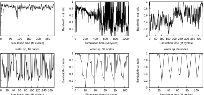
provides a global metric. Figure 4 plots suitP,A for the
op-timalpartitioning, this is the partitioning with the maximal
suitP. It can be shown that this partitioning is equal to the
one made on the global traffic matrix, which was done in Section 3.
As could be expected from Figure 3, the optimal partition-ing forbarnesis very close to optimal for most of the time.
Benchmark suitA for optimal partitioning
16 nodes 32 nodes 64 nodes
barnes 0.84 0.89 0.90 cholesky 0.69 0.85 0.93 cholesky29 0.63 0.81 0.93 fft 0.78 0.89 0.94 fft4M 0.38 0.79 0.91 fftscale 0.78 0.91 lu 0.86 0.91 0.95 luscale 0.86 0.87 0.88 ocean.cont 0.95 0.97 0.98 ocean.contscale 0.95 0.90 0.90 radix 0.84 0.90 0.93 radixscale 0.87 0.90 0.88 water.nsq 0.82 0.92 0.92 water.sp 0.77 0.92 0.94
Table 3: Suitability of the optimal partitioning, av-eraged over time, for all benchmarks and network sizes
Some drops are visible, not surprisingly, during the periods of high, irregular communication. fft4Mandcholeskyhave irregular communication all of the time, no single placement can therefore be optimal. The optimal partitioning chosen for water.sp, corresponds to that of the periods of high communication. This is the case even in the 16-node case, even though there the high-bandwidth phases are very short. Still, since most of the data is exchanged during those peri-ods, they will influence performance most.
Table 3 summarizes the global suitability suitP for the
best partitioning, for all benchmarks and all network sizes.
fft4Mon 16 nodes has very irregular communication causing its suitP to be only 0.38. Forwater.sp, the relative
frac-tion of regular communicafrac-tion increases when making the network larger, suitP follows this trend by going from 0.77
to 0.94. ocean.conthas extremely regular communication which is causing it to score 0.95–0.98 on all network sizes.
6. FUTURE WORK
This analysis presents the network designer with a new tool for analyzing network traffic and communication re-quirements. Since Rent’s rule essentially remains valid when using packetized on-chip networks, many of the ideas based on Rent’s rule, such as placement, a priori estimation of ‘wirelength’ (now routing distance) and congestion (of pack-ets instead of wires), can be re-used. Also, by highlighting the temporal variability of network traffic, it becomes clear that, when the scope and complexity of single chips expands to include more, and more diverse, applications, reconfigu-ration, in one of its forms, will probably gain importance and should therefore be the object of further exploration.
7. CONCLUSIONS
We have shown that, when ad-hoc global wiring struc-tures are being replaced by packetized communication over regular on-chip networks, Rent’s rule remains applicable: a power-law relationship is clearly visible when partitioning network nodes and comparing their size versus their external bandwidth. The exponent does change when the network size is increased. For small networks this can be attributed
0 0.2 0.4 0.6 0.8 1 0 50 100 150 200 250
Bandwidth cut ratio
Simulation time (M cycles) barnes, 16 nodes 0 0.2 0.4 0.6 0.8 1 0 200 400 600 800 1000
Bandwidth cut ratio
Simulation time (M cycles) fft4M, 16 nodes 0 0.2 0.4 0.6 0.8 1 0 50 100 150 200 250 300 350 400
Bandwidth cut ratio
Simulation time (M cycles) cholesky29, 16 nodes 0 0.2 0.4 0.6 0.8 1 0 20 40 60 80 100 120 140 160
Bandwidth cut ratio
Simulation time (M cycles) water.sp, 16 nodes 0 0.2 0.4 0.6 0.8 1 0 20 40 60 80 100
Bandwidth cut ratio
Simulation time (M cycles) water.sp, 32 nodes 0 0.2 0.4 0.6 0.8 1 0 20 40 60 80 100
Bandwidth cut ratio
Simulation time (M cycles) water.sp, 64 nodes
Figure 4: Suitability of the optimal partitioning through time forbarnes, cholesky29and fft4M on a 16 node network, and forwater.sp on 16, 32 and 64 node networks
to the limited number of data points, which precludes a reli-able estimate of the Rent exponent. For larger networks, the higher than expected exponent shows that the distribution of work and data across network nodes was not always done optimally in the SPLASH-2 benchmarks we studied. Still, from the Rent exponent, and the partitioning with which it was derived, a lot can be learned about the communication behavior of an application. Most of this behavior can be traced back to the algorithm executed by the program, and the way data is located across network nodes. Repeating this analysis on different time scales also learns that network traffic can often change dramatically through time, and that static node placements, for several important applications, may no longer be sufficient.
8. ACKNOWLEDGMENTS
This paper presents research results of the Inter-university Attraction Poles program photonics@be (IAP–Phase VI), initiated by the Belgian State, Prime Minister’s Service, Sci-ence Policy Office.
9. REFERENCES
[1] P. Christie and D. Stroobandt. The interpretation and application of Rent’s rule.IEEE Transactions on Very
Large Scale Integration Systems, 8(6):639–648,
Dec. 2000.
[2] W. J. Dally and B. Towles. Route packets, not wires: On-chip interconnection networks. InDesign
Automation Conference, pages 684–689, June 2001.
[3] R. P. Dick, D. L. Rhodes, and W. Wolf. TGFF: task graphs for free. InProceedings of the 6th International
Workshop on Hardware/Software Codesign,
pages 97–101, Seattle, Washington, Mar. 1998. [4] D. Greenfield, A. Banerjee, J.-G. Lee, and S. Moore.
Implications of Rent’s rule for NoC design and its
fault-tolerance. InProceedings of the First
International Symposium on Networks-on-Chips,
pages 283–294, Princeton, New Jersey, May 2007. [5] W. Heirman, J. Dambre, I. Artundo, C. Debaes,
H. Thienpont, D. Stroobandt, and
J. Van Campenhout. Predicting the performance of reconfigurable optical interconnects in distributed shared-memory systems.Photonic Network
Communications, 15(1):25–40, Feb. 2008.
[6] B. S. Landman and R. L. Russo. On a pin versus block relationship for partitions of logic graphs.IEEE
Transactions on Computers, C-20(12):1469–1479,
Dec. 1971.
[7] P. S. Magnusson, M. Christensson, J. Eskilson, D. Forsgren, G. Hallberg, J. Hogberg, F. Larsson, A. Moestedt, and B. Werner. Simics: A full system simulation platform.IEEE Computer, 35(2):50–58, Feb. 2002.
[8] N. Selvakkumaran and G. Karypis. Multi-objective hypergraph partitioning algorithms for cut and maximum subdomain degree minimization.IEEE Transactions on Computer-Aided Design of Integrated
Circuits and Systems, 25(3):504– 517, Mar. 2006.
[9] T. Sherwood, E. Perelman, G. Hamerly, and B. Calder. Automatically characterizing large scale program behavior. InProceedings of the 10th
International Conference on Architectural Support for
Programming Languages and Operating Systems,
pages 45–57, San Jose, California, Oct. 2002. [10] S. C. Woo, M. Ohara, E. Torrie, J. P. Singh, and
A. Gupta. The SPLASH-2 programs: Characterization and methodological considerations. InProceedings of the 22th International Symposium on Computer
Architecture, pages 24–36, Santa Margherita Ligure,