Digital Commons@Georgia Southern
Biostatistics Faculty Publications
Biostatistics, Department of
9-30-2016
Estimation of
P(X > Y)
When
X
and
Y
Are
Dependent Random Variables Using Different
Bivariate Sampling Schemes
Hani M. Samawi
Georgia Southern University, [email protected]
Amal Helu
Carnegie Mellon University
Haresh Rochani
Georgia Southern University, [email protected]
Jingjing Yin
Georgia Southern University, [email protected]
Daniel Linder
Georgia Southern University, [email protected]
Follow this and additional works at:
https://digitalcommons.georgiasouthern.edu/biostat-facpubs
Part of the
Biostatistics Commons
, and the
Public Health Commons
This article is brought to you for free and open access by the Biostatistics, Department of at Digital Commons@Georgia Southern. It has been accepted for inclusion in Biostatistics Faculty Publications by an authorized administrator of Digital Commons@Georgia Southern. For more information, please [email protected].
Recommended Citation
Samawi, Hani M., Amal Helu, Haresh Rochani, Jingjing Yin, Daniel Linder. 2016. "Estimation ofP(X > Y)WhenXandYAre Dependent Random Variables Using Different Bivariate Sampling Schemes."Communications for Statistical Applications and Methods, 23 (5): 385-397: Korean Statistical Society and Korean International Statistical Society. doi: 10.5351/CSAM.2016.23.5.385 https://digitalcommons.georgiasouthern.edu/biostat-facpubs/147
Estimation of
P
P
P
(X
(X
(X
>
>
>
Y
Y)
Y)
)
when
X
X
X
and
Y
Y
Y
are dependent
random variables using different bivariate sampling
schemes
Hani M. Samawi1,a, Amal Helub, Haresh D. Rochania, Jingjing Yina, Daniel Lindera
aDepartment of Biostatistics, Jiann-Ping Hsu College of Public Health, Georgia Southern University, USA;bCarnegie Mellon University, Qatar
Abstract
The stress-strength models have been intensively investigated in the literature in regards of estimating the reliabilityθ=P(X>Y) using parametric and nonparametric approaches under different sampling schemes when
XandYare independent random variables. In this paper, we consider the problem of estimatingθwhen (X,Y) are dependent random variables with a bivariate underlying distribution. The empirical and kernel estimates of θ=P(X>Y), based on bivariate ranked set sampling (BVRSS) are considered, when (X,Y) are paired dependent continuous random variables. The estimators obtained are compared to their counterpart, bivariate simple random sampling (BVSRS), via the bias and mean square error (MSE). We demonstrate that the suggested estimators based on BVRSS are more efficient than those based on BVSRS. A simulation study is conducted to gain insight into the performance of the proposed estimators. A real data example is provided to illustrate the process.
Keywords: bivariate simple random sampling, bivariate ranked set sampling, empirical and kernel estimation, reliability, bias, mean square error
1. Introduction
In the literature, inference aboutθ=P(X>Y) has been extensively studied. In the area of reliability
for a system with strength X and stressY, inference aboutθ = P(X>Y) as a measure of
compo-nent reliability is crucial (Kotzet al., 2003). In medicine, the parameterθcan be interpreted as the
effectiveness of treatmentYifXandYare the outcomes of a control and an experimental treatment,
respectively (Ventura and Racugno, 2011). This quantity is also related to the Receiver Operating
Characteristic (ROC) curves, whereθis interpreted as an index of accuracy (Zhou, 2008). Therefore,
the estimation ofθ=P(X>Y) has a wide range of applications in the literature.
This problem has been investigated from different points of views. For parametric inference,
assuming X andY have independent exponential distributions, see Enis and Geisser (1971), Awad
et al. (1981), Tong (1974), and Johnson (1975). Moreover, Liet al. (1999) studied the problem of
estimatingθ = P(X>c) based on simple random sampling (SRS) and ranked set sampling (RSS).
They showed that the estimators ofθ=P(X>c) based on RSS were more efficient than those based
on SRS in terms of the variances.
In many situations the parameterθmay not be available in a closed form. This makes it difficult (if
at all feasible) to find a reparameterization involvingθto use any classical approaches. In particular,
1Corresponding author: Department of Biostatistics, Karl E. Peace Center for Biostatistics, Jiann-Ping Hsu College of Public Health, Georgia Southern University, 8015, Statesboro, GA 30460, USA. E-mail: [email protected]
Published 30 September 2016/ journal homepage: http://csam.or.kr c
the use of the profile likelihood may be difficult if this reparameterization is not available
(D´ıaz-Franc´es and Montoya, 2013). Alternative inferential approaches that overcome this difficulty are
Bayesian inference, nonparametric estimation and the use of bootstrap methods, which can be used
for obtaining confidence and credible intervals for the parameter of interest (AL-Hussainiet al., 1997;
Baklizi and Abu-Dayyeh, 2003; Baklizi and Eidous, 2006; Rubio and Steel, 2013; Zhou, 2008).
Currently, many authors have tried to estimateθin the case whereXandYare dependent random
variables. For example Barbiero (2012) assumed that (X,Y) are jointly normally distributed; Rubio
and Steel (2013) assumed thatXandYare marginally distributed as a skewed scale mixture of normal
and constructed the corresponding joint distribution using a Gaussian copula; Domma and Giordano
(2013) constructed the joint distribution of (X,Y) using a Farlie-Gumbel-Morgenstern copula with
marginal distributions belonging to the Burr system; Domma and Giordano (2012) considered Dagum distributed marginals and constructed their joint distribution using a Frank copula; among others
(Guptaet al., 2013; Nadarajah, 2005). In these papers, the importance of taking the assumption of
dependence betweenXandYinto consideration is illustrated using simulated and real data sets.
In most cases SRS is considered for estimatingθ, however, some variations of RSS and SRS
with concomitant variable were considered for estimatingθ, see for example Sengupta and Mukhuti
(2008) and Muttlaket al. (2010). RSS has been applied in many fields, including but not limited to
agricultural, environmental studies and recently in human populations. The motivation for using RSS is that in some cases quantification (the actual measurement) of a sampling unit can be more costly than the physical acquisition of the unit. For example, as stated by Samawi and Al-Sagheer (2001), the level of bilirubin in the blood of infants can be ranked visually by observing: i) color of the face, ii) color of the chest, iii) color of lower part of the body, iv) color of terminal parts of the whole body. As the level of bilirubin in the blood increases, the yellowish discoloration goes from i) to iv) (Samawi and Al-Sagheer, 2001). Also, in some circumstances, considerable cost savings can be achieved if the number of measured sampling units are only a small fraction of the number of available units, but all units contribute to the information content of the measured units, which is the case for RSS. RSS was first introduced by McIntyre (1952). RSS has been shown to be superior to the standard SRS for estimating some population parameters. More details about RSS and its variations are available in Kauret al. (1995), Patilet al. (1999), Samawiet al. (1996) and Samawi and Muttlak (1996, 2001). However, all variations of RSS sampling methods, preformed their ranking on one and only one of the study variables.
For multiple characteristics estimation, few authors worked in this area such as Patilet al.(1993,
1994) and Norriset al.(1995). They used a bivariate ranked set sampling procedure by ranking only
on one of the characteristics (XorY). However, bivariate ranked set sampling (BVRSS) by ranking
on both characteristics (XandY) was introduced by Al-Saleh and Zheng (2002). They indicated that
BVRSS procedure could easily be extended to a multivariate one. The focus of this paper is to show that the use of BVRSS will substantially improve the performance of the empirical and the kernel
estimators forθanalytically and by simulation. Section 2 discusses the empirical estimator ofθand
its properties, while Section 3 discusses the kernel estimator and its properties. Section 4 provides the simulation study. In Section 5 we illustrated the procedure using a real data set. Section 6 provides the final remarks.
2. Empirical estimation of
θ
θ
θ
=
=
=
P
P
P
(
(
(
X
X
X
>
>
>
Y
Y
Y
)
)
)
2.1. Empirical estimation using BVSRS
variable with joint probability density function (p.d.f.) fX,Y(x,y). Thus θ= ∫ ∞ −∞ ∫ x −∞ fX,Y(x,y)dydx. (2.1)
An alternative approach is to setW =X−Yand then we have
θ=P(W >0)= ∫ ∞
0
fW(w)dw=1−FW(0)=SW(0), (2.2)
where fW(w),FW(0) andSW(0) are the density, cumulative distribution function (c.d.f.), and the
sur-vival function ofW, respectively. Let{(X1,Y1),(X2,Y2), . . . ,(Xn,Yn)}be an independent BVSRS from
fX,Y(x,y). The empirical estimator ofθbased on these BVSRS for equation (2.1) is:
ˆ
θBVS RS = ∑n
i=1I(Yi<Xi)
n (2.3)
and for equation (2.2) is
ˆ
θBVS RS(W) = ∑n
i=1I(Wi>0)
n . (2.4)
Note that both estimators are unbiased and with variancesθ(1−θ)/nandSW(0)(1−SW(0))/n,
respec-tively. Moreover, ˆθBVS RS and ˆθBVS RS(W)are strongly consistent estimators ofθ, or ˆθBVS RS
a.s.
−−→θand ˆ
θBVS RS(W) a.s.
−−→θ, and are also asymptotically normally distributed, implying that √n(ˆθBVS RS −θ)
d − → N(0, θ(1−θ)) and √n(ˆθBVS RS(W)−θ) d − → N(0,SW(0)(1−SW(0))), as n→ ∞, as shown by Montoya and Rubio (2014).
2.2. Empirical estimation using BVRSS
Based on Al-Saleh and Zheng (2002) description, a BVRSS can be obtained as follows: suppose
(X,Y) is a bivariate random vector with the joint p.d.f. f(x,y).
Step 1. A random sample of sizer4is identified from the population and randomly allocated intor4
pools of sizer4each so that each pool is a square matrix withrrows andrcolumns.
Step 2. In the first pool, rank each set (row) by a suitable method of ranking with respect to (w.r.t.)
the first characteristic (X). Then from each row identify the unit with the smallest rankw.r.t.
X.
Step 3. Rank therminima obtained in Step 2, in a similar manner butw.r.t.the second characteristic
(Y). Then identify and measure the unit with the smallest rankw.r.t.Y. This pair of
mea-surements (x,y), which is resembled by the label (1, 1), is the first element of the BVRSS
sample.
Step 4. Repeat Steps 2 and 3 for the second pool, but in Step 3, the pair that corresponds to the
second smallest rankw.r.t.the second characteristic (Y) is chosen for actual measurement
(quantification). This pair is resembled by the label (1, 2).
The above procedure produces a quantified BVRSS of sizer2. The procedure can be repeated
mtimes to obtain a sample of sizen = mr2. In sampling notation, assume that a random sample
of sizemr4is identified (no measurements were taken) from a bivariate probability density function,
say fX,Y(x,y) : (x,y)∈R2, with meansµxandµy, variancesσ2xandσ2yand correlation coefficientρ. Following the Al-Saleh and Zheng (2002) definition of BVRSS, then [(X[i](j)k,Y(i)[j]k),i=1,2, . . . ,r;
j=1,2, . . . ,r; andk=1,2, . . . ,m] denotes the BVRSS. Now, let fX[i](j),Y(i)[j](x,y) be the joint p.d.f. of [(X[i](j)k,Y(i)[j]k), k=1,2, . . . ,m]. Al-Saleh and Zheng (2002), withm=1, showed that
1 r2 r ∑ j=1 r ∑ i=1 f[i](j),(i)[j](x,y)= fX,Y(x,y). (2.5)
Then using these BVRSSs, for equation (2.1), we propose the following empirical estimators ofθ:
ˆ θBVRS S = ∑m k=1 ∑r i=1 ∑r j=1I ( X[i](j)k>Y(i)[j]k ) n ; n=mr 2 (2.6)
and for equation (2.2)
ˆ θBVRS S(W)= ∑m k=1 ∑r i=1 ∑r j=1I(Wi,j,k>0) n , (2.7) whereWi,j,k=X[i](j)k−Y(i)[j]k.
Using equation (2.5) we have the following results.
Theorem 1.
(a) θˆBVRS S andθˆBVRS S(W)are unbiased estimators ofθ.
(b) Var(θˆBVRS S ) =1 n θ(1−θ)− ∑r i=1 ∑r j=1(θi j−θ)2 r2 and Var(θˆBVRS S(W) ) =1 n SW(0)(1−SW(0))− ∑r i=1 ∑r j=1 ( SW(i,j)(0)−SW(0) )2 r2 , whereθi j=P(X[i](j) >Y(i)[j]), and SW(i,j)(0)=P(X[i](j)−Y(i)[j]>0), i=1,2, . . . ,r, j=1,2, . . . ,r. Proof: The proof of Theorem 1 is straightforward and it is omitted from the paper.
Note that it is clear that the empirical estimate based on BVRSS has smaller variance than using
BVSRS for estimatingθ.
Theorem 2. For fixed r and as m→ ∞, and hence n→ ∞, we have (a) θˆBVRS S and θˆBVRS S(W)are strongly consist estimators ofθ, orθˆBVRS S
a.s. −−→θand θˆBVRS S(W) a.s. −−→ θ. (b) √n(ˆθBVRS S −θ) d − → N(0,G) and √n(ˆθBVRS S(W)−θ) d − → N(0,GS), where G = θ(1−θ) − {∑r i=1 ∑r j=1(θi j−θ)2}/r2and G=SW(0)(1−SW(0))− {∑ri=1 ∑r j=1(SW(i,j)(0)−SW(0))2}/r2. Proof: The proof follows by the law of large number and the central limit theorem.
3. Kernel estimation of
θ
θ
θ
=
=
=
P
P
P
(
(
(
X
X
X
>
>
>
Y
Y
Y
)
)
)
3.1. Kernel estimation using BVSRS
Montoya and Rubio (2014) proposed nonparametric kernel estimators forθfrom equations (2.1) and
(2.2) as follows: LetHbe a symmetric, positive definite, 2×2 bandwidth matrix andk2 be a
two-dimensional kernel function (Parzen, 1962). DefinekH(t) = (detH)−1/2k2
(
H1/2t),t∈R2, where,
t={t1 =x−X,t2=y−Y}. Using kernel density estimation, then we will have the kernel estimations
forθin equations (2.1) and (2.2) are defined as
ˆ θK(BVS RS)= ∫ ∞ −∞ ∫ x −∞ 1 n n ∑ i=1 kH(x−Xi,y−Yi)dydx = ∫ ∞ −∞ ∫ t1 −∞ 1 nfˆBVS RS(t1,t2)dt1dt2 (3.1) and ˆ θK(BVS RS(W))= 1 nh n ∑ i=1 ∫ ∞ 0 k1 (w−W i h ) dw =1−1 n n ∑ i=1 K1 (W i h ) = ∫ ∞ 0 ˆ fBVS RS(W)(w)dw =1−FˆBVS RS(0), (3.2) where,K1(w/h)=(1/h) ∫∞
0 k1(w/h)dw,k1is one-dimensional kernel function with a bandwidthh>0.
One of the most common choices of kernel functions for one or two-dimensional kernels are the
univariate and the bivariate normal densities, respectively. For the choice of the bandwidth matrixh
andHwe refer to Montoya and Rubio (2014) for full discussion. Moreover, they showed that, under
some regularity conditions, ˆθK(BVS RS)
P
−→ θ(weakly consistent estimator) and ˆθK(BVS RS(W))
a.s.
−→ θ
(strong consistent estimator).
3.2. Kernel estimation using BVRSS
Again, let [(X[i](j)k,Y(i)[j]k), i = 1,2, . . . ,r; j = 1,2, . . . ,r; and k = 1,2, . . . ,m] be a BVRSS from (X,Y) with f(x,y). Similarly, define kH(t) = (detH)−1/2k2(H1/2t),t∈R2.Then using the BVRSS
samples, we propose the following kernel estimators ofθ:
ˆ θK(BVRS S)= ∑m k=1 ∑r i=1 ∑r j=1 ∫∞ −∞ ∫x −∞kH ( x−X[i](j)k,y−Y(i)[j]k ) dydx n = ∫ ∞ −∞ ∫ x −∞ ˆ fBVRS S(t1,t2)dt1dt2; n=mr2, (3.3)
for equation (2.1) and ˆ θK(BVRS S(W))= ∑m k=1 ∑r i=1 ∑r j=1 ∫∞ 0 K1 (w−Wi j h ) dw nh =1−1 n m ∑ k=1 r ∑ i=1 r ∑ j=1 K1 ( w−Wi j h ) = ∫ ∞ 0 ˆ fBVRS S(W)(w)dw =1−FˆBVRS S(0) (3.4)
for equation (2.2), whereWi jk =X[i](j)k−Y(i)[j]k.
Theorem 3. (a) E(θˆK(BVRS S) ) =E(θˆK(BVS RS) ) ,E(θˆK(BVRS S(W)) ) =E(θˆK(BVS RS(W)) ) , (b) Var(θˆK(BVRS S) ) = Var(θˆK(BVS RS) ) − 1 nr2 r ∑ i=1 r ∑ j=1 ( Ei j−E )2 =V1, (c) Var(θˆK(BVRS S(W)) ) = Var(θˆK(BVS RS(W)) ) − 1 nr2 r ∑ i=1 r ∑ j=1 ( Di j−D )2 =V2, where, Ei j =EX[i](j),Y(i)[j] [∫ ∞ −∞ ∫ u −∞KH ( u−X[i](j), ν−Y(i)[j] ) dνdu ] , E=EX,Y [∫ ∞ −∞ ∫ u −∞KH (u−X, ν−Y)dνdu ] , Di j =EWi j [∫ ∞ 0 1 hk1 ( w−Wi j h ) dw ] , and D=EW [∫ ∞ 0 1 hk1 (w−W h ) dw ] . Proof: (a) E(θˆK(BVRS S) ) =E ∑m k=1 ∑r i=1 ∑r j=1 ∫∞ −∞ ∫u −∞KH ( u−X[i](j)k, ν−Y(i)[j]k ) dνdu n =E ∑r i=1 ∑r j=1 ∫∞ −∞ ∫u −∞KH ( u−X[i](j)k, ν−Y(i)[j]k ) dνdu r2 = 1 r2 ∫ ∞ −∞ ∫ ∞ −∞ r ∑ i=1 r ∑ j=1 ∫ ∞ −∞ ∫ u −∞KH ( u−X[i](j)k, ν−Y(i)[j]k ) dνdu f[i](j),(i)[j](x,y)dxdy = ∫ ∞ −∞ ∫ ∞ −∞ [∫ ∞ −∞ ∫ u −∞ KH(u−x, ν−y)dudν ] 1 r2 r ∑ i=1 r ∑ j=1 f[i](j),(i)[j](x,y)dxdy,
then by using (2.5), we have
E(θˆK(BVRS S) ) = ∫ ∞ −∞ ∫ ∞ −∞ (∫ ∞ −∞ ∫ u −∞KH (u−x, ν−y)dudν ) f(x,y)dxdy =E(θˆK(BVS RS) )
Similarly, we can show thatE(ˆθK(BVRS S(W)))=E(ˆθK(BVS RS(W))). (b) Var(θˆK(BVRS S) ) =Var mr12 m ∑ k=1 r ∑ i=1 r ∑ j=1 ∫ ∞ −∞ ∫ u −∞ KH ( u−X[i](j)k, ν−Y(i)[j]k ) dνdu = 1 mr4Var r ∑ i=1 r ∑ j=1 ∫ ∞ −∞ ∫ u −∞ KH ( u−X[i](j)k, ν−Y(i)[j]k ) dνdu = 1 mr4 r ∑ i=1 r ∑ j=1 Var [∫ ∞ −∞ ∫ u −∞KH ( u−X[i](j)k, ν−Y(i)[j]k ) dνdu] = 1 mr4 r ∑ i=1 r ∑ j=1 ∫ ∞ −∞ ∫ ∞ −∞ [∫ ∞ −∞ ∫ u −∞KH ( u−X[i](j)k, ν−Y(i)[j]k ) dudν−Ei j ]2 f[i](j),(i)[j](x,y)dxdy, where, Ei j=EX[i](j),Y(i)[j] (∫ ∞ −∞ ∫ u −∞KH ( u−X[i](j), ν−Y(i)[j] ) dudν ) then, Var(θˆK(BVRS S) ) = 1 mr4 r ∑ i=1 r ∑ j=1 ∫ ∞ −∞ ∫ ∞ −∞ [∫ ∞ −∞ ∫ u −∞KH ( u−X[i](j)k, ν−Y(i)[j]k ) dudν−Ei j±E ]2 f[i](j),(i)[j](x,y)dxdy = 1 mr4 r ∑ i=1 r ∑ j=1 ∫ ∞ −∞ ∫ ∞ −∞ [∫ ∞ −∞ ∫ u −∞KH ( u−X[i](j)k, ν−Y(i)[j]k ) dudν−E ]2 f[i](j),(i)[j](x,y)dxdy −2(Ei j−E ) ∫ ∞ −∞ ∫ ∞ −∞ [∫ ∞ −∞ ∫ u −∞KH ( u−X[i](j)k, ν−Y(i)[j]k ) dudν−E ] f[i](j),(i)[j](x,y)dxdy +(Ei j−E )2} = 1 mr4 ∫ ∞ −∞ ∫ ∞ −∞ [∫ ∞ −∞ ∫ u −∞ KH(u−x, ν−y)dudν−E ]2 1 r2 r ∑ i=1 r ∑ j=1 f[i](j),(i)[j] (x,y)dxdy − 1 mr4 r ∑ i=1 r ∑ j=1 ( Ei j−E )2 , where,E=EX,Y( ∫∞ −∞ ∫u −∞KH(u−X, ν−Y)dudν). Using (2.5) again, we have
Var(θˆK(BVRS S) ) = Var(θˆK(BVS RS) ) − ( 1 mr4 )∑r i=1 r ∑ j=1 ( Ei j−E )2 .
(c) Can be proved similarly.
As in Montoya and Rubio (2014), and under the same assumptions, we need to show that ˆθK(BVS RS)
and ˆθK(BVS RS(w))consistent estimators forθ.
Theorem 4. Assume that the two-dimensional kernel function k2 is bounded on R2 and the
one-dimensional kernel function k1is bounded onRwith respect to L2and L1the distances
L2(u)=sup
∥t∥≥u
k2(t) and L1(u)=sup
|t|≥u
k1(t),
for u ≥0.Let the bandwidth satisfy h>0, h−→0, n=mr2, nh2 −→ ∞as n−→ ∞,and hence as
m−→ ∞.For the bivariate case, define the bandwidth matrix H=diag(h). Assuming that the same bandwidth is used in both fˆBVRS S(x,y)and fˆBVS RS(x,y)and in both fˆBVRS S(W)(w)and fˆBVS RS(W)(w),
then if one of the following conditions stated by Montoya and Rubio (2014), Silverman (1986) and Wand and Jones (1995), holds
1. |t|k1(t)−→0as|t| −→ ∞;∥t∥2 k2(t)−→0as∥t∥ −→ ∞and fX,Y and fWare almost surely
continuous. 2. fWis bounded; fX,Yis bounded. 3. ∫0∞L1(u)du<∞; ∫∞ 0 uL2(u)du<∞. We haveθˆK(BVRS S) p −→θandθˆK(BVRS S(W)) p −→θ.
Proof: First, we note that MSE(θˆK(BVRS S) ) =E[θˆK(BVRS S)−θ 2] =Bias(θˆK(BVRS S) )2 +Var(θˆK(BVRS S) ) and MSE(θˆK(BVRS S)(W) ) =E[θˆK(BVRS S)(W)−θ 2] =Bias(θˆK(BVRS S)(W) )2 +Var(θˆK(BVRS S)(W) ) .
However, by Theorem 3 we have Bias(θˆK(BVRS S) ) =Bias(θˆK(BVS RS) ) , Bias(θˆK(BVRS S)(W) ) =Bias(θˆK(BVS RS)(W) ) , and Var(θˆK(BVRS S) ) <Var(θˆK(BVS RS) ) , Var(θˆK(BVRS S)(W) ) <Var(θˆK(BVS RS)(W) ) .
Montoya and Rubio (2014) showed that, MSE(θˆK(BVRS S) ) −→0 and MSE(θˆK(BVRS S(W)) ) −→0 and then ˆ θK(BVS RS) p −→θ and θˆK(BVS RS(W)) p −→θ.
However, MSE(θˆK(BVRS S) ) <MSE(θˆK(BVS RS) ) −→0 and MSE(θˆK(BVRS S(W)) ) <MSE(θˆK(BVS RS(W)) ) −→0. Therefore, ˆ θK(BVRS S) p −→θ and θˆK(BVRS S(W)) p −→θ.
Moreover, by the central limit theorem, we have
√ n(θˆK(BVRS S)−θ ) d −→N(0,nV1) and √ n(θˆK(BVRS S(W))−θ ) d −→N(0,nV2). 4. Simulation studies
We conduct a computer simulations to gain insight into the efficiency of estimatingθ. Placketts class of
bivariate distribution with fixed marginal distribution functionsF(x) andG(x) are used to investigate
the performance of the proposed estimators. The Placketts joint c.d.f is given by
H(x,y)= S(x,y)−[S2(x,y)−4ψ(ψ−1)F(x)G(y)] 1 2 2 (ψ−1) , ifψ,1, F(x)G(y), ifψ=1,
whereS(x,y) = 1+(ψ−1)[F(x)+G(y)]and the parameterψgoverns the dependence betweenX
andY. The reason for choosing this class of bivariate distributions is that it covers the full range of
dependency. For example, in case ofU(0,1) marginal distributions, we have the following:
(a) ψ→0⇒X=1−Y, (b) ψ=1⇒XandYare independent, (c) ψ→ ∞ ⇒X=Y.
For more detailed description of Placketts distribution and its random generation, see Johnson (1987).
Four types of dependencies from strongly negative to strongly positive corresponding toψ =
0.1,1.0,2.0,10.0 and two marginal distributions, exponential with mean (µ)=0.5 or 1.0, and gamma
with scale parameterβ=1 or 2 and shape parameterλ=3 are considered. The performance of the
estimators ofθis investigated forr = 2,3,4 andm = 20, therefore the sample sizes used aren =
80,180 and 320. However, we present the results of only set sizesr=3 and 4 to reduce the number
of tables in our simulation, since the other cases provide similar results. Using 5,000 replications,
we estimate the bias and mean square errors (MSE) for the estimators ofθ. The bound on the error
of estimation (using 95% confidence level) is approximately±0.013. The relative efficiency of using
BVRSS relative to using BVSRS for estimatingθis defined by REF=MSE(BVSRS)/MSE (BVRSS).
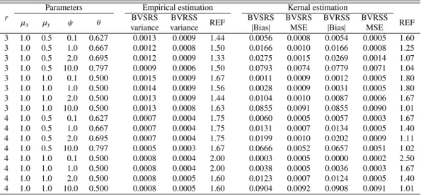
Our simulation indicates that using BVRSS for estimatingθis at least more efficient for all
pre-sented cases in Tables 1 and 2. The relative efficiency is ranging from 1.02 to 2.28 depending on the
strength and the direction of the dependency betweenXandY and the underlying marginal
distribu-tions. However, increasing the set sizerincreases the efficiency. However, increasing the cycle size
Table 1:Performance of empirical and kernel estimators for two exponential marginal distribution andm=20
r
Parameters Empirical estimation Kernal estimation
µx µy ψ θ BVSRS BVRSS REF BVSRS BVSRS BVRSS BVRSS REF
variance variance |Bias| MSE |Bias| MSE 3 1.0 0.5 0.1 0.627 0.0013 0.0009 1.44 0.0056 0.0008 0.0054 0.0005 1.60 3 1.0 0.5 1.0 0.667 0.0012 0.0008 1.50 0.0166 0.0010 0.0166 0.0008 1.25 3 1.0 0.5 2.0 0.695 0.0012 0.0009 1.33 0.0275 0.0015 0.0269 0.0014 1.07 3 1.0 0.5 10.0 0.797 0.0009 0.0006 1.50 0.0793 0.0074 0.0779 0.0071 1.04 3 1.0 1.0 0.1 0.500 0.0015 0.0009 1.67 0.0011 0.0009 0.0012 0.0005 1.80 3 1.0 1.0 1.0 0.500 0.0014 0.0009 1.56 0.0028 0.0009 0.0031 0.0005 1.80 3 1.0 1.0 2.0 0.500 0.0013 0.0009 1.44 0.0104 0.0010 0.0087 0.0006 1.67 3 1.0 1.0 10.0 0.500 0.0013 0.0008 1.63 0.0855 0.0091 0.0855 0.0090 1.01 4 1.0 0.5 0.1 0.627 0.0007 0.0004 1.75 0.0060 0.0005 0.0057 0.0003 1.67 4 1.0 0.5 1.0 0.667 0.0007 0.0004 1.75 0.0131 0.0007 0.0134 0.0005 1.40 4 1.0 0.5 2.0 0.695 0.0007 0.0004 1.75 0.0199 0.0010 0.0202 0.0009 1.11 4 1.0 0.5 10.0 0.797 0.0005 0.0003 1.67 0.0666 0.0052 0.0657 0.0051 1.02 4 1.0 1.0 0.1 0.500 0.0008 0.0004 2.00 0.0003 0.0005 0.0000 0.0002 2.50 4 1.0 1.0 1.0 0.500 0.0008 0.0004 2.00 0.0038 0.0005 0.0036 0.0003 1.67 4 1.0 1.0 2.0 0.500 0.0008 0.0005 1.60 0.0123 0.0007 0.0124 0.0005 1.40 4 1.0 1.0 10.0 0.500 0.0008 0.0005 1.60 0.0904 0.0092 0.0908 0.0091 1.01 BVRSS=bivariate ranked set sampling; BVSRS=bivariate simple random sampling; MSE=mean square error.
Table 2:Performance of empirical and kernel estimators for two gamma marginal distributions with (λx=3 and
λy=3) andm=20
r
Parameters Empirical estimation Kernal estimation
µx µy ψ θ varianceBVSRS varianceBVRSS REF BVSRS|Bias| BVSRSMSE BVRSS|Bias| BVRSSMSE REF
3 2.0 1.0 0.1 0.730 0.0011 0.0007 1.57 0.0099 0.0009 0.0093 0.0005 1.80 3 2.0 1.0 1.0 0.790 0.0009 0.0006 1.50 0.0132 0.0008 0.0129 0.0006 1.33 3 2.0 1.0 2.0 0.826 0.0008 0.0004 2.00 0.0183 0.0009 0.0185 0.0007 1.29 3 2.0 1.0 10.0 0.918 0.0004 0.0004 1.00 0.0251 0.0010 0.0251 0.0009 1.11 3 1.0 1.0 0.1 0.500 0.0013 0.0010 1.30 0.0001 0.0010 0.0004 0.0006 1.67 3 1.0 1.0 1.0 0.500 0.0014 0.0010 1.40 0.0000 0.0010 0.0010 0.0006 1.67 3 1.0 1.0 2.0 0.500 0.0014 0.0009 1.56 0.0007 0.0009 0.0011 0.0005 1.80 3 1.0 1.0 10.0 0.500 0.0014 0.0009 1.56 0.0007 0.0009 0.0002 0.0005 1.80 4 2.0 1.0 0.1 0.730 0.0006 0.0004 1.50 0.0072 0.0004 0.0073 0.0003 1.33 4 2.0 1.0 1.0 0.790 0.0006 0.0004 1.50 0.0121 0.0005 0.0115 0.0003 1.67 4 2.0 1.0 2.0 0.826 0.0005 0.0003 1.67 0.0155 0.0006 0.0154 0.0005 1.20 4 2.0 1.0 10.0 0.918 0.0002 0.0002 1.00 0.0211 0.0006 0.0212 0.0006 1.00 4 1.0 1.0 0.1 0.500 0.0008 0.0005 1.60 0.0013 0.0006 0.0005 0.0003 2.00 4 1.0 1.0 1.0 0.500 0.0008 0.0005 1.60 0.0014 0.0005 0.0007 0.0003 1.67 4 1.0 1.0 2.0 0.500 0.0008 0.0005 1.60 0.0007 0.0005 0.0006 0.0003 1.67 4 1.0 1.0 10.0 0.500 0.0007 0.0004 1.75 0.0005 0.0005 0.0007 0.0002 2.50 BVRSS=bivariate ranked set sampling; BVSRS=bivariate simple random sampling; MSE=mean square error.
kernel estimators so we omitted the tables withm=10.
5. Real data analysis
In order to illustrate estimation ofθ=P(X >Y) under two different sampling schemes, i.e., BVSRS
and BVRSS, the China Health and Nutrition Survey (CHNS) data set is used (Yanet al., 2012). During
the last several years, the clinicians have realized the importance of the lipid-transporting apolipopro-teins, such as apoA and apoB which transport high-density lipoprotein (HDL, good) cholesterol and
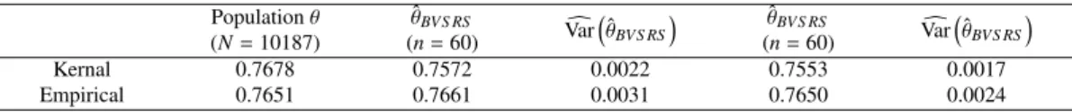
Table 3:Kernel smoothed and empirical estimates ofθ=P(X>Y) under two sampling schemes (BVSRS vs. BVRSS) Populationθ θˆBVS RS c Var(θˆBVS RS) θˆBVS RS Varc(θˆ BVS RS ) (N=10187) (n=60) (n=60) Kernal 0.7678 0.7572 0.0022 0.7553 0.0017 Empirical 0.7651 0.7661 0.0031 0.7650 0.0024
The estimates and variances are calculated based on 500 bootstrap samples.
BVRSS=bivariate ranked set sampling; BVSRS=bivariate simple random sampling.
expected that healthier individual should have larger apoA values than apoB, so they have less risk for cardiovascular disease. These apolipoproteins can be applied as alternative biomarkers to the traditional LDL and HDL biomarkers, which are sometimes more advantageous.
For example, compared to the traditional biomarker LDL-C and HDL-C, taking the
measure-ment of apoB/apoA-I ratio does not require fasting, and the measurement of apoB and apoA-I are
standardized and easy to compare across studies (Walldius and Jungner, 2006). Instead of the ratio between apoA and apoB, alternatively, we can consider the probability of apoA being greater than
apoB, where both were from the same individual (i.e.,θ=P(apoA > apoB)). If this probability is
significantly larger than 0.5, then we can say apoA is stochastically larger than apoB for the study population, thus concluding the study population is relatively at low risk of cardiovascular disease.
The data set contains apoA and apoB biomarker values taken from 10,187 Chinese children and
adults (aged≥7) in year 2009. By assuming the existing full data set as the study population, we
would want to collect a paired sub-sample of size 60 and each pair contains apoA and apoB values from the same individual. Henceforth, two sub-samples are drawn based on BVSRS and BVRSS. The kernel and empirical estimates and corresponding variances calculated by 500 resamples for
P(apoA > apoB) under the two sampling schemes are listed in Table 3. Note that the estimates of
the full data set are considered as the true value for the population parameter. For this data set, we observed that both the kernel and the empirical estimates under the two sampling schemes are very similar and are close to the true values, while BVRSS yields smaller estimated bootstrap variances.
Table 3 shows that the estimatedP(apoA>apoB) is about 0.76 which is larger than 0.5. Therefore,
we can claim that the Chinese people (aged≥7) are relatively at low risk of cardiovascular disease.
6. Final remarks and conclusions
The interest of drawing inferences aboutθ = P(X >Y) arises naturally in many areas of research,
including but not limited to the reliability for a system with strengthXand stressY, to medicine when
XandYare the outcomes of a control and an experimental treatment where, the parameterθcan be
interpreted as the effectiveness of the treatmentY, and this quantity is also related to the Receiver
Operating Characteristic (ROC) curves, whereθis interpreted as an index of accuracy. Therefore, it
is of interest to find a sampling strategy which provides more structured and representative samples
to provide more efficient and reliable estimates ofθ.
This paper shows that empirical and kernel estimates ofθ based on BVRSS and BVSRS are
equivalent in terms of bias, with both methods have small biases. As expected, bias improves as the
sample size increases. However, using BVRSS is more efficient than using BVSRS in the case of
empirical and kernel estimation. If the ranking cost of the two variables is negligible compared with that associated with taking their exact measurements, using BVRSS will result in reducing the number of subjects in the study and hence the overall cost of the study.
References
Al-Hussaini EK, Mousa MA, and Sultan KS (1997). Parametric and nonparametric simulation of
P(Y < X) for finite mixtures of lognormal components, Communications in Statistics-Theory
and Methods,26, 1269–1289.
Al-Saleh MF and Zheng G (2002). Estimation of bivariate characteristics using ranked set sampling,
Australia and New Zealand Journal of Statistics,44, 221–232.
Awad AM, Azzam MM, and Hamdan MA (1981). Some inference results on Pr(Y < X) in the
bivariate exponential model,Communications in Statistics-Theory and Methods,10, 2515–2525.
Baklizi A and Abu-Dayyeh W (2003). Shrinkage estimation ofP(Y < X) in the exponential case,
Communications in Statistics-Simulation and Computation,32, 31–42.
Baklizi A and Eidous O (2006). Nonparametric estimation ofP(X<Y) using kernel methods,Metron,
64, 47–60.
Barbiero A (2012). Interval estimators for reliability: the bivariate normal case,Journal of Applied
Statistics,39, 501–512.
Domma F and Giordano S (2012). A stress-strength model with dependent variables to measure
household financial fragility,Statistical Methods&Applications,21, 375–389.
Domma F and Giordano S (2013). A copula based approach to account for dependence in
stress-strength models,Statistical Papers,54, 807–826.
D´ıaz-Franc´es E and Montoya JA (2013). The simplicity of likelihood based inferences forP(X<Y)
and for the ratio of means in the exponential model,Statistical Papers,54, 499–522.
Enis P and Geisser S (1971). Estimation of the probability that Y < X, Journal of the American
Statistical Association,66, 162–168.
Gupta RC, Ghitany ME, and Al-Mutairi DK (2013). Estimation of reliability from a bivariate log
normal data,Journal of Statistical Computation and Simulation,83, 1068–1081.
Johnson ME (1987).Multivariate Statistical Simulation, John Wiley & Sons, New York.
Johnson NL (1975). Letter to the editor,Technometrics,17, 393.
Kaur A, Patil GP, Sinha AK, and Taillie C (1995). Ranked set sampling: an annotated bibliography,
Environmental and Ecological Statistics,2, 25–54.
Kotz S, Lumelskii S, and Pensky M (2003). The Stress-Strength Model and Its Generalizations:
Theory and Applications, World Scientific Publishing, Singapore.
Li D, Sinha BK, and Chuiv NN (1999). On estimation of P(X > c) based on a ranked set sample.
In UJ Dixit and MR Satam (Eds),Statistical Inference and Design of Experiments(pp. 47–54),
Alpha Science International, Oxford, UK.
McIntyre GA (1952). A method for unbiased selective sampling, using ranked set,Australian Journal
of Agricultural Research,3, 385–390.
Montoya JA and Rubio FJ (2014). Nonparametric inference for P(X < Y) with paired variables,
Journal of Data Science,12, 359–375.
Muttlak HA, Abu-Dayyeh WA, Saleh MF, and Al-Sawi E (2010). EstimatingP(Y<X) using ranked
set sampling in case of the exponential distribution,Communications in Statistics-Theory and
Methods,39, 1855–1868.
Nadarajah S (2005). Reliability for some bivariate beta distributions,Mathematical Problems in
En-gineering,2005, 101–111.
Norris RC, Patil GP, and Sinha AK (1995). Estimation of multiple characteristics by ranked set
sampling methods,Coenoses,10, 95–111.
Parzen E (1962). On estimation of a probability density function and mode,Annals of Mathematical
Patil GP, Sinha AK, and Taillie C (1993). Relative precision of ranked set sampling: a comparison
with the regression estimator,Environmetrics,4, 399–412.
Patil GP, Sinha AK, and Taillie C (1994). Ranked set sampling for multiple characteristics,
Interna-tional Journal of Ecology and Environmental Sciences,20, 94–109.
Patil GP, Sinha AK, and Taillie C (1999). Ranked set sampling: a bibliography,Environmental and
Ecological Statistics,6, 91–98.
Rubio FJ and Steel MFJ (2013). Bayesian inference for P(X < Y) using asymmetric dependent
distributions,Bayesian Analysis,8, 43–62.
Samawi HM, Ahmed MS, and Abu-Dayyeh W (1996). Estimating the population mean using extreme
ranked set sampling,Biometrical Journal,38, 577–586.
Samawi HM and Al-Sagheer OA (2001). On the estimation of the distribution function using extreme
and median ranked set sampling,Biometrical Journal,43, 357–373.
Samawi HM and Muttlak HA (1996). Estimation of ratio using ranked set sampling, Biometrical
Journal,38, 753–764.
Samawi HM and Muttlak HA (2001). On ratio estimation using median ranked set sampling,Journal
of Applied Statistical Science,10, 89–98.
Sengupta S and Mukhuti S (2008). Unbiased estimation ofP(X > Y) for exponential populations
using order statistics with application in ranked set sampling, Communications in
Statistics-Theory and Methods,37, 898–916.
Silverman BW (1986). Density Estimation for Statistics and Data Analysis, 26, CRC Press, New
York.
Tong H (1974). A note on the estimation of Pr(Y <X) in the exponential case,Technometrics,16,
625.
Ventura L and Racugno W (2011). Recent advances on Bayesian inference forP(X <Y),Bayesian
Analysis,6, 411–428.
Walldius G and Jungner I (2006). The apoB/apoA-I ratio: a strong, new risk factor for cardiovascular
disease and a target for lipid-lowering therapy: a review of the evidence,Journal of Internal
Medicine,259, 493–519.
Walldius G, Jungner I, Aastveit AH, Holme I, Furberg CD, and Sniderman AD (2004). The apoB/
apoA-I ratio is better than the cholesterol ratios to estimate the balance between plasma proatherogenic
and antiatherogenic lipoproteins and to predict coronary risk, Clinical Chemical Laboratory
Medicine,42, 1355–1363.
Wand MP and Jones MC (1995).Kernel Smoothing, Chapman and Hall, London.
Yan S, Li J, Li S, Zhang B, Du S, Gordon-Larsen P, Adair L, and Popkin B (2012). The
expand-ing burden of cardiometabolic risk in China: the China Health and Nutrition Survey,Obesity
Reviews,13, 810–821.
Zhou W (2008). Statistical inference forP(X<Y),Statistics in Medicine,27, 257–279.