Essays in program evaluation

(1)

2020

Essays in program evaluation

Niklaus Carlton Julius

Iowa State University

Follow this and additional works at: https://lib.dr.iastate.edu/etd

Recommended Citation Recommended Citation

Julius, Niklaus Carlton, "Essays in program evaluation" (2020). Graduate Theses and Dissertations. 17880.

https://lib.dr.iastate.edu/etd/17880

This Thesis is brought to you for free and open access by the Iowa State University Capstones, Theses and Dissertations at Iowa State University Digital Repository. It has been accepted for inclusion in Graduate Theses and Dissertations by an authorized administrator of Iowa State University Digital Repository. For more information, please contact [email protected].

(2)

by

Niklaus Carlton Julius

A dissertation submitted to the graduate faculty in partial fulfillment of the requirements for the degree of

DOCTOR OF PHILOSOPHY

Major: Economics

Program of Study Committee: Helle Bunzel, Co-major Professor Ot´avio Bartalotti, Co-major Professor

Brent Kreider Ulrike Genschel

Désiré Kédagni

The student author, whose presentation of the scholarship herein was approved by the program of study committee, is solely responsible for the content of this dissertation. The

Graduate College will ensure this dissertation is globally accessible and will not permit alterations after a degree is conferred.

Iowa State University Ames, Iowa

2020

(3)

TABLE OF CONTENTS

LIST OF TABLES . . . iv

LIST OF FIGURES . . . v

ACKNOWLEDGEMENTS . . . vi

ABSTRACT . . . vii

CHAPTER 1. A NOTE ON BOOTSTRAPS FOR MATCHING ESTIMATION . . 1

1.1 Introduction . . . 1

1.2 Setup and Notation . . . 3

1.3 Proposed Bootstrap . . . 6

1.4 Simulations . . . 9

1.5 Conclusion . . . 12

CHAPTER 2. MATCHING AS WEIGHT SELECTION: A FRAMEWORK FOR EVALUATING MATCHING ALGORITHMS . . . 15

2.2 Setup & Notation . . . 18

2.3 Optimal Weights . . . 20

2.3.1 Unconstrained Weights . . . 20

2.3.2 Constrained Weights . . . 22

2.4 Evaluating Matching Procedures . . . 24

2.4.1 ‘Augmented’ Matching . . . 24

2.4.2 Simulation Evidence . . . 25

2.4.3 Discussion . . . 30

CHAPTER 3. THE EFFECT OF TEACHER GENDER ON STUDENTS OF DIF-FERING ABILITY: EVIDENCE FROM A RANDOMIZED EXPERIMENT . . 32

3.2 Related Literature . . . 34

3.3 Data . . . 38

3.3.1 The National Evaluation of Teach for America . . . 38

(4)

3.4 Estimation Strategy . . . 42

3.4.1 The Abrevaya et al. (2015) CATE Estimator . . . 43

3.4.2 Identification Strategy . . . 43

3.4.3 Choice of Smoothing Parameters . . . 46

3.5 Results . . . 47

3.5.1 Conditioning on Pre-Treatment Test Score . . . 47

3.5.2 Conditioning on Class Rank . . . 51

3.6 Discussion . . . 53

BIBLIOGRAPHY . . . 59

APPENDIX A. ADDITIONAL MATERIAL FOR CHAPTER 1 . . . 64

APPENDIX B. ADDITIONAL MATERIAL FOR CHAPTER 2 . . . 68

(5)

LIST OF TABLES

Table 2.1 High Variance, UniformX . . . 26

Table 2.2 Low Variance, UniformX . . . 27

Table 2.3 High Variance, NormalX . . . 28

Table 2.4 Low Variance, Normal X . . . 29

Table 3.1 Descriptive Statistics . . . 57

(6)

LIST OF FIGURES

Figure 1.1 Proposed and Synthetically Corrected Bootstrap (α= 1) . . . 11

Figure 1.2 Proposed and Synthetically Corrected Bootstrap (α= 1/3) . . . 12

Figure 1.3 Proposed and Synthetically Corrected Bootstrap (α= 0.05) . . . . 13

Figure 3.1 Pre-Treatment Test Score Distribution . . . 41

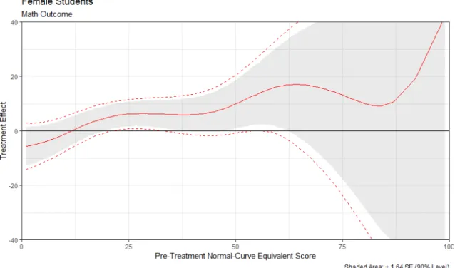
Figure 3.2 CATE (Math) for female students . . . 47

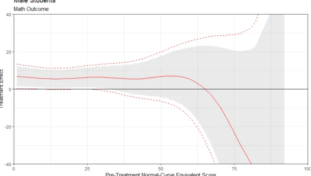
Figure 3.3 CATE (Math) for male students . . . 49

Figure 3.4 CATE (Reading) for female students . . . 51

Figure 3.5 CATE (Reading) for male students . . . 52

Figure 3.6 Conditioning on Class Rank . . . 53

Figure A.1 Proposed and Synthetically Corrected Bootstrap (ATC) . . . 67

Figure C.1 CATE Estimates (Math) with bandwidth = 0.25 . . . 76

Figure C.2 CATE Estimates (Reading) with bandwidth = 0.25 . . . 76

Figure C.3 CATE Estimates with bandwidth = 1 . . . 77

Figure C.4 CATE Estimates with bandwidth = 2 . . . 78

Figure C.5 CATE Estimates with Rectangular KernelKr . . . 82

Figure C.6 CATE Estimates with Epanechnikov kernel Ke . . . 83

Figure C.7 CATE Estimates with Teacher Certification Indicator . . . 84

Figure C.8 CATE Estimates without demographics . . . 85

Figure C.9 CATE Estimates (Math) with School Fixed Effects . . . 86

(7)

ACKNOWLEDGEMENTS

I would like to take this opportunity to thank everyone who supported me in the course of completing this work. First and foremost, my co-major professors, Dr. Helle Bunzel and Dr. Otávio Bartalotti, for their guidance, patience, and unwavering support throughout my time as a graduate student. I also thank Dr. Gray Calhoun and Dr. Brent Kreider for their invaluable advice and support in the initial stages of my graduate career. I thank my committee members, Dr. Ulrike Genschel and Dr. Désiré Kédagni, for their efforts and flexibility. Finally, I would like to thank the members of the Econometrics Reading Group for their insightful input on parts of this work.

(8)

ABSTRACT

This dissertation consists of three chapters on program evaluation, or the estimation of treatment effects.

The first chapter discusses bootstrap methods for inference on matching estimators, a popular approach to program evaluation. Abadie and Imbens (2008) showed that the standard non-parametric bootstrap fails to provide valid inference with matching estimators, and conjectured that a wild bootstrap could solve the problem. Otsu and Rai (2017) confirmed this conjecture, providing a wild bootstrap procedure that is valid in general. Their bootstrap builds in a bias correction procedure that requires estimation of conditional mean functions, a procedure that is generally necessary for consistent matching estimation. However, this step also introduces a new source of estimation error, lessening the efficiency of the bootstrap. I show that even in a special case, when bias correction in the estimator is unnecessary, the conditional mean function estimation is a required element of any wild bootstrap for the matching estimator. This shows that the Otsu and Rai bootstrap cannot be modified to be more efficient even by leveraging much stronger assumptions. Simulations provide additional support for this conclusion.

The second chapter also deals with matching estimators. I consider the problem faced by a practitioner who wishes to use matching estimation to estimate a treatment effect - in particular, choosing from a large set of available matching procedures. I cast matching esti-mators as two-step procedures - a weight-generation step followed by a weighted difference in means - and derive weights that minimize mean-squared error (MSE) under certain con-ditions. Understanding why the optimal weights behave the way they do generates insights about which matching procedures are likely to minimize MSE, enabling practitioners to use their economic intuition, knowledge of the empirical context, and knowledge of the

(9)

sam-pling process to choose an appropriate matching procedure. I develop a simple ‘augmented’ matching procedure to illustrate, and through simulation confirm that the guidance I offer is correct.

In the final chapter, I apply my program evaluation expertise to a question in the economics of education - specifically, the effect of teacher gender on student test scores. Previous literature in this vein has focused on the estimation of average effects. By exploit-ing random assignment of students to teachers in a field experiment, I study heterogeneity in the impact of teacher gender on math and reading test outcomes for primary school stu-dents of differing ability. I find that assignment to a female teacher is generally positive for male students, while it has no significant effect for female students. In addition, I find very little heterogeneity in the effect of teacher gender along the ability axis, suggesting that average effect estimates from previous investigations do not mask significant heterogeneity. My results are consistent with differential teacher behavior based on gender stereotypes, and somewhat inconsistent with differential student behavior based on gender stereotypes.

(10)

CHAPTER 1. A NOTE ON BOOTSTRAPS FOR MATCHING ESTIMATION

Matching estimators are a popular approach to program evaluation. Abadie and Im-bens (2008) showed that the naive bootstrap fails to provide valid inference with matching estimators, and conjectured that a wild bootstrap could solve the problem. Otsu and Rai (2017) confirm this conjecture. I show that even with much stronger assumptions, the Otsu and Rai (2017) bootstrap cannot be modified to be more efficient.

1.1 Introduction

Evaluating the efficacy of programs or treatments requires the estimation of treatment effects. A popular nonparametric method for estimating average treatment effects is the method of matching, which has significant intuitive appeal. These methods match treated units to control units that are ‘close’ as measured by a chosen metric. The estimated average treatment effect is then constructed by averaging the differences between matched units.

Matching can be done with or without replacement, but the latter is more common. Abadie and Imbens (2006) began a comprehensive study of matching estimators, continued in a series of papers (Abadie and Imbens, 2008, 2011, 2009, 2016). Abadie and Imbens (2006) found that matching on covariates is not always √N-consistent, generally requiring a bias correction. Abadie and Imbens (2008) showed that even when the matching estimator is √N-consistent, the ‘naive’ bootstrap1 fails to correctly estimate the distribution of the matching estimator.

1

(11)

Abadie and Imbens (2008) traced the failure of the naive bootstrap to a failure to capture the behavior of the matching process that underlies the estimator. Specifically, a given control observation will tend not to be matched to the same treated units, or even the same number of treated units, across the true and bootstrapped samples. Abadie and Imbens (2008) noted that this reasoning clearly suggests a wild bootstrap could avoid the problem, by conditioning the bootstrap on realized matches in the true sample. Otsu and Rai (2017) confirm this conjecture, providing a consistent bootstrap procedure for matching estimators that match on covariates.

Because Otsu and Rai (2017) developed a bootstrap that is valid in general, it naturally incorporates the bias correction that is sometimes required for consistency of the matching estimator. This entails the estimation of conditional mean functions for units in both treatment arms, which introduces an additional source of estimation error. It is reasonable to suspect that eliminating this estimation error might generate efficiency gains in the bootstrap, at the cost of generality.

In this chapter, I show that conditional mean estimation is necessary for a valid wild bootstrap even without bias correction. Considering a special case where matching estima-tion is consistent without bias correcestima-tion, I develop a natural wild bootstrap and show that it fails to consistently estimate the variance of the matching estimator. Potential solutions to the problem fall into two categories: those that essentially reproduce the bootstrap from Otsu and Rai (2017), and those that abandon the wild bootstrap entirely.

The remainder of the chapter is organized as follows. In Section 1.2, I introduce notation and give a formal explanation of matching estimators. In Section 1.3, I propose a wild bootstrap without bias correction, and show theoretically that it fails in general. In Section 1.4, I provide simulation evidence of the failure. Finally, in Section 1.5 I conclude by providing an intuition for the failure and some potential avenues for future research.

(12)

1.2 Setup and Notation

Suppose we observe a random sample of sizeN =N1+N0, which consists ofN1units that received treatment andN0 units that did not receive treatment. For each uniti= 1, ..., N, we observe a triplet consisting of a treatment indicatorDi ∈ {0,1}, a covariateXi, and the outcome variable Yi =DiYi(1) + (1−Di)Yi(0). Yi(1) andYi(0) are the potential outcomes for unit iwhenDi = 1 andDi= 0, respectively.

In general, Xi can be a vector of multiple covariates. In this chapter, I restrict my attention to the case where Xi is scalar, as this is a simple way to eliminate the need for bias correction. While it is possible forXito be a vector of multiple covariates and for bias correction to be unnecessary, it has no impact on my conclusions whetherXi is a scalar or vector.

Given this sample, we seek to conduct inference on the average treatment effect for the treated population2 (the ATT),

τt=E[Yi(1)−Yi(0)|Di = 1] (1.1)

To estimate τt, we use an M nearest-neighbor matching estimator of the type studied in Abadie and Imbens (2006). Matching is based on covariate distance. Formally, the estimator is described as follows:

ˆ τt= 1 N1 X i:Di=1 Yi(1)−Y[i(0) (1.2)

where_Y[_i_{(0) is an estimate of the unobserved potential outcome, defined as}

[ Yi(0) =        Yi, ifDi = 0, 1 M P j∈JM(i)Yj, ifDi= 1 (1.3)

2_{The restriction to the ATT is without loss of generality. The extension to the case of the average} treatment effect for the untreated population (the ATC) is straightforward, and extending the result to the case of the average treatment effect for the whole population (the ATE) follows from the representation of the ATE as a weighted average of the ATT and the ATC.

(13)

J_M(i) is the set of indices describing the M closest matches to unit i. Formally, it is defined as JM(i) =    j ∈ {1, ..., N}:Dj = 0, X l:Dl=0 I{|Xl−Xi |≤|Xj−Xi|} ≤M    (1.4)

As an example, suppose that for some treated unit i,Xi = 4. Suppose there are three control unitsj, k, l, withXj = 3.5,Xk = 4.6,Xl= 5. J1(i) is the closest match, and would thus be the singleton set {j}. J2(i) would be {j, k}, and J3(i) would be {j, k, l}. For the remainder of the chapter, I generally restrict attention to the case whereM = 1 - a common choice in practice, and one which eases exposition considerably.

It is useful to define Ki as the number of times unit iis used as a match

Ki =        0, ifDi= 1, P j:Dj=1I{i∈ JM(i)}, ifDi = 0 (1.5)

Let m(i) be a function that returns the single value in J_M(i) when M = 1. Finally, let

µ(d, x) =E[Y |D=d, X =x] and σ2(d, x) = Var (Y |D=d, X =x).

Abadie and Imbens (2006), in their study of matching estimators of this kind, considered the case where N grows while M remains constant. Otsu and Rai (2017) refer to this as ‘fixed-M asymptotics’. Under the following assumptions, Abadie and Imbens were able to characterize the asymptotic behavior of ˆτt.

AI.1 Conditional on Di =d, the sample consists of independent draws from Y, X |D =d for d∈ {0,1}. For somer ≤1, N₁r/N0 →θ∈(0,∞).

AI.2 X is continuously distributed on compact and convex support X⊂R. The density of

X is bounded and bounded away from zero on X.

AI.3 D is independent of Y(0) conditional on X =x for almost every x. There exists a positive constant c such that Pr[D= 1|X=x]≤1−c for almost every x.

AI.4 For d∈ {0,1}, µ(d, x) and σ2(d, x) are Lipschitz inX, and σ2(d, x) is bounded away from zero on X.

(14)

Assumptions AI.1 through AI.3 are relatively standard. They provide useful conditions on the sampling process and the distribution of X, along with the standard unconfound-edness and overlap assumptions necessary to identify the ATT. AI.4 provides smoothness and bounds that are necessary for the characterization of the bias term and its asymptotic behavior.

Under these assumptions, Abadie and Imbens (2006) showed that ˆτt→p _τt_{, and} √ N1 τˆt−BNt −τt σ_Nt → d_N₍₀_,₁₎ _(1.6) where B_Nt = N X i=1 Di   1 M X j∈JM(i) [µ(0, Xi)−µ(0, Xj)]   (σ_Nt )2 = (σ₁t_N)2+ (σ₂t)2 σt₁_N = 1 N1 N X i=1 Di+ (1−Di) 1 MKi 2 σ2(Di, Xi) (σ2₂)2 =E(µ(1, Xi)−µ(0, Xi)−τt)2|Di = 1 (1.7)

Inuitively,B_Nt captures the bias produced by matches that are less than perfect. Since se-lection on observables is contained in assumptions AI.1 through AI.4, ifXj =Xi,µ(0, Xi)−

µ(0, Xj) = 0 follows trivially. σ1tN captures the variance effect of units being matched poten-tially multiple times3. Finally, (σt₂)2 captures the variance produced by innate differences in the treatment effect conditional on X. If τt _{did not depend on} _X_{, for instance, (}_σt

2)2 would trivially be zero.

When Xi is scalar,Bt_N isop(N

−1/2

1 ) and thus asymptotically ignorable. Alternatively, I could directly restrict attention to cases whereBt_N isop(N

−1/2

1 ), which occurs whenr > k/2, effectively placing a strong restriction on the growth rate of the different treatment arms in the sampling process. Intuitively, B_Nt is ignorable when N0 grows at least as fast as

√ N1. It is more common for control groups to be at least as large as treatment groups, so for

3

Note that ifKi= 1 for alli,σt1N devoles into the average ofσ

2

(15)

the purposes of estimating the ATT this requirement is often satisfied, further supporting an exploration for a special case of the bootstrap without bias correction. When B_Nt is not ignorable, the bias term grows because the number of matches required grows faster than the ‘quality’4 of matches shrinks, resulting in the average ‘quality’ of matches decreasing as

N increases.

1.3 Proposed Bootstrap

Otsu and Rai (2017) provide a valid wild bootstrap for the general case of theM-nearest neighbor matching estimator described above, for any number of continuous covariates. In their setting,Bt_N is not guaranteed to beop(N

−1/2

1 ). Thus, as a bias correction is needed in the estimation procedure, part of the bootstrap must also account for the variance generated by the bias correction. Otsu and Rai solve this problem by simply bootstrapping the bias correction itself, which requires estimating of the conditional mean functions µ(d, x) for

d∈ {0,1}. It is reasonable to suspect that estimation errors in this step may increase the estimated variance of ˆτt_{, and thus that a bootstrap without the bias correction might be} more efficient, at the cost of being invalid when a bias correction is needed.

The reason a wild bootstrap was conjectured by Abadie and Imbens (2008) is that by definition, a wild bootstrap will not change the matches and thus will not need to estimate the distribution ofKi. I consider the following procedure:

1. Estimate ˆτt using nearest-neighbor matching.

2. Using ˆτt from step 1, generate residuals ˆξi = Yi(1)−τˆt

−_Y[_i_{(0) .}

3. Draw a bootstrap auxiliary variable ∗_i from the Rademacher distribution. 4. Create bootstrapped treated outcomes Yi(1)∗ =Y[i(0) + ˆτt+∗iξˆi.

5. Estimate ˆτt∗ _{using nearest-neighbor matching on the bootstrapped sample.}

4_{The ‘quality’ of a match can be thought of as the difference between}_µ₍_Xi,_{0) and}_µ₍_Xj,_{0) for}_i_and _j being matched together.

(16)

6. Repeat steps 1-5B times, and use the sample variance of ˆτt∗ to estimate the variance of ˆτt.

Davidson et al. (2007) provides strong evidence that the Rademacher distribution is superior for wild bootstrap performance. Indeed, their results suggest that the Rademacher distribution is one of the best distributions possible. The Rademacher distribution is very simple, with ∗_i taking the values 1 and −1 with equal probability.

This is a prima facie reasonable procedure. While it may appear odd at first for the bootstrapped dataset to consist of (Y(1)∗, Y(0)), this is a result of estimating the ATT. BootstrappingY(0) would require defining and constructing estimates of_Y[_i_{(1), which} can-not be done without estimating the average treatment effect for the whole population, or estimating conditional mean functions as in Otsu and Rai (2017). Asτt is often an object of interest in itself, a wild bootstrap for this case is worth having.

Unfortunately, the proposed bootstrap is not valid in general. Furthermore, the failure indicates that any wild bootstrap that does not construct_Y[_i_{(1) will not be valid in general.} The failure is not total - in certain special cases5, the procedure works correctly. The special cases offer an intuition for why the procedure fails in general. Solving this problem essentially requires replicating the Otsu and Rai (2017) bootstrap procedure by estimating conditional mean functions to construct_Y[_i_{(1), or abandoning the wild bootstrap altogether.} The simplest option in the latter category is to bootstrap the treatment indicator Di rather thanYi. As this approach relies on estimating propensity scores, which is done for all observations even when estimating the ATT, it avoids the incomplete bootstrapping issue. This approach is illustrated in Huber et al. (2016) and Adusumilli (2017).

For the proposed bootstrap to work, it would suffice for the following to be true,

sup q Pr np N1 τˆt∗−τˆt ≤q |Z o −PrnpN1 τˆt−τt ≤q o → p ₀ _(1.8)

5_{Most notably, in the case where each treated unit has a}_unique_{closest match in the control group, and} also in the case where treated units have zero idiosyncratic errors.

(17)

where Z= {Y, D, X} is the entire sample. Abadie and Imbens (2006) show (in Corollary 1) that√N1(ˆτt−τt)/σNt is asymptotically normal, so (1.8) implies the following:

VarpN1 τˆt∗−τˆt |Z−(σ_Nt )2→p 0 (1.9) Pr np N1 τˆt∗−τˆt /σt_N ≤t|Zo−Φ(t) → p ₀ _∀ _t_∈ R (1.10)

Intuitively, (1.9) requires that the bootstrapped estimates ˆτt∗ have the correct variance, and (1.10) requires that the bootstrapped estimates are asymptotically normally distributed. Note that either condition failing to hold is sufficient to prove that the bootstrap does not work. I will give an abbreviated proof here, as the failure is interesting.

It is possible to recover a representation for ˆτt∗ from the proposed bootstrap procedure,

ˆ τt∗ = ˆτt+ 1 N1 N X i=1 Diξˆi∗i (1.11)

This representation can be decomposed into a form involving estimated population pa-rameters and the papa-rameters themselves:

ˆ τt∗ = ˆτt+ 1 N1 N X i=1 Diξi∗i + 1 N1 N X i=1 Di ˆ ξi−ξi ∗_i = ˆτt+T_Nt∗+Qt_N∗+Rt_N∗ (1.12) where T_Nt∗ = 1 N1 N X i=1 Di µ(1, Xi)−µ(0, Xi)−τt ∗_i Qt_N∗ = 1 N1 N X i=1 Di Yi(1)−Y[i(0)−µ(1, Xi) +µ(0, Xi) ∗_i Rt_N∗ = 1 N1 N X i=1 Di τt−τˆt ∗_i (1.13)

In simple terms,T_Nt∗is a term capturing the differences between the true treatment effect at some value ofXi and the ATT.Qt_N∗ captures the variance contributed by the ‘quality’ of the matches as well as some remainder terms, andRt∗

(18)

Noting that √N1 τˆt∗−τˆt =√N1 TNt∗+QtN∗+RtN∗ , it follows that VarpN1 τˆt∗−τˆt |Z=N1E(TNt∗)2+ (Qt ∗ N)2+ (Rt ∗ N)2|Z +N1E2 TNt∗Qt ∗ N+Tt ∗ NRt ∗ N+Qt ∗ NRt ∗ N |Z (1.14)

Under assumptions A1-A4, the following results hold:

EN1(TNt∗)2 |Z →p (σ₂t)2 EN1(QtN∗)2 |Z →p (σ₁t_N)0 EN1(RNt∗)2 |Z is Op(N −1/2 1 ) E2N1 TNt∗QtN∗+TNt∗RtN∗+QtN∗RNt∗ |Z = 0 (1.15)

The full proof is relegated to Appendix A. Note that EN1(QtN∗)2 |Z

does not con-verge to (σt₁_N)2. This is the failure of the bootstrap procedure. Instead,EN1(QtN∗)2 |Z

converges to (σt 1N)0, (σ₁t_N)0 = 1 N1 N X i=1 Di+ (1−Di) 1 MKi σ2(Di, Xi) (1.16)

When contrasted with (σt₁_N)2, the term involving Ki lacks a power of two. It is easy to see from this why the bootstrap works when each treated unit has a unique matching control unit - in that case, Ki = 1 for all i, so the missing power of two has no effect and (σt₁_N)0 = (σ₁t_N)2. Due to this failure, the variance of the bootstrapped ˆτt∗’s is incorrect, and thus the bootstrap consistency condition does not hold.

1.4 Simulations

In this section, I use the data generating process from Abadie and Imbens (2008), which is described as follows:

1. The marginal distribution of X is uniform on the interval [0,1].

(19)

3. The propensity scoree(X) = Pr [D= 1|X=x] is a constant function ofα. 4. The distribution ofY(1) is degenerate, with Pr [Yi(1) =τ] = 1.

5. The conditional distribution ofY(0)|X=x is standard normal.

This DGP enabled Abadie and Imbens (2008) to find an analytic representation for both the conditional and unconditional variance of ˆτt,

Var ˆτt = 1 N1 +3 2 (N1−1)(N0+ 8/3) N1(N0+ 1)(N0+ 2) Var ˆτt|Z= 1 N2 1 N X i=1 K_i2 (1.17)

To provide evidence not merely of a failure in the bootstrap procedure, but of the exact failure identified above, I construct a synthetically corrected bootstrap estimator by calculating T_Nt∗, R_Nt∗, and (σ₁t_N)2 directly in each bootstrapped sample. The synthetically corrected bootstrap estimator is given by

ˆ

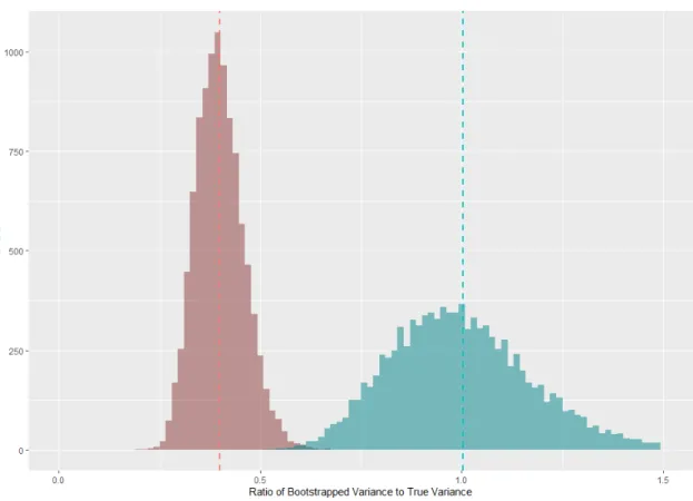
τ_st∗ = ˆτt+T_Nt∗+ (σt₁_N)2+Rt_N∗ (1.18) This estimator can be thought of as what a correct bootstrap procedure analogous to the proposed bootstrap would produce, if it were possible to correct the procedure without conditional mean estimation. All results that follow come from a 10,000-iteration Monte-Carlo simulation, withτt= 5 and 200 bootstraps per iteration.

Figure 1.1 represents a baseline case, with N = 1000 and an equal number of treated and control units. The proposed bootstrap (histogram in red) consistently underestimates the true variance of the matching estimator by a significant margin. The synthetically cor-rected bootstrap (turquoise) correctly estimates the target variance. Given the theoretical underpinnings of the failure, this is expected. The missing power in (σ₁t_N)0 will result in underestimated variance wheneverPN

i=1(Di+ (1−Di) 1 MKi)< PN i=1(DI+ (1−Di) 1 MKi)2, and this will almost always occur when the ratio of treated to control units is close to one. This logic suggests that in settings with significantly more control observations (i.e.

(20)

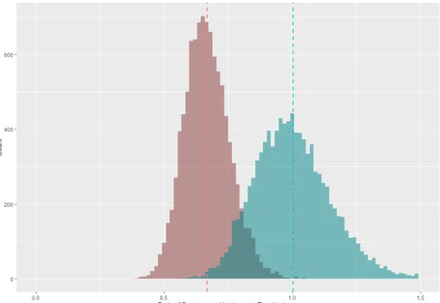
amount. This is because decreasing α causes the probability of any Ki exceeding 1 to decrease. Simulations confirm this conjecture. Figure 1.2 is the same simulation as Figure 1.1, except with 3 times as many control units for anα of 1₃.

Figure 1.1 Proposed and Synthetically Corrected Bootstrap (α= 1)

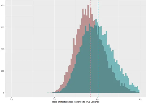
The rate at which the proposed bootstrap approaches the correct variance as α ap-proaches 0 is very slow. Figure 1.3 displays the results from a simulation withα= 0.05, and still the proposed bootstrap underestimates the target variance by a problematic amount.

In the appendix, I present simulation results for the estimation of the average treat-ment effect on the untreated population (the ATC). The Abadie and Imbens (2008) data generating process causes the failure in the proposed bootstrap to disappear due to the degenerate distribution ofY(1). With a data generating process designed to be analogous to the Abadie and Imbens (2008) process but for ATC estimation, exactly the same failure would obtain.

(21)

Figure 1.2 Proposed and Synthetically Corrected Bootstrap (α= 1/3)

1.5 Conclusion

I proposed aprima facie reasonable bootstrap for estimating the variance of the match-ing estimator of the ATT when bias correction is unnecessary. I identified a flaw in the procedure, which is not a failure to estimate the distribution of Ki as in the naive boot-strap. Instead, the failure is related to the way in which control (treated) observations contribute variance to the final estimator of the ATT (ATC). The distribution of Ki is an important component of the variance of ˆτt because it determines how important the idiosyncratic error of unit i is to that variance. The proposed bootstrap fails to correctly perturb the idiosyncratic errors of control units, leading to a consistent underestimation of the true variance.

(22)

Figure 1.3 Proposed and Synthetically Corrected Bootstrap (α= 0.05)

Otsu and Rai (2017) avoid this issue by sampling and bootstrapping two separate resid-uals. They construct these residuals by estimating the conditional mean functions µ(0, x) and µ(1, x). Avoiding the estimation errors associated with using the estimated functions ˆ

µ(0, x) and ˆµ(1, x) in the bootstrap was the was the leading source of potential improve-ments motivating this bootstrap. Thus, it appears that Otsu and Rai (2017) is currently the most efficient wild bootstrap procedure for estimating the variance of the matching estimator for treatment effects.

It is possible that a more complex bootstrap procedure may work specifically for es-timating the average treatment effect for the whole population, when bias correction is unnecessary. Otsu and Rai (2017) requires only that ˆµ(d, x) satisfies a condition on con-vergence rates, which may be satisfied by the implicit estimator ˆµ(Di, Xi) = Yi(\Di, Xi) constructed in the normal matching estimator. If so, it would be possible to perform the

(23)

Otsu and Rai (2017) bootstrap without adding an extra step to estimate ˆµ(d, x) by using the implicit estimator. However, it is unlikely that performance improvements could be gained, as estimation errors would still affect the final bootstrap results and the estimation errors associated with the implicit estimator are likely to be large compared to explicit estimators of conditional mean functions. Otsu and Rai (2017) also note that when bias correction is unnecessary, it is possible to construct a valid subsampling procedure based on Politis and Romano (1994) that does not require estimation of ˆµ(d, x), although the computational cost of this procedure is significant compared to a wild bootstrap and the procedure is sensitive to the choice of subsample size whenN is not large.

(24)

CHAPTER 2. MATCHING AS WEIGHT SELECTION: A FRAMEWORK FOR EVALUATING MATCHING ALGORITHMS

Due to non-smooth behavior of matching estimators, the bias/variance trade-offs asso-ciated with changes in the matching procedure are opaque. This leaves practitioners with limited guidance when choosing a matching procedure and its parameters. I cast matching estimators as a subset of a larger class of weighting estimators and use insights gained from considering optimal weights to offer further guidance in selection of matching procedures, selection of smoothing parameters, and potentially fruitful directions for future research.

2.1 Introduction

Matching estimation techniques have significant intuitive appeal and are relatively easy to implement. It is thus no surprise that despite Abadie and Imbens (2006) showing that they fail to reach the semi-parametric efficiency bound, they remain a popular approach to program evaluation. Perhaps due to the intuitive simplicity, a number of different ap-proaches to matching have been proposed, none of which are obviously more or less plausible than others.

Practitioners today face a choice set that includesM−nearest neighbor matching (Abadie and Imbens, 2006), caliper matching (Cochran and Rubin, 1973), radius matching (Dehejia and Wahba, 1999), coarsened exact matching (Iacus et al., 2009), matching on the propen-sity score (Rosenbaum and Rubin, 1983, 1985) and genetic matching (Diamond and Sekhon, 2013). In addition, each of these procedures requires the choice of at least one smoothing parameter (e.g. number of matches, kernel and bandwidth, degree of coarsening). King

(25)

et al. (2011) suggests that researchers should conduct an “extensive, iterative, and typically manual search across different matching solutions,” but this is unrealistically difficult to execute in practicer, and it is not clear what one should look for in this search.

In this chapter I aim to aid researchers facing this choice set by developing a framework that shrinks the relevant search space, identifying ‘directions’ within that space in which improvements are more or less likely to be found. This is accomplished by casting matching procedures as weight selectors which are followed by simple weighted difference-in-means estimation. Recasting matching estimators in this way allows me to identify infeasible optimal weights, and use the deviations from optimal weighting to generate insights about competing matching procedures.

This chapter’s main contribution is to derive weights which are optimal in the sense of reducing mean-squared error (MSE), weights that are sometimes estimable1. First, I show that in the unconstrained case optimal weights are nonzero (outside of a degenerate case). I extend the result and prove that - subject to mild regularity conditions - the MSE-optimal weights are nonzero in situations that closely approximate those that apply to weights generated by matching. Using this insight, I develop a illustrative ‘augmented’ matching algorithm and verify through simulations that it behaves as my results suggest, confirming the validity of said insights. Further, the illustrative procedure sheds light on how important it is to avoid nonzero weights as features of the data-generating process change.

Overall, my results suggest that some form of kernel matching is likely to be most promising current approach in practice, as well as the most promising approach for further development of matching procedures. This is primarily due to the flexibility inherent in kernel matching, and echoes results from Armstrong and Koles´ar (2018), who arrive at their conclusions from the consideration of worst-case MSE for weighting estimators in general.

1

However, due to the form of the optimal weight functions, the cumulative effect of estimation errors is likely to limit the gains from using estimated optimal weights.

(26)

The approach I take necessitates conditioning on the sample, which has both pros and cons2. As Armstrong and Koles´ar (2018) note, conditioning on the sample and realized treatment assignments takes into account the finite-sample possibility that imbalance may be present even with random assignment, but also precludes the use of the propensity score to gain efficiency. Like Armstrong and Koles´ar, I do not intend to argue for or against conditioning on the sample - both approaches are valuable for understanding the behavior of program evaluation estimators.

This chapter contributes to a robust literature that offers advice to researchers choosing matching procedures and smoothing parameters. One strand of this literature contributes via simulation studies which contrast different matching procedures and smoothing param-eters. For instance, Huber et al. (2013) generates data intended to replicate the features of a labor market dataset from Germany, and finds that radius matching with a regression adjustment performs best overall. Zhao (2004) considers the choice of the distance metric used in the matching procedure, a question that has received surprisingly little attention. King and Nielsen (2016) argues that propensity-score based pruning methods are inferior to other pruning methods (a claim presaged by Hahn, 1998).

Another strand of literature considers the use of weighting estimators for treatment effects more generally, without a strong focus on the connection to the method of match-ing. Most recently, Kallus (2016) and Armstrong and Koles´ar (2018) develop methods of choosing weights that minimize worst-case MSE. Armstrong and Koles´ar (2018) go on to provide asymptotically valid confidence intervals for a class ‘minimax’ optimal estimators they propose. Such ‘minimax’ estimators are designed to limit the MSE of an estimator subjected to a ‘worst-case’ data-generating process, characterized by a smoothness restric-tion on the condirestric-tional mean funcrestric-tion. Hazlett (2016) develops a method to determine which weights achieve unbiased estimation of the average treatment effect on the treated. Hainmueller (2012) proposes a weight-selection algorithm that determines weights based on

2

(27)

moment conditions selected by the researcher, and Chan et al. (2015) employs a similar approach to develop a globally efficient calibration estimator. In contrast to this chapter, this strand of literature is generally concerned with cases where there is misspecification in either the regression function or the propensity score model.

The remainder of the chapter is organized as follows. Section 2.2 introduces notation and shows how matching estimators can be represented as weight selection procedures. In Section 2.3, I derive optimal weights for unconstrained and constrained cases, prove that optimal constrained weights are nonzero subject to mild regularity conditions, and offer some intuition for why this is true. In Section 2.4, I use that intuition to develop a simple ‘augmented’ matching procedure, and contrast it’s behavior with nearest-neighbor matching and caliper matching through simulation. Finally, in Section 2.5 I conclude and suggest some directions for future research.

2.2 Setup & Notation

My notation closely follows Otsu and Rai (2017). We observe a dataset of size N, consisting of N1 units that received treatment and N0 units that did not. For each unit

i = 1, ..., N, we observe a binary treatment indicator Di, a covariate (potentially vector-valued) Xi, and an outcome,

Yi =        Yi(0) ifDi= 0, Yi(1) ifDi= 1

where Yi(1) and Yi(0) are the potential outcomes for unit i if Di = 1 and Di = 0 respec-tively. Given this sample, we seek to estimate the average treatment effect for the treated population3 (henceforth, the ATT)

τt=E[Yi(1)−Yi(0)|Di = 1]

3_{Extension of my results to the case of the average treatment effect for the untreated population (the} ATC) is straightforward. Extension to the case of the average treatment effect for the whole population (the ATE) is less so, but can most easily be recovered by noting that the ATE is a weighted average of the ATT and the ATC.

(28)

To gain traction on this estimand, it is necessary that treatment is partially uncon-founded4, that the probability of treatment assignment is bounded away from 1, and that the sample is composed of conditionally independent draws from the population distribu-tion. Formally,

A1. Dis independent of Y(0) conditional on X=x. A2. Pr [D= 1|X =x]<1−cfor some c >0.

A3. Conditional onDi =d, the sample consists of independent draws from Y, X |D=d ford∈ {0,1}.

These assumptions are standard in the matching literature. Assumptions A1 and A3 together are often referred to as ‘selection on observables’. They ensures that the potential outcomes of two observations i and j will be equal if Xi = Xj, a requirement for match-ing estimators to be asymptotically consistent. Assumption A2, often called the ’overlap’ condition, ensures that there are no portions of the covariate space in which all units are treated. If overlap does not hold, the ATT is not identified for subsets of the covariate space.

Before casting matching as a weight-selection procedure, letµ(x, d) =E[Y |X=x, D=d],

σ2(x, d) = Var (Y |X=x, D =d), and further let εi = Yi−µ(Xi, Di). Let I{A} be the indicator function that returns 1 whenAis true, and 0 otherwise. Let|x|= (x0x)1/2 be the standard Euclidean vector norm. Let JM(i) be defined as

J_M(i) =    j∈ {1, ..., N}:Dj = 1−Di, X Dl=1−Di I{|Xl−Xi| ≤ |Xj−Xi|} ≤M    (2.1)

The standard M-nearest neighbor matching estimator for the ATT is then given by

ˆ τt= 1 N1 X Di=1 Yi−Y[i(0) (2.2) 4

(29)

where [ Yi(0) =        Yi ifDi = 0, 1 M P j∈JM(i)Yj ifDi = 1

In simple terms, the M-nearest neighbor matching estimator imputes the value of _Y[_i₍₀₎ as the average outcome values of theMcontrol units with covariates closest toXi. To recast matching as a weight-selection procedure, I will make use of an alternative representation from Abadie and Imbens (2006). First, define,

KM(i) = N

X

j=1

I{i∈ JM(j)} (2.3)

KM(i) tracks the number of times that unit i is used as a match for another unit. To illustrate with a degenerate case, if N1 = 10 and N0 = 1, all 10 treated units would be matched to the single control unit. The value of KM(i) for that control unit would then be 10. Since it is more common to match with replacement, even in non-degenerate cases

KM(i) can often be larger than 1. By convention, when estimating the ATT, KM(i) = 0 when Di = 1. It is straightforward to show that (2.2) can be represented as

ˆ τt= 1 N1 X Di=1 Yi− 1 M N1 X Di=0 KM(i)Yi (2.4)

By the nature of the M-nearest neighbor matching estimator, P

Di=0KM(i) = M N1.

Lettingki =KM(i)/P_D_i₌₀KM(i), we can rewrite (2.4) as

ˆ τt= 1 N1 X Di=1 Yi− X Di=0 kiYi (2.5)

which is a weighted difference-in-means estimator.

2.3 Optimal Weights

2.3.1 Unconstrained Weights

It is natural to ask at this point what the optimal value of the vectorkiis, and minimizing MSE is a natural objective to consider. Following Abadie and Imbens (2006), I characterize

(30)

the MSE of (2.5) in a useful way. Define the sample average treatment effect on the treated (SATT): τt₍_X_{) =} 1 N1 N X i=1 (µ(1, Xi)−µ(0, Xi))

and note that the difference between ˆτt and the SATT is ˆ τt−τt₍_X_{) =} 1 N1 X Di=1 Yi− X Di=0 kiYi− 1 N1 X Di=1 µ(Xi,1) + 1 N1 X Di=1 µ(Xi,0) (2.6)

Recall that εi =Yi−µ(Xi, Di), and decompose the first term above to get ˆ τt−τt₍_X_{) =} 1 N1 X Di=1 εi− X Di=0 kiYi+ 1 N1 X Di=1 µ(Xi,0)

The error associated with ˆτt is thus ˆ τt−τ = τt₍_X₎₋_τ₊ 1 N1 X Di=1 εi− X Di=0 kiYi+ 1 N1 X Di=1 µ(Xi,0)

This offers a clear intuitive understanding of what an optimal vector of weightski would do. We cannot affect the value of

τt₍_X₎₋_τ_{through our estimation procedure - it is a} function of the sampling procedure. The role ofki is to turnPDi=0kiYiinto an estimate of

1 N1

P

Di=1µ(Xi,0), the average of the unobserved counterfactual outcomes for the treated

arm. The problem of minimizingM SEis isomorphic to the problem of setting the weighted sum of random variables to be as close as possible to some constant value. For ease of exposition, let _N1

1

P

Di=1µ(Xi,0) = µ(XD1,0). Minimizing the MSE of the estimator in

(2.5) is equivalent to solving min ki E    µ(XD1,0)− X Di=0 kiYi   2  (2.7)

The solution to this problem leads to my first result:

Theorem 1 Let σ2(Xi, Di) = σi2. If σ2i 6= σj2 in general, the weights {ki} that solve the minimization problem in (2.7) are given by:

k_i∗=µ(XD1,0)µ(Xi,0) Q j6=iσj2 PN i=1 µ(Xi,0)2Qj6=iσ2j +QN i=1σi2

(31)

All proofs are relegated to the appendix. The requirement that σ_i2 6= σ_j2 rules out the simplest form of homoskedasticity and is required to prevent the minimization problem from becoming degenerate. If σ_i2 is a non-degenerate function of the covariate vector Xi, Theorem 1 holds and the k_i∗ is at least in principle identified.

Some features of the optimal weight vector are worth noting at this point. As one would expect, if σ2_i is lower than σ2_j, k_i∗ will be larger than k∗_j if i and j have equivalent conditional means. In addition, the optimal weight vector {k∗_i} contains no zero elements unlessµ(Xi,0) = 0 for some i, orµ(XD1,0) = 0, both of which are degenerate cases.

2.3.2 Constrained Weights

Unconstrained weights are of limited use for evaluation of matching procedures, because without constraints weights can be negative and can sum to something other than 1. Neither of these outcomes is a ‘legal’ outcome of any commonly used matching procedure.

Different matching procedures have different finite-sample constraints. For instance, if one usesM nearest-neighbor matching, conditional on the sample the only weights that can be generated are integer multiples of _{M N}1

1. By way of contrast, kernel matching is capable of producing weights that lie anywhere on the interval [0,1].

However, weights that are optimal subject to sample-specific constraints are unlikely to be useful in comparisons of different matching procedures - at best, they may shed light on the trade-offs involved in the choice of smoothing parameters. These trade-offs are less opaque, so I will focus on constraints that are shared across matching procedures - in particular, that individual weights are non-negative and that the weight vector sums to 1. One can think of these as the ‘asymptotic’ constraints that obtain on matching procedures - if the sample size is unknown, these are the constraints that obtain for all matching procedures. Further refinement of the constraints is impossible without knowledge of the sample size.

(32)

Theorem 2 provides a characterization of the MSE-optimal weights, subject to the con-straint that weights are non-negative and sum to 1.

Theorem 2 The weights {k∗_i} that solve the minimization problem in (2.7), subject to

ki>0 ∀iand PN_i₌₁ki= 1, are given by:

k_ic∗ = 1−Y1PN_i₌₁0 _σY2i i +PN0 i=1 Y2 i σ2 i +µ(XD1,0) Y1PN_i₌₁0 _σ12 i −PN0 i=1 Yi σ2 i σ_i2 PN0 i=1 σ12 i + PN0 i=1 Y2 i σ2 i PN0 i=1 σ12 i −PN0 i=1 Yi σ2 i 2 + PN0 i=1 σ12 i Y1PNi=10 σ12 i −PN0 i=1 Yi σ2 i σ2₁(Y1−Yi) σ2_i (2.8)

Unfortunately, the form of kc_i∗ is not illuminating - it is, for instance, not at all clear what guarantees that k_ic∗ is non-zero. In order to derive a strict positivity result for kc_i∗, I require an additional assumption:

A4. µ(XD1,0) lies strictly between mini[µ(Xi,0)|Di = 0]and maxi[µ(Xi,0|Di = 0)]. This assumption, while it appears quite restrictive, is rather general. It can be thought of as a finite-sample analog to the overlap condition A2. In most cases, if A4 is violated it is likely that AI.2 is violated as well. However, it is possible that A4 is violated without violating A2 in very small samples, or with extremely large values ofσ_i2. In either case, if A4 is violated, matching estimation will likely perform poorly with any matching procedure.

With this additional assumption, a strict positivity result for {kc∗

i }can be proven, Lemma 1 Given assumptions A1 through A4, the MSE-optimal weight vector {k_ic∗} con-tains no zero elements.

I again relegate the full proof of Lemma 1 to the appendix. In simple terms, the proof works by showing that a vector containing a zero element can always be modified in a way that both removes the zero element and strictly reduces MSE - similar to how proofs related to Nash Equilibria search for profitable deviations.

The reason Lemma 1 is true relates to the shape of the function that describes the change in MSE when weight is ‘shifted’ from one observation to another. This function is

(33)

strictly concave and is always strictly increasing in a neighborhood around a zero ‘shift’, for appropriately selected observations. Intuitively, the ‘change in MSE function’ has this shape because the variance of the resulting estimator increases as a function of thesquared weight on observations, while the bias increases as a function of the weight itself. The MSE-optimal weight vector never generates an unbiased estimate of the ATT - as one would expect, it achieves the minimal MSE by making ‘profitable’ trade-offs between bias and variance until no such trade-off remains.

2.4 Evaluating Matching Procedures

2.4.1 ‘Augmented’ Matching

Lemma 1 is an interesting result from the perspective of one seeking to evaluate matching procedures. To the best of my knowledge, no commonly used matching procedure is designed to lower the chances of zero elements in the weight vector. Indeed, in some common settings many matching procedures will generate a wealth of zeros in the weight vector. However, the proof of Lemma 1 makes clear that the optimal weights, while nonzero, are nonetheless vanishingly small when the ‘quality’ of a match5 is poor. If one is doing nearest-neighbor matching withM = 1, it is entirely possible that zero weights are closer to optimal than the lowest positive weight that can be assigned. Nonetheless, Lemma 1 suggests that we should consider more carefully the situations that can cause zero weights, and consider whether those weights should truly be zero.

A less obvious insight from Lemma 1 is that units with similar conditional means and similar variances should receive similar weights. It is this insight which guides the ‘aug-mented’ matching algorithm proposed below. The algorithm below is to estimate the ATT, but the extension to other estimands is immediate.

5

In contrast to Chapter 1, I refer here to ‘quality’ in the sense of how farµ(Xi,0) is fromµ(XD1,0), not

(34)

‘Augmented’ Matching for the ATT

1. Perform standard nearest-neighbor matching with M = 1.

2. For each treated unit i, define a distance ri =|Xi−Xm(i)|+δ, where m(i) returns the index of the matched control unit from step 1.

3. Search for control units whose covariates lie within a ball of radius ri around Xi. If such control units exist, assign them as matches for unitias well.

4. Use the resulting matches and weight vector to estimate τt.

This procedure encapsulates nearest-neighbor matching as a special case (if δ is set to zero, it is numerically identical to nearest-neighbor matching with M = 1). The idea is that, having already matchedXi toXm(i), it is likely that units some smallδ further away are good enough matches to generate a variance decrease that outweighs the bias increase that comes from making a worse match.

To be clear, I am not advancing this procedure as the best that can be done given these insights. Rather, it is to illustrate that the insights derived are valid, and that this framework for evaluating matching procedures works. As I will show with simulations, this augmented matching procedure is too simple, but it serves to refine the insights derived so far.

2.4.2 Simulation Evidence

For my simulations, I designed a data-generating process that allows for a number of modifications that shed light on the relative performance of nearest-neighbor and augmented matching. The basic framework is quite simple - the outcome variableYi is constructed as

Yi = Xi+Diτ(Xi) +εi. I vary the distribution of Xi and εi across simulations. τ(Xi) is defined as τ(Xi) = I{Xi ≥ 0} Xi+ 2Xi2−0.4Xi3

, to generate a conditional average treatment effect function with significant heterogeneity.

(35)

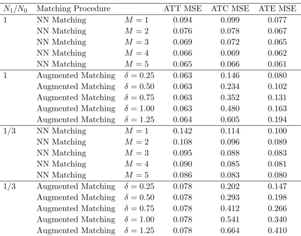
First, I draw Xi from a uniform distribution between 0 and 6. For each unit i, I also draw σ2_i from a uniform distribution between 2 and 5, and then draw εi from a meanzero normal distribution with appropriate variance. I consider two matching procedures -nearest-neighbor matching withM neighbors and augmented matching as described above. I consider five different values of M and δ. Finally, I consider two cases for the sample -one with 500 units in each treatment arm, and -one with 250 treated units and 750 control units. Table 2.1 presents the results, with 1000 simulations in each row.

Table 2.1 High Variance, UniformX

N1/N0 Matching Procedure ATT MSE ATC MSE ATE MSE 1 NN Matching M = 1 0.094 0.099 0.077 NN Matching M = 2 0.076 0.078 0.067 NN Matching M = 3 0.069 0.072 0.065 NN Matching M = 4 0.066 0.069 0.062 NN Matching M = 5 0.065 0.066 0.061 1 Augmented Matching δ = 0.25 0.063 0.146 0.080 Augmented Matching δ = 0.50 0.063 0.234 0.102 Augmented Matching δ = 0.75 0.063 0.352 0.131 Augmented Matching δ = 1.00 0.063 0.480 0.163 Augmented Matching δ = 1.25 0.064 0.605 0.194 1/3 NN Matching M = 1 0.142 0.114 0.100 NN Matching M = 2 0.108 0.096 0.089 NN Matching M = 3 0.095 0.088 0.083 NN Matching M = 4 0.090 0.085 0.081 NN Matching M = 5 0.086 0.083 0.080 1/3 Augmented Matching δ = 0.25 0.078 0.202 0.147 Augmented Matching δ = 0.50 0.078 0.293 0.198 Augmented Matching δ = 0.75 0.078 0.412 0.266 Augmented Matching δ = 1.00 0.078 0.541 0.340 Augmented Matching δ = 1.25 0.078 0.664 0.410

When estimating the ATT, the ‘quality’ of a match is simply |Xi−Xm(i)|, while for the ATC the ‘quality’ is |τ(Xi)−τ(Xm(i))|. With this data generating process, the latter grows dramatically faster than the former with the difference between Xi and Xm(i). This explains the relatively poor performance of augmented matching in the ATC case.

(36)

The ATT case makes clear that the idea of augmented matching works in some settings. Note that even with M = 5, augmented matching outperforms nearest-neighbor matching with any tested value of δ. This illustrates the chief advantages of augmented matching over changing M - it allows for a different number of matches to be found for any given unit, and has a large ‘sweet spot’ for values ofδ when match ‘quality’ is relatively flat.

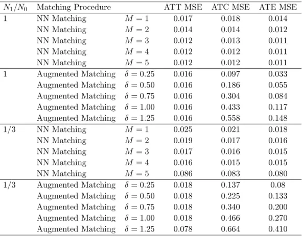
In a second simulation, I change the distribution ofσ_i2to a uniform distribution between 1 and 2, significantly restricting the potential size of idiosyncratic errors. Otherwise, the data-generating process was unchanged. Table 2.2 reports the results.

Lowering the size of idiosyncratic errors on observations would be expected to reduce the relative importance of variance in determining total MSE. Thus, one would expect augmented matching to perform more poorly relative to nearest neighbor matching in this simulation, and that is precisely what is observed.

Table 2.2 Low Variance, Uniform X

(37)

One potential issue with the augmented matching algorithm is that δ is fixed for all units. In practice, if the distribution of observations within the covariate space diverges significantly from a uniform distribution, this may cause augmented matching to perform quite poorly. In particular, in areas of the covariate space where observations are sparse, augmented matching is likely to make a small number of additional matches, and those additional matches are likely to be poor quality.

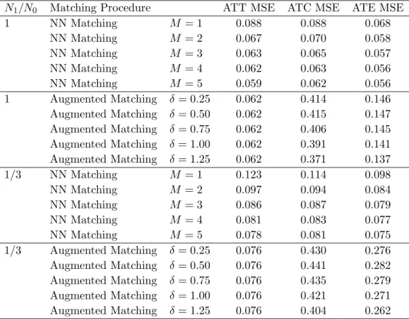
To investigate this possibility, in Table 2.3 I change the data-generating process, draw-ing Xi from a N(0,2) distribution. This generates a large mass of units around 0, with significantly fewer units available as one moves away from 0. I return to the high-variance case in terms of idiosyncratic errors, drawingσ2_i from aU[2,5] distribution.

Table 2.3 High Variance, NormalX

(38)

Somewhat surprisingly, the story is largely unchanged from the previous simulations. The relative comparison between nearest neighbor matching and augmented matching is similar to before, and nearest neighbor matching is not noticeably outperforming relative to when covariates were distributed uniformly.

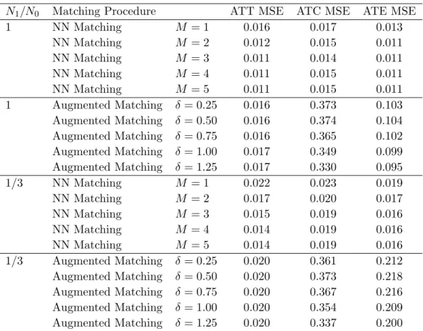
For thoroughness, Table 2.4 reports results from a final simulation that draws σ_i2 from a U[1,2] distribution.

Table 2.4 Low Variance, Normal X

It is interesting to note that when X is distributed normally, augmented matching performs better in the ATC case as δ increases - a reversal of the behavior observed when

X was distributed uniformly. However, it is clear that augmented matching in this form is not an appropriate technique for the estimation of the ATC, due to the relatively higher importance of bias in that case.

(39)

2.4.3 Discussion

A clear implication of the simulation results is that the correct δ is different when estimating the ATT and the ATC. Given the significant similarities between augmented matching, radius matching, and kernel matching, it is likely that this is true for the latter procedures as well. To the best of my knowledge, choosing the bandwidth separately for the ATT and ATC is not a common approach in practice. Since the ATE is a weighted average of the ATT and ATC, such a proposal is likely worth serious investigation, but it is beyond the scope of this investigation.

The simulations make clear that the insights derived from considering the MSE-minimizing weight vector are valid. In particular, practitioners should use economic intuition and knowl-edge of the empirical context (where possible) to weigh the relative importance of idiosyn-cratic errors and bias in the sample. In settings where bias is likely to be of low importance (for instance, if it is likely that the treatment effect is constant acrossXand the parameter of interest is the ATT), it is more likely that MSE can be reduced by matching to multiple units, or using procedures like radius and kernel matching which have strong similarities to the ‘augmented’ matching studied here. The same conclusion holds when there are many more observations in the ‘donor pool’ than in the pool of units to be matched (e.g. when estimating the ATT with many more control units than treated units).

2.5 Conclusion

Taking an approach similar to that of Armstrong and Koles´ar (2018) and Kallus (2016), I derived unconstrained MSE-minimizing weights, and MSE-minimizing weights subject to constraints that approximate those implied by many common matching procedures. Subject to a mild condition on covariate balance, MSE-minimizing weights are nonzero, and units with similar conditional means receive similar weights.

I use an illustrative, and very simple, ‘augmented’ matching procedure that builds in behavior meant to generate weights that are closer to MSE-optimal, and contrast it with

(40)

nearest neighbor matching in a variety of settings. I find that the ‘augmented’ procedure compares favorably to nearest-neighbor matching when idiosyncratic errors are an important driver of MSE, while significantly under-performing when bias is relatively more important. While the ‘augmented’ matching procedure itself is unsuitable for practical use in its current form, it confirms the insights I derive from the contrast between MSE-minimizing weights and weights from nearest neighbor matching. Practitioners can generate potentially significant reductions in MSE by carefully considering what they can reasonably determine about the data generating process, whether from economic intuition, knowledge of the empirical context, or knowledge of the data gathering process. In particular, my results suggest that defaulting to M nearest neighbor matching with M = 1 is likely to leave efficiency gains on the table in many common settings, but is a good conservative approach. This echoes Armstrong and Koles´ar (2018), who note that when the data generating process is sufficiently ‘bad’, the minimax optimal estimator is nearest neighbor matching with one match.

Further development of the ‘augmented’ matching procedure may be worthwhile. In particular, the implication that the optimal δ differs when estimating the ATT and the ATC offers a potential route to cure the under-performance observed when bias is important, through a data-driven selection ofδ. It is worth investigating whether this extends to radius and kernel matching procedures as well.

(41)

CHAPTER 3. THE EFFECT OF TEACHER GENDER ON STUDENTS OF DIFFERING ABILITY: EVIDENCE FROM A

RANDOMIZED EXPERIMENT

Gender dynamics may play an important role in the determination of student outcomes in education. Exploiting random assignment of students to teachers in a field experiment, I study heterogeneity in the impact of teacher gender on the math and reading test scores for primary school students of differing ability. I find that assignment to a female teacher is generally positive for male students while having no significant effect for female students. In addition, I find very little heterogeneity in the effect of teacher gender on the ability axis, suggesting that average effect estimates do not mask significant heterogeneity. My results are consistent with differential teacher behavior based on gender stereotypes, and somewhat inconsistent with differential student behavior based on gender stereotypes.

3.1 Introduction

Achievement on school tests has important implications for students in both the short and the long run. In the short run, test scores serve as signals to students about their ability and induce students to choose different educational paths (Mechtenberg, 2009; Lavy, 2008; Lavy and Sand, 2018; Terrier, 2016). In the long run, these choices have major implications for lifetime earnings and health outcomes (Joensen and Nielsen, 2016; Autor and Wasserman, 2013; Krueger, 2017). Gender dynamics between students and teachers can play a significant role in determining student test score outcomes (Dee, 2005; Lavy, 2008; Antecol et al., 2015; Terrier, 2016).

(42)

To date, the study of gender dynamics in the classroom has mostly considered average effects, which can mask significant heterogeneity (Bitler et al., 2006). It is possible that the effect of teacher gender on students might depend significantly on student ability, which would have important implications for policy - particularly with regard to addressing in-equality. For instance, male and female teachers may internalize different gender stereotypes and thus react differently to low- or high-performing male or female students (Williams and Ceci, 2015), or students may internalize different gender stereotypes and thus be more or less receptive to teaching from teachers of a particular gender (Ouazad and Page, 2012).

In this chapter, I address this question by studying how the effect of assignment to a female teacher changes with both the gender and ability of a student, using data from a field experiment conducted to evaluate the Teach for America (TFA) Program. I estimate the Conditional Average Treatment Effect (CATE) of assignment to a female teacher, con-ditioning on student gender and on pre-treatment test score as a proxy for ability. The CATE parameter is ideal for this study because it is a policy-relevant parameter that di-rectly addresses the question of how student ability changes the effect of teacher gender on student outcomes. My estimates show how the effect of being assigned to a female teacher changes with both student gender and student ability.

Exploiting random assignment of students to teachers in the data allows me to deploy non-parametric techniques that require the strong assumption of unconfoundedness rather than imposing functional form restrictions. While the data is not representative of the U.S. primary school student population overall, it is representative of the most disadvantaged students and schools - a subset of particular importance to policymakers. Students in these schools are less likely to continue on to higher education, and thus more likely to face the challenges facing individuals without a college education in modern society1.

1

Men with less than a four-year college education have seen a dramatic reduction in real income over the last decade (Autor and Wasserman, 2013), are less likely to enter the labor force (Krueger, 2017), and face increased risk of poverty, physical health problems, and mental health problems. The prospects for women with less than a four-year college education are significantly worse than for women with more education, but are less grim than those for men.

(43)

I find very limited heterogeneity in the effect of teacher gender on students with different levels of prior achievement. For male students, assignment to a female teacher has a nearly uniform positive impact on math test scores. In reading, there is a small positive relationship between student ability and the effect of assignment to a female teacher. For female students, there is notably more heterogeneity in the effect of teacher gender. In math, there is a stronger positive relationship between ability and the effect of teacher gender than for male students, and some indication that the lowest-performing female students might be harmed by assignment to a female teacher. In reading, there is a non-monotonic relationship between student ability and the effect of teacher gender.

My results echo much of the previous economics literature in finding no significant average effect of teacher gender on students. Outside of the bottom of the pre-treatment test score distribution, the effect of assignment to a female teacher does not significantly differ with student gender. At the very bottom of that distribution, female students may benefit less than male students from assignment to female teachers in math. Notably, for all students, the effect of assignment to a female teacher is either positive or insignificant, which suggests that biases such as those found by Lavy (2008), Terrier (2016), or Cappelen et al. (2019) are not present in primary school.

The remainder of this chapter is organized as follows. Section 3.2 reviews related lit-erature. Section 3.3 discusses the data, the institutional background, and the experiment itself. Section 3.4 briefly introduces the theoretical framework for the CATE estimator and sets out my estimation strategy. Section 3.5 presents the main results. Section 3.6 considers possible mechanisms and policy implications. Finally, Section 3.7 concludes.

3.2 Related Literature

In this chapter I contribute directly to the literature that studies student/teacher dy-namics based on demographic features, and indirectly to a related strand of literature that considers the underlying mechanisms.

(44)

Reduced form estimates of the effect of demographic matching between students and teachers go back to Ehrenberg et al. (1995), who found that demographic matching had little impact on student learning, but a significant impact on teacher perceptions of stu-dents, using NELS:882 data. Dee (2004) used Project STAR data to investigate the effect of teacher race on students, finding a positive effect of same-race teachers on math and reading for students. Dee (2005) exploited a unique feature of the NELS:88 data to control for stu-dent fixed effects, again finding that stustu-dent/teacher demographic dynamics had significant effects on teacher perceptions. Dee (2007), restricting attention to gender dynamics, found that assignment to a same-gender teacher significantly improved student test scores, teacher perceptions of the student, and student engagement.

Tertiary education has also received significant attention. Bettinger and Long (2005) and Hoffmann and Oreopoulos (2009) studied the effect of instructor gender on undergraduate students using administrative data from different universities3. Hoffmann and Oreopoulos (2009) found that assignment to a same-sex instructor boosted relative student performance and likelihood of course completion, but had little impact on upper-year course selection. Bettinger and Long (2005) found very mixed results - their primary conclusion is that the effect of instructor gender changes dramatically based on the subject in question. For instance, they found strong positive effects on female students in math and statistics, and a weak effect in economics. They also add to the growing number of studies that find negligible effects of instructor gender on male students.

Carrell et al. (2010), exploiting random assignment of students to teachers at the U.S. Air Force Academy, found limited impacts of instructor gender on male students, but sig-nificant positive impacts on female students in math and science. In contrast to Hoffmann and Oreopoulos (2009), Carrell et al. (2010) finds significant impacts for upper-year course selection. Fairlie et al. (2014), using administrative data from a community college, found 2_{The National Educational Longitudinal Study of 1988 consists of a representative sample of students} that were in 8th grade in 1988.

3

Bettinger and Long (2005) uses data on full-time undergraduate students in Ohio during 1998 and 1999. Hoffmann and Oreopoulos (2009) uses data on students at the University of Toronto.