Human Activity Tracking from Moving Camera Stereo Data

Human Activity Tracking from Moving Camera

Stereo Data

John Darby, Baihua Li and Nicholas Costen

Department of Computing and Mathematics

Manchester Metropolitan University, John Dalton Building

Chester Street, Manchester, M1 5GD, UK.

{j.darby,b.li,n.costen}@mmu.ac.uk

Abstract

We present a method for tracking human activity using observations from a moving narrow-baseline stereo camera. Range data are computed from the disparity between stereo image pairs. We propose a novel technique for calculating weighting scores from range data given body configuration hy-potheses. We use a modified Annealed Particle Filter to recover the opti-mal tracking candidate from a low dimensional latent space computed from motion capture data and constrained by an activity model. We evaluate the method on synthetic data and on a walking sequence recorded using a moving hand-held stereo camera.

1

Introduction

Annealed Particle Filtering (APF) has been shown to recover 3D human motion con-sistently using observations from 3 or more cameras [5, 7]. Silhouettes are used in the calculation of agreement between image evidence and body configuration hypotheses, or weighting function. Background subtraction is difficult to achieve without a well con-trolled experimental environment where backgrounds and sensor position are stationary. Using fewer than 3 cameras, where standard APF tracking fails rapidly [5], statistical models of human activity have been successfully used to constrain the search problem [14, 15, 17]. Offline estimation of joint locations using a 2D image-based tracker [16, 17] or assumptions about known backgrounds for silhouette extraction [11, 15] are common and the robustness to changing illumination, backgrounds, subject appearance and sensor position is limited.

A narrow-baseline stereo camera provides synchronised image pairs of a scene from 2 close-mounted parallel cameras. Processed as part of a multi-camera wide-baseline tracking scheme [7] the observations are so similar that their combination offers negligible benefit over monocular tracking performance. However, by calculation of the disparity between the paired images, range information for objects in the scene can be estimated at video frame rates [10]. In general, stereo range data provides a noisy image cue. Range accuracy is affected by errors in camera alignment and calibration while range resolution – the minimum discernable change in distance – increases as the square of the range. The issue of accuracy has led some approaches to human motion tracking to exclude stereo

range data from their calculation of hypothesis weightings [4]. We propose an activity-supervised APF method, summarised in Figure 1, to achieve robust tracking from range data. We will argue that when incorporated with an activity model, the stereo range data alone is sufficiently rich for tracking using a particle filtering approach.

Motivated by the use of chamfer images to calculate weightings from edge features in the APF algorithm [7], we introduce a chamfer volume method to compute weightings from surface features. We discretise 2.5D surface range data before smoothing it with a 3D Gaussian kernel (Section 3.3). The result is a chamfer volume where each voxel’s magnitude is proportional to its distance to a surface. We use a modified APF scheme to search for the optimum body configuration at each frame, based on comparisons between the visible surfaces of a simple body model and the chamfer volume (Section 3.2). Body configuration hypotheses are drawn from a low dimensional activity subspace recovered from motion capture (MoCap) data by Principal Components Analysis (PCA). The activ-ity space is constrained by training a hidden Markov model (Sections 3.1) which provides a model of activity dynamics and prohibits the sampling of illegal pose regions. The approach retains the reduced computational expense of PCA over nonlinear techniques (Section 2) and we hope to extend it to consider multiple activity models in multiple activity spaces in future work (Section 5). We test the proposed tracking approach using synthetic data and a sequence featuring a walking subject recorded by a moving hand-held stereo camera (Section 4).

2

Related Work

In the general case – tracking human motion where sensor evidence is weak – there have been many contributions based on the use of prior models of human behaviour. A common application is human motion tracking from monocular sequences where available image evidence is particularly ambiguous. Linear dimensionality reduction techniques such as PCA have been applied to activity training data to impose feature space constraints in the search for an optimum tracking candidate [14, 18]. Invertible nonlinear dimensionality reduction techniques such as Locally Linear Coordination (LLC) and the Gaussian Pro-cess Latent Variable Model (GPLVM) have been shown to recover rich low dimensional pose spaces from which a mapping back to the original feature space is available [11, 17]. None of PCA, LLC or GPLVM are dynamical models, and further steps must be taken to model temporal relationships in the data. For example, Hou et al. capture dynamics at different temporal scales by learning a Variable Length Markov Model from clusters in the latent space [8]. The Gaussian Process Dynamical Model [19] represents a combined approach, recovering a nonlinear low dimensional latent space and model of temporal dynamics within a single learning algorithm [16, 13].

Several approaches have incorporated stereo range data into the human motion track-ing problem. The Iterative Closest Point algorithm (ICP) was used by Demirdjian to find the transformation between a set of 3D points on a body model and a set of range data co-ordinates [6]. Articulated body model constraints were modelled by the projection of the unconstrained body model transformation onto a linear articulated motion space. Azad et al. [3] considered other image cues in addition to range data, segmenting the hands and head of the subject by colour and locating their corresponding 3D positions in range evidence. The result was used to constrain the feature space explored by a particle filter

which incorporated edge and region information into its weighting calculation. Both ap-proaches used relatively simple body models composed of rigid primitives for limbs and were shown to track sequences of upper body movement featuring some self occlusion.

Jojic et al. [9] used a body model described by an articulated set of 3D Gaussian ‘blobs’. Tracking was performed using Expectation-Maximisation and articulated con-straints enforced by an Extended Kalman Filter. Real time tracking of head and arm movements was demonstrated on a sequence featuring some self-occlusion. Pl¨ankers and Fua employed a sophisticated deformable body model to track using range and silhouette data estimated from a trinocular video sequence [12]. A set of Gaussian density distribu-tions, or ‘metaballs’ were used to form an Articulated Soft Object Model (ASOM). The form of the ASOM allows for the definition of a distance function to range data that is differentiable and so the weighting function may be maximised using deterministic op-timisation methods. The parameters of the ASOM were estimated in a frame-to-frame tracking stage by minimisation of the objective function given range data, before being refined by a global optimisation over all frames. Remarkable upper body tracking results were demonstrated on sequences of a bare-skinned subject performing abrupt arm waving and featuring self occlusion. ASOMs were later used for comparison with stereo range data featuring walking and running [18]. Full body tracking was achieved by minimising the objective function with respect to the first 5 coefficients of a pre-computed activity space recovered from MoCap training data using PCA.

3

Formulation

Parameters Particle Re-sampling Annealing & Rescaling Particle Evaluation Discretisation & Smoothing Chamfer Volume Range Data

Acquisition Final Layer N Y

Initialisation

Image Evidence Modified Annealed Particle Filter

Offline Training Particle Dispersion Expected Pose Gaussian Estimation

Figure 1: Activity-supervised APF for range image tracking.

3.1

Modelling Activity

Our body model comprises a kinematic tree with 10 truncated cones described by a 31-parameters body vector representing the torso position and orientation and the pose via relative joint angles between limbs. These body parameters can be recovered from accu-rate MoCap and we usem= 1, ..., M walking body vectors [5] to construct our activity

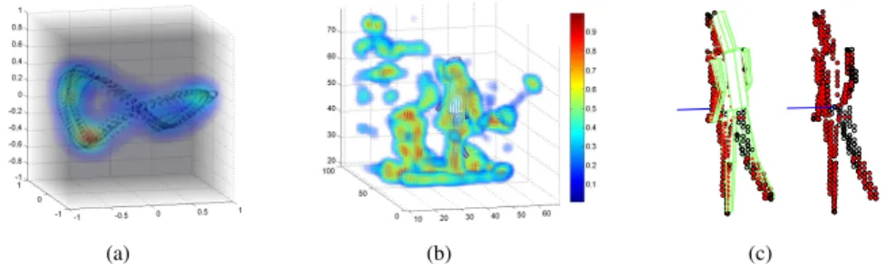
(a) (b) (c)

Figure 2: Activity model, chamfer volume and body model. (a) Latent walking data and resulting HMM observation densities; (b) Chamfer volume and body model hypothesis; (c) Rotated body model showing the extracted sample coordinates and effects of intra-and inter-cone occlusion.

model. We downsample to 30fps and remove the 9 parameters of each body vector de-scribing the torso and head,0m, as we do not want a subject’s route or line of sight to form part of the generic activity class. PCA is performed on the sequence of remaining 22D limb parameter vectorsE={1, ...,M}. By retaining the eigenvectors correspond-ing to the 4 largest eigenvaluesΦ = (φ1|...|φ4), we preserve 93% of the variance. The

data can then be approximated by the sequence of weighting vectorsF = {f1, ...,fM} usingm≈¯+Φfm. Figure 2(a) shows the body configuration trajectory projected onto the 3 highest variance eigenvectors. The full feature vector is 13D, comprising the 9 torso and head parameters and the approximation of the remaining limb parameters given by the 4D weighting vector,xm= (0m,fm).

A hidden Markov model (HMM) can be used to model a time series of observations such asF = {f1, ...,fM} where the sequence of observations is the result of a doubly stochastic process. An HMMλis specified by the parameters S,Aij,Ai,pi(f), where

S = {s1, ..., sN} is the set of states; theN ×N matrixAij gives the probability of a

transition from stateito statej;Aigives the probability of a sequence starting in statei andpi(f)is the probability of observing feature vectorfwhile in statei. We model each observation density by a single multivariate Gaussianpi(f) = N(f|µi,Σi)with mean

µi and covariance Σi. HMM training is performed using the Baum-Welch algorithm with initial estimates forµiandΣifound by k-means clustering,Aijrandomised andAi held constant as a flat distribution. Figure 2(a) shows a visualisation of the observation densities recovered by training a 15 state HMM on walking dataF.

3.2

Temporal Dynamics for APF

If human motion is recorded using a stereo camera then by assuming that the set of obser-vationsZm= (z1, ...,zm)are independent and that the evolution of the body’s configu-ration is a first order Markov process, the state density may propagated using

p(xm|Zm)∝p(zm|xm)

Z

xm−1

p(xm|xm−1)p(xm−1|Zm−1). (1)

SIR [2] allows for the representation of a multimodal posterior,p(xm|Zm), with a set of normalised, weighted particles,{(x(1)m, π

(1) m ), ...,(x (B) m , π (B) m )}.Dispersionby a model of

Initialisation:{(x(₁b),1/B)}B b=1. form= 1toMdo forr=Rdownto1do 1. Calculate weightsπm(b)=wrm(zm,x (b) m).

2. ResampleBparticles with likelihood∝π(mb)and with replacement. 3. Find most likely parent state of limb parameters:arg maxi(pi(f

(b)

m )). 4. Rescale dispersion parametersPr,Σr

i andρrT byαr. 5. MakeK_ir=lln(1−ρrT)

ln(Aii)

m

state transitions viaAijand emit an observable:

ifj6=ithen fm(b)=pj(f) =N(f|µj,Σrj). else fm(b)=p0i(f) =N(f|µ=f (b) m,Σri). end if

6. Disperse head and torso parameters0m=N(0|0(mb),Pr). 7. Concatenate to give new particle locationx(mb)= (0

(b)

m,f

(b)

m ).

end for

Calculate expected configuration for visualisationE(xm) =P B b=1π (b) mx (b) m. end for

Figure 3: Pseudocode for particle dispersion.

temporal dynamics (usually drift-and-spread),evaluationby a weighting function

w(zm,x

(b)

m) ≈ p(zm|x

(b)

m) andresamplingwith probability proportional to weighting scoreπm(b), propagates the posterior approximation over time.

APF [7] has been shown to give increased tracking accuracy [5] by cooling the weight-ing distribution and then gradually introducweight-ing sharp peaks overr=R, R−1, ...,1 sep-arate resampling layers at each time stepm:

w_mr(zm,xm) =w(zm,xm)β r m_{, β}1 m> β 2 m> ... > β R m. (2)

The value ofβ_mr is chosen to control the particle survival rateαr, the proportion of parti-cles that will be resampled. The aim of APF is to recover the hypothesis that maximises the weighting function, generally leading to a concentration of particles into a particular mode of the distribution. The posterior distribution is not fully represented, leading to a reduction in weighting function evaluations at the expense of a departure from the formal Bayesian framework.

Rather than using drift-and-spread dynamics [4] or adding noise [15] we appeal to the pre-trained activity HMM to disperse the weighting vector parameters, findingfm|fm−1

and therefore the limb parametersm. The annealing process can cause APF to recover the wrong interpretation when faced with multiple maxima of approximately equal mag-nitude in the posterior [5]. Similarly, high densities of samples in a relatively flat posterior may cause the particle set to ‘stall’. Where there are considerably fewer HMM states than training data per activity cycle, each state has a high probability of undergoing a self-transition. This is a concern during periods of particularly ambiguous image evidence, with samples likely to build up around an HMM state-mean. In anticipation we introduce a temperature parameter into the synthesis process, requiring a non-self state transition

from stateiwith some minimum probabilityρT by makingKistate transitions. In gen-eral, hypotheses that extend too far along the activity cycle die out during annealing, dis-counted by comparison with image evidence in the evaluation ofw(zm,xm). However, where image evidence becomes weak, the approach is able to maintain a wider distribu-tion of activity pose samples and escape becoming ‘stuck’ in an incorrect interpretadistribu-tion.

The remaining torso and head parameters are dispersed by the addition of Gaus-sian noise with diagonal covariance matrixPestimated from the training data to give

0m|0m−1. The covariance matrix is multiplied by the particle survival rateαrat each

annealing layer to givePr, the application of noise decreasing at the same rate as the reso-lution of the particle set increases [7]. We extend the scaling procedure to the observation densities at each HMM statepi(f) =N(f|µi,Σi)and to the transition temperatureρT, rescaling byαrat each annealing layer to giveΣr_i andρr_T (orK_irtransitions).

As the state means µi are constant, the effect of rescaling the observation densi-ties during annealing is to force samples closer to the training data. For parameter re-estimation in later annealing layers, self state transitions are more common asKr

i be-comes small. Wheresj =siwe uncouple the dispersion fromµiand draw noise using a scaled version of the parent state’s covariance matrix,Σr

i but replaceµj with the par-ticle’s current estimate offm(b). This stops the training data from dominating the choice of new pose hypotheses, allowing the weighting function scores to guide refinement. The particle dispersion process is summarised by the pseudocode listing in Figure 3.

3.3

Range Surface Weighting

The weighting functionw(zm,xm)provides an approximation ofp(zm|xm)by compar-ing the current observation and the geometric body model specified byx(mb). In standard APF [7], an evaluation of edge weighting is made by projecting the body model into the image and extracting a set of sample points{ξ} from the edges of the component cones. The recovered coordinates are then used to compute a sum-squared difference (SSD) function, −logp(zm|xm)∝ 1 |{ξ}| X ξ (1−V(ξ))2, (3)

whereV is a smoothed edge image calculated from the current image data,zm. The edge image is calculated using a gradient based edge detection mask, smoothed by convolution with a 2D Gaussian kernel and rescaled to the range[0,1]. The result is a chamfer image where each pixel’s value is proportional to its proximity to an edge.

We extend this approach to range data, discretising the(x, y, z)point cloud calculated by the stereo camera onto a 3D grid. The data describes 2.5D surfaces calculated from the disparity between the image pairs. We smooth the data by convolution with a 3D Gaus-sian kernel and rescale the values to the range[0,1]. The result is a chamfer volume where each voxel’s value is proportional to its proximity to a surface. The chamfer volume is substituted for the chamfer imageV in the calculation of the SSD. A hypothesisx(mb)is projected into the chamfer volume and sample points{ξ}extracted from the visible sur-faces of the body model’s component cones are used in Eq. (3). Portions of the cones with surface normals pointing away from the stereo camera are omitted from the calculation as are sample points occluded by other nearer cones (denoted by empty circular markers in Figure 2(c)).

4

Experiments

4.1

Simulation

In order to investigate the effectiveness of parameters chosen for the training and tracking process we carried out a series of simulation experiments on synthetic walking trials. Test data from the same walking subject as the activity training data [5] was animated using a body model with dimensions estimated from their MoCap markers. The model’s root position was held constant throughout to produce a pose recovery problem and we set torso location noise to zero in the estimation ofP. Range data relative to a fixed observation point was sampled from the visible surfaces of the cones at 30fps and used to create a set of chamfer volumes from which we attempted tracking. The particle set was initialised with ground truth and the weighted relative error computed at each frame using the average distance between the joint centres of each hypothesis and those of the true pose, weighted byπm(b). Results using a range of state numbers to build the HMM and transition temperatures to traverse it are shown in Figure 4.

Each point plotted represents an average score from 10 separate tracks of the test sequence, with 4(b) also showing the best and worst tracking results. Figure 4(a) used a 75 frame sequence of straight-line walking to investigate the quality of pose recovery using different numbers of HMM states. Figures 4(b) and 4(c) used a 150 frame sequence featuring a more challenging change of direction. Using 40 particles, 5 annealing layers andαR _{= ... =α}1 _{= 0.5we found no significant improvement in performance using}

greater than 10 HMM states. Failures were observed when using only the HMM transition matrixAij(lowρT, Figure 4(b)) or Gaussian noise (SIR, Figure 4(c)) to track the longer sequence. Figure 4(c) shows the results of the proposed method withN = 15states and

ρT = 0.6versus SIR performed in the latent space. The increase in SIR tracking error at around frame 60 is due to tracking failures during a relatively sharp turn in the test sequence. The proposed method maintains tracking throughout each of the 10 tests.

4.2

Range Tracking

We recorded a 5 second sequence of an unknown walking subject at 30fps using a Videre MDCS2-VAR stereo camera [1]. The camera was held by hand and continually adjusted to ensure the subject remained fully in shot. Range data was calculated using the commer-cially available Small Vision System software [1, 10] and discretised onto a 3D grid with a resolution of 4cm in each dimension before being smoothed with a7×7×7Gaussian kernel. The torso location (not orientation) noise was halved in the estimation ofPto rep-resent the fact that the camera follows the subject. The body model was hand-initialised and tracking attempted using 100 particles, 5 annealing layers,αR _{= ... = α}1 _{= 0.5}

andρT = 0.6, results are shown in Figure 5 and demonstrate qualitatively satisfactory tracking of unknown subject walking from stereo range data.

5

Discussion and Future Work

The use of an activity model is consistent with recent approaches to monocular tracking [11, 15, 16, 17] and in future we intend to capture stereo data simultaneously with MoCap data for quantitative evaluation and comparison. We anticipate the method will give an

0 20 40 60 80 30 35 40 45 50 Number of States

Weighted Relative Error (mm)

(a) 0 0.5 1 0 50 100 150 200 Transition Temperature

Weighted Relative Error (mm)

Max Error Average Error Min Error (b) 0 50 100 150 0 50 100 150 Frame

Weighted Relative Error (mm)

SIR: 66±27mm (B=200) Proposed Method: 46±10mm (N=15;B=40;R=5;ρT=0.6)

(c)

Figure 4: Simulation results. (a) Mean tracking error versus number of states; (b) Track-ing error versus transition temperatureρT; (c) SIR versus proposed method.

advantage over monocular approaches in terms of absolute tracking error as it is able to estimate the true 3D position of the subject relative to the sensor, rather than their pose alone. It should also perform well outdoors and in other more natural scenes where backgrounds are changing and lighting and shadows are not controlled.

As anticipated the depth cue is noisy and ambiguous but although some mis-tracking is seen, for example the right leg in Figure 5, tracking is each time recovered within a few frames. Although it is the use of an activity model that facilitates the recovery of errors, the constraints it places on the feature space also serve to restrict the ability to track new activity. Stylistic intra-activity differences between the training and test subjects are also visible, in the bend of the arms as they swing forward for example. The addition of more subjects to the activity training set might help to recover such variations but a more ef-fective approach may be to further perturb the recovered particle set in a final annealing layer by applying low level noise in the original 31D feature space [13]. Projecting these candidates back into a space recovered by PCA at the next frame is computationally in-expensive in contrast to nonlinear alternatives such as the GPLVM. We aim to pursue the projection of particles into multiple pre-computed activity spaces for dispersal by distinct activity HMMs. In this way we hope to track and classify multiple activities, as samples concentrate in a particular activity space during the annealing process.

6

Conclusions

We have demonstrated a method for tracking known human activity from stereo data. The subject tracked is not featured in the training set and is filmed performing a relatively sharp turn against a cluttered background by a moving hand-held stereo camera. Although resulting range data are noisy, they are relatively insensitive to experimental conditions and the calculation of chamfer volumes offers a method for hypothesis evaluation using the recovered surfaces. We are able to achieve robust tracking by sampling candidates from a simulated activity axis defined by HMM states in a low dimensional latent space recovered from MoCap training data. Results suggest that a relatively noisy estimate of 2.5D surface data is a sufficient cue for human motion tracking where the activity class is known. The method can be easily applied to data captured using other range sensors, such as time-of-flight cameras.

Figure 5: Stereo tracking results:B = 100particles,R= 5layers, every 15th frame.

7

Acknowledgements

This research was supported by an MMU Dalton Research Institute research studentship and EPSRC grant EP/D054818/1. We would also like to thank Hui Fang for help with the stereo camera experiments and the authors of [5] for making their data and Matlab code publicly available.

References

[1] Videre Design. http://www.videredesign.com; Last accessed: July 2008.

[2] M. S. Arulampalam, S. Maskell, N. Gordon, and T. Clapp. A tutorial on particle filters for online nonlinear/non-gaussian bayesian tracking. IEEE Transactions on Signal Processing, 50(2):174–188, 2002.

[3] P. Azad, A. Ude, T. Asfour, and R. Dillmann. Stereo-based markerless human mo-tion capture for humanoid robot systems. InICRA, pages 3951–3956, 2007.

[4] P. Azad, A. Ude, R. Dillmann, and G. Cheng. A full body human motion capture system using particle filtering and on-the-fly edge detection. InICHR, pages 941– 959, 2004.

[5] A. O. B˘alan, L. Sigal, and M. J. Black. A quantitative evaluation of video-based 3D person tracking. InVS-PETS, pages 349–356, 2005.

[6] D. Demirdjian. Enforcing constraints for human body tracking. InWOMOT, 2003. [7] J. Deutscher and I. Reid. Articulated body motion capture by stochastic search.

International Journal of Computer Vision, 61(2):185–205, 2005.

[8] S. Hou, A. Galata, F. Caillette, N. Thacker, and P. Bromiley. Real-time body tracking using a gaussian process latent variable model. InICCV, pages 1–8, 2007.

[9] N. Jojic, M. Turk, and T. S. Huang. Tracking self-occluding articulated objects in dense disparity maps. InICCV, pages 123–130, 1999.

[10] K. Konolige. Small vision systems: hardware and implementation. InISRR, pages 111–116, 1997.

[11] R. Li, M-H. Yang, S. Sclaroff, and T-P. Tian. Monocular tracking of 3D human motion with a coordinated mixture of factor analyzers. InECCV, pages 137–150, 2006.

[12] R. Pl¨ankers and P. Fua. Articulated soft objects for multiview shape and motion cap-ture.IEEE Transactions on Pattern Analysis and Machine Intelligence, 25(9):1182– 1187, 2003.

[13] L. Raskin, E. Rivlin, and M. Rudzsky. Using gaussian process annealing particle filter for 3D human tracking. EURASIP Journal on Advances in Signal Processing, 2008.

[14] H. Sidenbladh, M. J. Black, and L. Sigal. Implicit probabilistic models of human motion for synthesis and tracking. InECCV, pages 784–800, 2002.

[15] T. P. Tian, R. Li, and S. Sclaroff. Articulated pose estimation in a learned smooth space of feasible solutions. InCVPR Learning Workshop, 2005.

[16] R. Urtasun, D. J. Fleet, and P. Fua. 3D people tracking with gaussian process dy-namical models. InCVPR, pages 238–245, 2006.

[17] R. Urtasun, D. J. Fleet, A. Hertzmann, and P. Fua. Priors for people tracking from small training sets. InICCV, pages 403–410, 2005.

[18] R. Urtasun and P. Fua. 3D human body tracking using deterministic temporal motion models. InECCV, pages 92–106, 2004.

[19] J. Wang, D. Fleet, and A. Hertzmann. Gaussian process dynamical models. InNIPS, pages 1441–1448, 2005.