APPLICATION OF A GIBBS SAMPLER TO ESTIMATING PARAMETERS OF A HIERARCHICAL NORMAL MODEL WITH A TIME TREND AND
TESTING FOR EXISTENCE OF THE GLOBAL WARMING by
YEVHEN YANKOVSKYY
Specialist, Ukrainian Marine State Technical University, 1999 M.A., Kyiv-Mohyla Academy, 2003
M.S., Iowa State University, 2006
A REPORT
submitted in partial fulfillment of the requirements for the degree MASTER OF SCIENCE
Department of Statistics College of Arts and Sciences
KANSAS STATE UNIVERSITY Manhattan, Kansas
2008
Approved by: Major Professor Dr. Paul Nelson
Abstract
This research is devoted to studying statistical inference implemented using the Gibbs Sampler for a hierarchical Bayesian linear model with first order autoregressive structure. This model was applied to global-mean monthly temperatures from January 1880 to April 2008 and used to estimate a time trend coefficient and to test for the existence of global warming. The global temperature increase estimated by Gibbs Sampler was found to be between 0.0203 and 0.0284 per decade with 95% credibility. The difference between Gibbs Sampler estimate and ordinary least squares estimate for the time trend was insignificant. Further, a simulation study with data generated from this model was carried out. This study showed that the Gibbs Sampler estimators for the intercept and for the time trend were less biased than corresponding ordinary least squares estimators, while the reverse was true for the autoregressive parameter and error standard deviation. The difference in precision of the estimators found by the two approaches was insignificant except for the samples of small sizes. The Gibbs Sampler estimator of the time trend has significantly smaller mean square error than ordinary least squares estimator for the smaller sample sizes studied.
This report also describes how the software package WinBUGS can be used to carry out the simulations required to implement a Gibbs Sampler.
Table of Contents
List of Figures ... v
List of Tables ... vi
Acknowledgements ... vii
Preface ... viii
Chapter 1. Theoretical Background and Studies in the Field ... 1
1.1 Bayesian Paradigm ... 1
1.2. Theoretical Background of a Gibbs Sampler ... 1
1.3. Convergence Monitoring of the Gibbs Sampler Estimate ... 3
1.4. Frequentist Evaluation of the Bayesian Inferences ... 6
Evaluation of a Posterior Credible Set ... 6
Comparing the Properties of the Estimators ... 6
1.5. Hierarchical Bayesian Modeling ... 7
1.6. Studies on Global Warming ... 9
Chapter 2. Application of WinBUGS Software to Hierarchical Model Estimation ... 10
2.1. Running WinBUGS in a Menu/dialog Mode ... 11
2.2. Working with WinBUGS in a Batch Mode ... 16
Chapter 3. Research Results ... 20
3.1. Autoregressive Research Model ... 20
Hierarchical Bayesian Model for Testing Existence of the Global Warming ... 23
3.2. Estimation Results for the Research Models ... 24
OLS Estimation of Global-mean Monthly Temperature ... 25
Chapter 4. Simulation study comparing OLS estimators and Hierarchical Bayes estimators ... 26
4.1. Parameter Specification ... 26
4.2. Comparison of OLS Estimators and Hierarchical Bayes Estimators ... 27
Chapter 5. Conclusions ... 31
References ... 33
Appendix B. A code for estimation of the research model in WinBUGS ... 36 Appendix C. WinBUGS summary on Gibbs Sampler estimation for the research model ... 40 Appendix D. R code for simulation study on Gibbs Sampler and OLS estimation of the research model... 41 Appendix E. A code with the model description from a file AR1Gamma.txt that was used in the simulation study ... 45 Appendix F. Estimation summary from a test WinBUGS run of the research model with a
generated sample of 1000 observations ... 46 Appendix G. Testing hypothesis of equality of the OLS and Gibbs Sampler MSE estimates in the research model ... 47
List of Figures
Figure 1.3.1.a. History of WinBUGS iterations for coefficient ... 5 β
Figure 1.3.1.b. History of WinBUGS iterations for β coefficient ... 5
Figure 3.1.a. Plot of global-mean, monthly temperature from 01/1880 to 04/2008 ... 22
Figure 3.1.b. Histogram of global-mean, monthly temperature from 01/1880 to 04/2008 ... 22
Figure 3.1.c. Plot of autocorrelation function for the research temperature data ... 22
Figure 3.1.d. Plot of partial autocorrelation function for the research temperature data ... 22
Figure 3.2.a. History of WinBUGS iterations for β ... 24
Figure 3.2.b. Posterior probability density function of the time trend coefficient, β ... 24
Figure 4.1. History of WinBUGS iterations for ... 27 β Figure 4.2. History of WinBUGS iterations for β ... 27
Plot C.1. History of Winbugs iterations for ... 40 β Plot C.2. History of Winbugs iterations for ... 40 β Plot C.3. History of Winbugs iterations for ... 40 β Plot C.4. History of Winbugs iterations forσ ... 40
Plot C.5. History of Winbugs iterations forσ ... 40
Plot C.6. History of Winbugs iterations forσ ... 40
Plot C.7. History of Winbugs iterations for σY ... 40
Plot F.1. History of Winbugs iterations for ... 46 β Plot F.2. History of Winbugs iterations for ... 46 β Plot F.3. History of Winbugs iterations for ... 46 β Plot F.4. History of Winbugs iterations forσ ... 46
Plot F.5. History of Winbugs iterations forσ ... 46
Plot F.6. History of Winbugs iterations forσ ... 46
List of Tables
Table 4.1. Estimation results from 100 simulations with a sample size 10 data points ... 30
Table 4.2. Estimation results from 100 simulations with a sample size 30 data points ... 30
Table 4.3. Estimation results from 100 simulations with a sample size 100 data points ... 30
Table 4.4. Estimation results from 100 simulations with a sample size 1000 data points ... 30
Acknowledgements
I would like to thank my major advisor Dr. Nelson for his contribution in this research. His patient guidance, inspiring encouragement and valuable comments were very important for the progress of my paper. I am also thankful to Dr. Dubnicka, Dr. Song, Dr. Wang and the other instructors of the KSU Department of Statistics for their classes that helped me gain necessary knowledge in the field and sharpen my analytical skills. I also greatly appreciate Dr. Boyer’s help with arranging teaching and research assistance for me. Without his support and involvement, my studying and graduation from Master’s program in Statistics at KSU would be impossible.
I am very grateful to my parents and to my brother for their strong belief in me, inspiring encouragement, and invaluable support. Their involvement was a key factor for my success in studying at the Master’s program and for the progress of this research.
Preface
In a remarkably short period of time, the Gibbs Sampler, a type of Markov chain Monte Carlo simulation (hereinafter, MCMC) has emerged as an extremely popular and useful tool for the analysis of complex statistical models. This approach is often used in the field of Bayesian analysis, which requires evaluation of complex and often high-dimensional integrals to obtain posterior distributions for unobserved quantities of interest such as unknown parameters, missing data, and predicted observations. In many settings, alternative methodologies, like asymptotic approximation, numerical quadrature, or non-iterative Monte Carlo methods, are either infeasible or inaccurate.
This project is a simulation study using the Gibbs Sampler to carry out a Bayesian analysis and to assess its behavior using frequentiest indicators. The original idea for my research was inspired by a hierarchical Bayesian modeling and analysis carried out by Scollnik (2001).
My project has three goals:
(1) Modify Scollnick’s model to incorporate a time trend and to apply this model to testing for the existence of global warming.
(2) Describe the software package WinBUGS and how it can be used to implement the Gibbs Sampler.
(3) Use the developed model to analyze global monthly temperature data, obtain the Gibbs Sampler estimates by using WinBUGS software, and draw conclusion about existence of global warming.
(4) Design a simulation study to generate data from the research model with fixed parameters and use WinBUGS to estimate these model parameters.
In addition, I evaluate the behavior of the estimated posterior means obtained from the Gibbs Sampler in terms of bias and mean square error and compare them to the corresponding properties of the ordinary least squares estimators.
Chapter 1. Theoretical Background and Studies in the Field
1.1 Bayesian Paradigm
Suppose, that an observable random variable Y has a density function y| , conditional on the parameter vector,
ψ
1 2 p
( ,ψ ψ ,...,ψ )
=
ψ lying in a set E. Bayesian inference about
parameter ψ begins with specifying what is called a prior density π( )ψ on the parameter space E
which represents what is known or believed about ψ before any data are collected. Hereinafter, I use symbols such as π(.) to denote a probability density function of the variables appearing inside the parentheses.Having observed Y = y , a Bayesian analysis uses Bayes’ rule to update what is now known about ψ through what is called the posterior density π(ψ|y) on E having
the form:
(
)
( ) ( ) ) ( ) ( ) | ( | ψ ψ y ψ ψ y y ψ π π π Ly f f ∝ = (1.1.1)where Ly(ψ)is a data likelihood, and f(y)=
∫
f(y|ψ)π(ψ)dψ) | (
is called a marginal density of a variable Y. A Bayesian might then use descriptions of π ψ y such as means, variances, modes, marginal distributions and sets in E which have high posterior probability to summarize the
posterior. Applied Bayesian analysis has been limited by the difficulty of obtaining these values, especially when the dimension of ψ is large. The Gibbs Sampler and other simulation schemes, generally called Markov Chain Monte Carlo Sampling (MCMC), which have mostly been developed over the last twenty years, provide algorithms for generating random variables that approximate observations from the posterior. Then, according to the laws of large numbers, sample averages can be used to summarize interesting features of the posterior.
1.2. Theoretical Background of a Gibbs Sampler
Scollnik (2001) defined MCMC sampling as a simulation technique for generating a dependent sample from a distribution of interest. Our goal here is to generate values {ψ( )i }
it is relatively easy to generate observations from the conditional posterior distributions
( j | k,k j, )
π ψ ψ ≠ y .
A Gibbs Sampler produces a sequence of observations { (i) k
ψ } as follows: 1. Select an arbitrary starting set of values of (0) 0 (0) (0)
1 2
( , ,..., p )
ψ = ψ ψ ψ
2. Having obtained ψ( )i , simulate the sequence of random draws:
( 1) ( ) ( ) 1 ~ ( 1 | 2 ,..., , ) i i p i , ψ + ( π ψ ψ ψ y 1) ( 1) ( ) ( ) 2 ~ ( 2 | 1 , 3 ,..., , ) i i i p i π ψ ψ ψ ψ + + y ψ ( 1) ( 1) ( 1) ( ) ( ) 3 ~ ( 3 | 1 , 2 , 4 ..., , ) i i i i p i π ψ ψ ψ ψ ψ + + + y ψ ... ( 1) ( 1) ( 1) ( 1) 1 2 1 ~ ( | , ,..., , ) i i i p p p i π ψ ψ ψ ψ + + + −+ y ψ
3. Assign a unit-augmented value to the counter, i←i+1 4. Repeat steps 1-3 m times.
Geman and Geman (1984) showed that under mild conditions the iterates { (i) k
ψ } form a Markov chain whose stationary distribution is the desired posterior and that
(i)⎯⎯→d ψk ~π(ψk|y) (1.2.1)
k
ψ
i→∞
and for any intergrable function h
) | ) ( ( ) ( 1 lim → m ) ( . . 1 ) ( i y k s a m i i k E h h m
∑
= ψ ⎯⎯→ ψ (1.2.2) ∞According to Scollnik (2001), equation (1.2.1) implies that as the index i becomes moderately large, the value (i)
k
ψ is nearly a random draw from the distribution of interest )
| (ψk y
π . He suggested that the value of i should be at least 10-15. In addition, for some “large” integer d only values ψ( )dl , l = 1,2,…, should be used to make the serial correlation for the values
appearing in the subsequence negligible. This process of selecting only the d th element from a sequence is called thinning at the rate d.
The marginal density for each parameterψscan be estimated by integrating the conditional distribution with respect to the other parameters whichψsis conditional on:
∑
= ≠ = = m i i k k j j j k m 1 ) ( ; ) | ( 1 ) ( ˆψ π ψ ψ ψ π (1.2.3)Since, the first few observations (i) j
ψ tend to have distribution quite different from the target one and the early part of the chain can significantly affect the average in (1.2.3), the first part of a chain, called a “burn-in”, is usually eliminated. The number of the observations to be discarded varies in practice and depends on a rate of chain’s convergence.
1.3. Convergence Monitoring of the Gibbs Sampler Estimate
Cowles and Carlin (1996) argued that sample convergence is a main issue in application of the MCMC Gibbs Sampler. The study of algorithm convergence is supposed to answer the question: At what point it is reasonable to believe that the samples are truly representative of the underlying stationary distribution of the Markov chain? The issue is complicated by the nature of the MCMC process which produces correlated observations. This correlation slows the algorithm in its attempt to sample from the entire stationary distribution and can adversely affect the
determination of appropriate Monte Carlo estimates of model characteristics based on the estimation output.
Efforts at solving a problem of determining MCMC convergence algorithm have concentrated on two areas: a theoretical approach and applied diagnostic tools. Theoretical methods attempt to analyze the Markov transition kernel of the chain to find a number of iterations that will ensure convergence within a specified tolerance of the true stationary distribution. In most cases, sophisticated mathematical calculations resulted in quite loose bounds suggesting numbers of iterations beyond what is reasonable or feasible in practice. Therefore, almost all of the applied work involving MCMC methods relies on diagnostic tools, the second approach to the convergence problem. Although applied diagnostic tools do not always result in clear-cut answers because the stationary distribution is always unknown in practice, many statisticians still heavily rely on such diagnostics, believing that "a weak
diagnostic is better than no diagnostic at all." (Cowles et al. (1996)). In this review, I will focus on simulations design and methods that are proven to be effective in monitoring convergence and feasible in WinBUGS at the same time.
Applied Methods for Monitoring Convergence
One of the most commonly used convergence diagnostics are methods for detecting mixing properties of Markov chain Samplers. These methods make use of the fact that most MCMC algorithms, including the Gibbs Sampler, have a random walk type behavior in which a simulated chain spreads out from the starting point to cover the space of the target distribution. Brooks and Gelman (2001) argued that convergence occurs when the chain has fully spread to the target distribution, which can be judged in three basic ways:
a) Efficient implementation of the simulation algorithm to avoid potential difficulties such as a Gibbs Sampler getting stuck in a limited region of the parameter space, for example in the area near local modes.
b)Monitoring trends to judge quality of mixing. Gelman and Rubin (1992) proposed monitoring mixing of simulated sequences by comparing the variance within each sequence to the total variance of the mixture of sequences.
c) Monitoring autocorrelation to obtain approximately independent simulation draws. Brooks and Gelman (2001) noted that the methods stated above can fail in detecting lack of convergence of a slow-moving sequence.
Simulations Design that Makes Monitoring Convergence more Reliable
Brooks and Gelman (2001) argued that the most effective approaches to diagnosing convergence are based on design considerations. They recommended the following design rules that can improve convergence in average:
a) Simulating multiple sequences allows using between and within components to monitor between and within variance components.
b)Assigning overdispersed starting points allows a user to compare the increasing within-sequence variance to the decreasing between-sequence variance.
c) The local property of most Markov chain simulation algorithms allows identifying convergence with good mixing of the iterated chains.
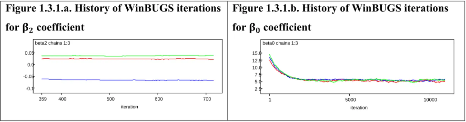
In practice, these recommendations can be implemented in two ways. One of them is checking trace plots of the sample values versus iteration to look for evidence when the simulation appears to have stabilized. Another effective method of checking convergence is running multiple chains with different starting values. For example, Figures 1.3.1.a and 1.3.1.b below illustrate iteration
process for and coefficients with three different sets of initial values that were obtained in this research. Each chain of the generated values is marked by different color. Figure 1.3.1.a exhibits estimates lacking convergence, since each chain goes in near parallel fashion and likely results in significantly different estimates for coefficient. In contrast, Figure 1.3.1.b shows an example of good convergence. Although the chains started at different initial points, they
overlapped many times, and likely result in estimates with insignificant difference.
Figure 1.3.1.a. History of WinBUGS iterations for coefficient beta2 chains 1:3 iteration 359 400 500 600 700 -0.1 -0.05 0.0 0.05
Figure 1.3.1.b. History of WinBUGS iterations for coefficient beta0 chains 1:3 iteration 1 5000 10000 2.5 5.0 7.5 10.0 12.5 15.0
To improve convergence, Gelman et al. (2004) recommended applying standardization of the covariates to have mean zero and standard deviation one, and considering better parameterization of the model to improve orthogonality of the joint posterior distribution. Since large
autocorrelation between the subsequent elements of the Markov chain can be a reason of estimates’ divergence, Neal (1995) offered using ordered over-relaxation of the parameters’ distributions to suppress the autocorrelation in the chain. This method replaces an old value,ψi, by a new value,ψi', in three steps:
1)independently generates K random values from the conditional distributionπ
(
ψi|{ψj}j≠i)
;2)arranges these K values and the old value, , in non-decreasing order:
) ( ) ( ) 1 ( ) 0 ( ... ... K i i r i i i ψ ψ ψ ψ ψ ≤ ≤ ≤ = ≤ ≤
where r is an index corresponding to the order of the old value;
3)selects a new value for a component i, (K r), where K is a parameter of this method.
i i'=ψ −
ψ
Taking into account that each step of the method requires additional computational time
of autocorrelation in the chain. He showed that even quite high autocorrelation can be effectively suppressed by setting a value of K to around 20.
1.4. Frequentist Evaluation of the Bayesian Inferences
I use objective frequentist criteria to evaluate the performance of estimators obtained by using a Bayesian approach. These frequentist properties are considered as being embedded in a sequence of repeated samples. According to Gelman et al. (2003), the Bayesian notion of stable estimation implies that for a fixed model, the posterior distribution approaches a point as more data arrive and leads in the limit to inferential certainty. Thus, if the hypothesized family of probability models contains a true distribution and assigns it a nonzero prior density, then as more information about parameter vector
ψ
arrives, the posterior distribution converges to the true value of . Specifically, I will judge an estimator in terms of its finite sample size bias and mean square error, defined by0 ψ ψˆ 0 0 ψ
[
ˆ
(
)
|
]
)]
(
ˆ
[
ψ
y
=
E
ψ
y
ψ
−
ψ
Bias
(1.4.1)where ψˆ(y) is an estimate of
ψ
0 and a function of available datay
.]
|
)
)
(
ˆ
[(
)]
(
ˆ
[
2 0 0 ψy
ψ
ψ
y
=
E
ψ
−
ψ
MSE
(1.4.2)Evaluation of a Posterior Credible Set
A set in the parameter space S Eis called a 1-α credible set for ψ, if having observed
Y = y ,
P(ψ S |y) = 1-α.
I will evaluate how well such credible sets behave as 1-α confidence sets. Specifically, I will use simulation to estimate how close the attained coverage rate of a 1-α credible set is to 1-α.
Comparing the Properties of the Estimators
I will assess and compare the frequentist properties of the Gibbs Sampler estimator to the properties of the corresponding ordinary least squares (OLS) estimator. For an estimator θˆ of a parameter θ, I will use simulation to obtain N values { }θˆi from independently generated data sets under the distribution determined by θ and let u (ˆ 2
i = θ θi− ) , i = 1, 2,…, N. Then, I will compute
1
∑
1
Approximate (1- )% confidence interval for the MSE is then given by
/
It is also reasonable to test hypothesis of equality of two competing MSE estimators based on independent random samples, the OLS MSE estimator and the Gibbs Sampler MSE estimator:
: :
with a test statistic
~ , /
w
is a size of the samples that were used in simulations to get Gibbs Sampler MSE estimate, ;
here
is a size of the samples that were used in simulations to get OLS MSE estimate, . k is a number of estimates to be estimated by Bayesian and OLS approaches to estimate the test statistic, T. In this case, there are 4 parameters to be estimated: MSE mean and variance for both Bayesian and OLS methods.
1.5. Hierarchical Bayesian Modeling
Broadly speaking, Bayesian hierarchical modeling arises in the context of (1.1.1) when the prior density π ψ( ) = π ψ η( | ) is specified conditional on unobserved parameters η that are
themselves viewed as random variables having a known density, denoted . The joint posterior distribution of parameters (
ψ η
,
) in (1.1.1) can then be expressed as
(
, |)
( | ) ( | ) ( )( ) y( ) ( | ) ( ) f p L p f π η η π ψη y = y ψ ψ ∝ ψ ψ y π η η (1.5.1) where now f( )y =∫∫
f( | ) ( | ) ( )y ψπ η ηψ p d dψ η.This approach allows greater flexibility in expressing what is known about the parameter ψ before any data are collected. This two level hierarchical model can be extended to a third level by specifying a prior density on η. This process of adding levels can be continued. Typically, a diffuse prior is used for the final level.
For example, Scollnik (2001) applied hierarchical approach to modeling the workers’ insurance relative claim frequency denoted by for a class of workers i in a year j. He assumed that the claim frequencies are conditional on latent variables {
ij
X
}
i
θ and , independent and distributed according to the following model:
Level 1: ) / 1 , ( ~ , |θi τ12 θi τ12 ij N X , i = 1, 2,…, 133, j = 1, 2,…, 7 (1.5.2)
Reasonably arguing that different workers’ insurance classes should relate to each other, Scollnik assumed that the estimates of the latent class means represent a sample from the population of all workers’ classes means, and there is no prior information to distinguish one class mean from another. Therefore, Scollnik assigned a distribution of higher level on the parameters of the claim frequency distribution: Level 2: ) / 1 , ( ~ , | 22 2 2 μ τ τ μ θi N ~ 0.001, 0.001
To model vague knowledge of the parameters of the class means’ distribution, Scollnik applied non-informative diffuse prior distributions on the precision hyperparameter, 1 σ , and on the mean of the class means distribution:
Level 3: ) 001 . 0 , 001 . 0 ( ~ ) 1000 , 0 ( ~ 2 2 Gamma N τ μ
Further, applying Gibbs Sampler method, Scollnik estimated the parameters of the hierarchical model (1.5.2) for the first six years
{
* *}
6 * 2 * 1 * * ( , ,..., ), i i i i i θ θ θ τ θ = =
ψ , i=1,…,133, and made
1.6. Studies on Global Warming
According to the free, on-line encyclopedia Wikipedia, global warming refers to the increase in the average temperature of the Earth’s near-surface air and oceans in recent decades and its projected continuation. The term global warming is an example of the broader term “climate change,” which can also refer to another term “global cooling.” Although the United Nations Framework Convention on Climates Change (2007) uses the term “climate change” for human-caused change, and “climate variability” for other changes, in my research I will focus just on change in temperature at the Earth’s surface over time, ignoring further investigation of potential reasons of these changes. Researchers investigating climate changes mostly focused on collecting reliable data, applying appropriate data transformation, and modeling time trend by using simple linear regression model. Thus, Angel (1988) applied normal linear least squares regression with a time trend to year-average temperature deviations. He estimated that over the 30-year interval, from 1958 to 1987, a global temperature increase at the Earth’s surface was 0.08 per decade and significant only at the 5% level. Over the 15-year interval, from 1973 to 1987, a global temperature increase was significant and equal 0.28 per decade.
Before using simple linear regression with a time trend, Oort and Liu (1992) smoothed the data first by applying a filter with weights 1/4, 1/2, and 1/4 to successive seasonal values, except for the beginning and the end points of the period from May 1963 to December 1989. Their estimated 95% confidence intervals for the temperature increase were between 0.07 and 0.15 per decade in the Northern Hemisphere, and between 0.22 and 0.36 per decade in the Southern Hemisphere. Jones (1994) applied simple linear regression to the surface data and found significant increase in temperature by about 0.1 per decade from 1958 to 1993.
CHAPTER 2. Application of WinBUGS Software to Hierarchical
Model Estimation
WinBUGS1.4 (hereinafter, WinBUGS) is a free and publicly available software developed by a self-organized group of researchers concerned with flexible software for
Bayesian analysis of complex statistical models using MCMC methods. This project, named the Bayesian inference Using Gibbs Sampling (BUGS) project, was launched in 1989 in the Medical Research Committee and Advisory Council (MRC) Biostatistics Unit in Cambridge, UK. A new development included also the supplementary OpenBUGS project in the University of Helsinki, Finland. Further details on the project and the software itself are available at http://www.mrc-bsu.cam.ac.uk/bugs/.
WinBUGS is a useful tool for estimating Bayesian models because of two reasons. First, WinBUGS has the ability to estimate the posterior distributions of the parameters based only on their marginal prior distributions and data model specified by a researcher. Thus, WinBUGS is an invaluable tool in many cases when the joint and marginal posterior distributions of the hierarchical Bayesian model are complex and hard to derive by hand. Second, WinBUGS accommodates numerous iterations for all parameters simultaneously within a short period of time and allows keeping track of simulations with different initial values of the parameters. This iterations monitoring accommodates checking convergence of the parameters and simplifies proving validity of the Bayesian estimates. However, WinBUGS does not attempt to verify if the posterior distribution is a proper distribution. Therefore, the posterior should be additionally checked to see if it is proper after iteration process is over.
To estimate Gibbs Sampler parameters, WinBUGS needs the following information to be supplied by a user:
a) a data model; b)a data sample;
c) parameters that should be estimated;
d)initial values of the input variables having prior distributions assigned to, which are also called stochastic nodes;
e) a number of iterations to simulate;
g)a thinning rate with which an observation is selected into a final sample, or Markov chain, from a sequence of the generated values.
There are two ways of supplying the input information into WinBUGS:
a) entering the inputs by pointing at the necessary parts of a code and clicking at the buttons with commands in a menu/dialog interface of WinBUGS;
b)scripting all commands for WinBUGS in a separate file and running the script in another software in a batch mode.
Both modes require a data model, a data sample, and initial values coded in a specific BUGS programming language and supplied into WinBUGS interface. The output information can be stored either in the interface log window or saved in a separate log file. A striking advantage of the dialog mode is an opportunity to monitor iteration process and convergence of the estimates. However, the scope of using this method in simulation study is quite limited, since each run of WinBUGS should be made manually by a researcher. In contrast, the batch mode allows running decent number of simulations by invoking WinBUGS automatically from R or other software. In this case, a number of the simulations is naturally limited by the computational capacity of a computer running the simulation code. However, controlling convergence in all simulations using the batch mode is a complex technical issue that can be resolved by an advanced programmer. One of the proxy solutions to checking convergence in simulations is to use WinBUGS in the batch mode for all simulations in combination with running the same model once in a dialog mode. This test run in the dialog mode can provide useful information about flow of the data generation process in general and can help identify some problems that can be common to all iterations run in the batch model.
2.1. Running WinBUGS in a Menu/dialog Mode
There are two options for running scripts in WinBUGS models in the menu/dialog mode. The most conventional one is saving a model and a script with the other necessary inputs in two separate files. Another option is highlighting parts of a single script file containing all necessary information and running them in the WinBUGS interface step by step. These methods have the same sequence of steps but differ slightly in coding. I describe below running WinBUGS in a menu/dialog mode from a single file on the example of my research model. In this example, I use
the first five observations of the applied data set. The exact code with full data set that I used in the research is provided in Appendix B.
An algorithm for estimation my research model in WinBUGS is as follows:
1. Open a file containing a model script by pointing to “File” option on the tool bar of WinBUGS interface and clicking the “Open” option once with left mouse button (hereinafter, LMB);
2. Make WinBUGS check that the model description fully defines a probability model in the next steps:
a) Highlight a part of the code containing description of the model, constants and variables used. The corresponding part of the code below starts with a word “model”, then describes constants and variables, and specifies the model with prior distributions on all model parameters, and ends with the final squiggle bracket in the attached code. To note, a sign # make WinBUGS skip a part of the row following this sign that can be used to provide brief
explanatory information.
# 1. Research model with conjugate priors, a linear trend and AR(1) term model const T=5; var Y[T], t; { for(t in 2:T) {
Y[t] ~ dnorm(theta.Y[t], tau.y)
theta.Y[t] <- beta0+ beta1*t + beta2*Y[t-1] }
# Prior
beta0 ~ dnorm(beta0.c, beta0.tau) #non-informative diffuse normal distn beta1 ~ dnorm(beta1.c, beta1.tau) #non-informative diffuse normal distn beta2 ~ dnorm(beta2.c, beta2.tau) #non-informative diffuse normal distn tau.y ~ dgamma(0.001,0.001)
sigma.y <-pow((1/tau.y), 0.5)
beta0.c ~ dnorm(0, 1.0E-6) #non-informative diffuse normal distn beta0.tau ~ dgamma(0.001, 0.001)
beta1.c ~ dnorm(0, 1.0E-6) #non-informative diffuse normal distn beta1.tau ~ dgamma(0.001, 0.001)
sigma.beta1<-pow((1/beta1.tau), 0.5)
beta2.c ~ dnorm(0, 1.0E-6) #non-informative diffuse normal distn beta2.tau ~ dgamma(0.001, 0.001)
sigma.beta2<-pow((1/beta2.tau), 0.5) }
b) Point to “Model” option on the tool bar and highlight the “Specification…” option. c) Check syntax of the model by clicking once with LMB on the “check model” button in the Specification Tool window. A message saying "model is syntactically correct" should appear in WinBUGS Log window.
3. Load the data by doing the next steps:
a) Highlight a part the file containing data and starting with a command word list and ending with the last bracket in the row:
# 2. Data
list(T = 5, Y = c(14.24, 14.1,13.89,13.83,13.87))
b) Click once with the LMB on the “load data” button in the Specification Tool window. A message saying "data loaded" should appear in the WinBUGS Log window.
4. Select a number of chains to be simulated by typing a corresponding number in a white box following a “num of chains” note in the Specification Tool window. It is sensible to run several chains with different initial values to check convergence of the MCMC simulations. In my case, I initiated running three chains.
5. Compile the model by clicking once with the LMB on the “Compile” button in the Specification Tool window. A message saying "model compiled" should appear in the
WinBUGS Log window. This step specifies internal data structure and specific MCMC updating algorithms to be used by WinBUGS for the particular model.
6. Provide WinBUGS with initial values for each stochastic node that are declared in the model statement. To load the initial values, you will need to
a) Highlight the code starting with the word list and ending with the last bracket of the first set of initial values:
list(beta0=0, beta1=0, beta2=0, beta0.c=0, beta1.c=0, beta2.c=0, beta0.tau=1, beta1.tau=1, beta0.tau=1, beta2.tau=1, tau.y=1)
b) Click once with the LMB on the “load inits” button in the Specification Tool window. A message saying "chain initialized but other chain(s) contain uninitialized variables" should appear in the WinBUGS Log window.
c) Repeat the steps a) and b) for the second portion of initial values:
list(beta0=0, beta1=0, beta2=0, beta0.c=0, beta1.c=0, beta2.c=0, beta0.tau=0.01, beta1.tau=0.01, beta2.tau=0.01, tau.y=0.01)
A message saying "chain initialized but other chain(s) contain uninitialized variables" should appear again in the WinBUGS Log window.
d) Repeat the steps a) and b) for the third portion of initial values:
list(beta0=0, beta1=0, beta2=0, beta0.c=0, beta1.c=0, beta2.c=0, beta0.tau=0.0001, beta1.tau=0.0001, beta2.tau=0.0001, tau.y=0.0001)
A message saying "model is initialized" should now appear in the WinBUGS Log window.
To note, that there is no need in providing a list of initial values for every parameter in a model. You can have WinBUGS to generate initial values for any stochastic parameter by clicking with the LMB on the “gen inits” button in the Specification Tool window. In this case, WinBUGS will generate initial values by forward sampling from the prior distribution for each parameter. However, it is recommended to provide your own initial values for parameters having vague prior distributions assigned to avoid wildly inappropriate values generated by WinBUGS.
7. Set monitors to store the sampled values for the selected parameters by the sequence of the following steps:
a) Click on Inference option in the WinBUGS menu first, and then point to Sample option.
b) In the opened Sample Monitor window, type the name of each parameter in the white box following a word “node”. In my model, I gave the following names to the nodes: beta0, beta1, beta2, sigma.beta0, sigma.beta1, sigma.beta2, sigma.y.
c) Set a number of the iterations to burn-in in the white box following a “beg” note and the total number of iterations in the white box following an “end” note. Since the parameter estimates of my research model were lacking convergence in near 2000 first iterations, I specified 2000 iterations to be burn-in out of 30000 in total.
d) Click “set” button you enter information at steps a) and b)
8.Now WinBUGS is set to start a simulation that can be run in the following steps: a) Select the “Update...” option from the Model menu.
b) In the opened window Update tool, type the number of updates or iterations in the white box following “updates” note, then enter a number of iteration after which you want to make a refreshment of the distribution in white box following “refresh” note, and finally type a thinning rate in the white box “thin”. In my case, I used the 30000 updates with refreshment of the iteration process after each 100 iterations, and a thinning rate of 3 iterations.
c) Click once on the “update” button. The program will start simulating values for each parameter in the model that may take a few seconds. At the same time, the box “iteration” will show how many updates have currently been completed.
d) When the number of updates in the box following “iteration” note reach the target number of iterations stated in the box near the “end” note, the iteration process will be over. At that moment, graphical and numerical summaries on iteration process for all parameters will be set for monitoring.
9. In order to check convergence and obtain posterior summaries of the model parameters, you should click Inference option in WinBUGS interface first, and then point to “Samples...” option. To see the summary of iteration process of a parameter, you will need to enter the name of this parameter in the white box following a note “node” in the Sample Monitor menu. There are the following summary options available in the menu:
a) An option “stats” describes posterior distribution by the mean, standard deviation, MC error, median, 2.5th and 97.5th percentiles.
b) An option “history” produces a plot of all parameter values in a sequence they were generated. If more than one chain run simultaneously, a history plot will show each chain in a different color. In this case, a researcher can be reasonably confident in convergence of the parameter estimator if all chains mix well.
c) An option “density” develops a graph of the density function for the estimated parameter.
d) An option “coda” provides a list of all generated values in the chain.
If all steps of the algorithm were made correctly, WinBUGS should produce an output that is similar to the iteration summary provided in Appendix C.
2.2. Working with WinBUGS in a Batch Mode
Scripting instructions in a special language and calling the WinBUGS interface from the other software allow running WinBUGS programs without pointing at the specific parts of a code and clicking your way through the commands. This feature significantly simplifies using WinBUGS by automating routine analysis and helps using WinBUGS in simulations. An opportunity of working with WinBUGS in a batch mode is now available in R, Stata, SAS, Matlab, and Excel software.
To make use of the scripting language for a specific problem, a minimum of four pieces of information are required:
1) representation of a model in WinBUGS coding language; 2) a data set of observed or simulated values;
3) initial values for each chain;
4) a script with the commands combining the model, the data, and the initial values in an iteration algorithm.
In practice, these four pieces can be provided either in one file or in several files,
depending on complexity of the model, size of the data set, and convenience to a user. Each file may be either in a native WinBUGS format (.odc) or in the text format (.txt). I show below an application of WinBUGS in a batch mode in R in a way I used it in my simulation study.
To make the WinBUGS session open in R, a special package called R2WinBUGS should be uploaded in the R version that is installed at the computer. This package provides opportunity of calling a model, summarize inferences and monitor convergence in a table and graphs, and save the simulations in arrays for easy access in R. The WinBUGS batch mode consists of the next basic steps:
1. Write an R code describing a model and prior distributions assigned to each stochastic model parameter in a separate file. A file AR1GammaModel.txt with detailed description of my research model in R is provided in Appendix E.
2. Go to R interface and prepare a script containing R commands entering the data and initial values, uploading a model file, and making WinBUGS run iterations and summary reports. In my simulation code, a piece of code with these commands is provided below, while the
complete simulation script is attached in Appendix D. # Data loading
data<-list("T","Y")
# Declaration of the model parameters to be iterated
parameters<-c("beta0", "beta1", "beta2", "sigma.y", "sigma.beta0", "sigma.beta1", "sigma.beta2")
# Loading initial values for 3 MCMC chains
inits1<-list(beta0=0, beta1=0, beta2=0, tau.y=1, beta0.tau=1, beta1.tau=1, beta2.tau=1) inits2<-list(beta0=0, beta1=0, beta2=0, tau.y=0.01, beta0.tau=0.01, beta1.tau=0.01, beta2.tau=0.01)
inits3<-list(beta0=0, beta1=0, beta2=0, tau.y=0.0001, beta0.tau=0.0001, beta1.tau=0.0001, beta2.tau=0.0001)
inits<-list(inits1, inits2, inits3)
# Invoking an auxiliary sub package “arm” of the R2WinBUGS package library("arm")
# Applying bugs function entering inputs and running WinBUGS from R AR1bugs.sim<- bugs(data, inits, parameters,
“D:/KSU_Research/Final/AR1GammaModel.txt", n.chains=3, n.iter=5000, bugs.directory="c:/Program Files/WinBUGS14/",
working.directory="D:/KSU_Research/Final/Results/", clearWD=FALSE, debug=FALSE) # Storing BUGS simulation results in the R interface operation memory
attach.bugs(AR1bugs.sim)
In the code above, bugs function plays a key role in running WinBUGS from R interface. This function takes data, initial values and assigns parameters of iteration process as inputs,
automatically writes a WinBUGS script, calls the model, and saves the simulations results. In order to make this function run, a set of the function parameters should be defined:
data is a named list of variables having data and used in the WinBUGS model. In the code above, the data inputs are the data lists named Y and T that were earlier assigned a data set and a number of observations in this data set respectively.
inits is a R set of initial values for each iteration chain. Before, I assigned 3 sets called inits1, inits2, and inits3 that include initial values for all model stochastic parameters for each of three chains iterated further by WinBUGS. A number of the Markov chains should corresponds to the bugs function argument n.chain declaring a number of chains to be generated by
WinBUGS. In this, case n.chain is assigned a value 3. Alternatively, if inits=NULL, initial values are generated by WinBUGS.
parameters is a character vector of the names of the stochastic parameters which
WinBUGS should take records on. In my code, these parameters are beta0, beta1, beta2, sigma.y, sigma.beta0, sigma.beta1, and sigma.beta2.
The fourth argument of the bugs function must be a note containing a path and a file name that contains description of the model in WinBUGS code. The extension of the model file can be either “.bug” or “.txt”. In my code, a note specifying a file with the model description is D:/KSU_Research/Final/AR1GammaModel.txt
n.iter is a number of total iterations per chain including a number of burn-in iterations that is 5000 iterations in my code.
bugs.directory is a directory that contains the WinBUGS executable files that were stored at c:/Program Files/WinBUGS14/.
working.directory sets a directory storing the WinBUGS' input and output files during execution of this function that in my case was D:/KSU_Research/Final/Results/.
clearWD is a logical argument indicating whether the WinBUGS’ input and output files should be removed from the operation memory after WinBUGS has finished. A logical value FALSE assigned to argument clearWD in my code orders WinBUGS save all output in separate files in working directory assigned above.
debug is a logical argument with a default FALSE value making WinBUGS close automatically when the script has finished running, otherwise WinBUGS remains open for further investigation.
Further bugs arguments takes default values, if a user does not assign any specific values to them. In my simulation code, the following arguments are assigned default values:
n.burnin is a number of iterations in a sample of generated values to be burnt in at the beginning. The default for burn-in values is discarding the first half of the simulations, n.iter/2, that in my case is 2500 iterations.
n.thin is a thinning rate and must be a positive integer. The default is maximum value selected between 1 and rounded down to a value calculated using a formula: (n.chains * (n.iter-n.burnin) / 1000)). The default thin rate will be assigned if there are at least 2000 simulations. In my case, a thinning rate is 5.
bin is a number of iterations between saving of results. Default value used in my code is to save only at the end of the iteration process.
DIC is a logical argument with a default TRUE value computing deviance, pD, and DIC. digits is a number of significant digits used for WinBUGS input.
codaPkg is a logical argument with a default FALSE value that arrange a bugs output object to be returned. If the TRUE value assigned, the file names of WinBUGS output are returned for easy access by the coda package through function read.bugs.
bugs.seed is a random seed for WinBUGS with a default no seed value.
summary.only with a default TRUE value limits the WinBUGS output to a short parameter summary for a quick analyses. In my case, temporary created files are not removed.
save.history with a default TRUE value generate trace plots for the declared parameters of interest.
3. When a part of the code stated above runs, a WinBUGS window will appear and R interface will freeze up. At this time the model will now run in WinBUGS. Running a model might take awhile, depending on the number of iterations and complexity of the model. You will be able to see details of the iterations exhibited in the log window within WinBUGS. When WinBUGS finishes iterations, its window will close and R will work again.
4. If an error message appears at the log window, it is recommended to re-run the model in R with debug option set in “TRUE” value. After this change in debug settings, the batch mode will provide all WinBUGS output summary and graphs to the screen. Examining the tables and graphs can help identifying potential problem in coding.
Chapter 3. Research Results
3.1. Autoregressive Research Model
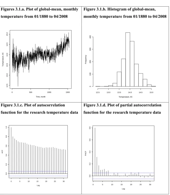
Although, in common usage, the term “global warming” is often referred to human influence on the global climate, my research is focused on change in temperature at the Earth’s surface over time without digression into further investigation of potential causes of these changes. Santer et al. (1996) argued that the thermal structure of the atmosphere is not the same in the Northern and Southern hemispheres primarily due to an asymmetry in observed ozone changes. Therefore, stratospheric cooling in the Northern Hemisphere could be different from cooling in the Southern Hemisphere. However, in order to simplify the exposition here, I ignored these potential differences and combined the data from both hemispheres. I used global-mean monthly, annually, and seasonally adjusted temperature at the Earth’s surface in 0.01 degrees Centigrade (˚C) from January 1880 to April 2008 that were provided by NASA’s Goddard Institute for Space Studies1. Since NASA’s data were in 0.01 and relative to the base period temperature of 14 , I transformed the original data by multiplying the official data by 100 and adding 14 to obtain an absolute monthly global-mean temperature in degrees Centigrade. These data are presented below in Figures 3.1.a – 3.1.d. In modeling monthly temperature data, I took into consideration autocorrelation function and partial autocorrelation function estimated for the available data. The autocorrelation function of order k, or ACF(k), gives the gross correlation, or
, betw e te n he temperature at time t, , and the temperature at lag k, :
,
(3.1.1) A theoretical autocorrelation function is estimated in a sample by what is called a correlogram, given by:
∑
∑ (3.1.2)
A partial autocorrelation function of order k, or PACF(k), is a correlation between and net of intervening effects of the lagged temperatures observed between these two observations:
1 The data used in this research are extracted from the official web-site of GISS NASA:
|
where | , … , is the minimum mean-squared error predictor of by
, … , . In practice, PACF(k) is estimated using a linear predictor of
| , … , , (3.1.3) , … , : .4) , (3.1 where , , … , = , , … , , , , … , .
In the NASA’s monthly temperature data set, the estimated ACF on Figure 3.1.c is decaying slowly with the highest correlation observed between the current observation and its first lag, around 0.8. A graph of the estimated PACF at Figure 3.1.d exhibits the first nine PACF coefficients irregularly declining from near 0.8 to 0.1, marginally significant coefficient at lag 12, and two significant PACF coefficients at lag 20 and lag 24. This oscillating pattern of PACF with near a dozen of significant partial correlation coefficients and slow decay in ACF are evidence of potential non-stationarity and significant time trend in the monthly temperature data. Although the true data generating process likely have an intricate autoregressive structure, I chose a linear model with a time trend and the first order autoregressive term denoted by AR(1) because in numerous empirical studies the first order autoregression is proved to be a reasonable model even for very complex underlying processes (Greene (2003)). Therefore, my research model is the first reliable pass to the next comparative analysis of OLS and hierarchical Bayesian estimates, while further refinement of the model by applying autoregressive terms of higher order is left f the futureor work in the field. Let
(3.1.5)
| , , ,
, , , ~ ,
|
where is a white noise time-series process where each element of the sequence is jointly independent and normally distributed: ~ 0, , ∞ ∞;
β1 represents a linear trend in the means as time, denoted by t, increases.
Figures 3.1.a. Plot of global-mean, monthly temperature from 01/1880 to 04/2008
Figure 3.1.b. Histogram of global-mean, monthly temperature from 01/1880 to 04/2008
Figure 3.1.c. Plot of autocorrelation
function for the research temperature data
Figure 3.1.d. Plot of partial autocorrelation function for the research temperature data
Time, month Tem per at ur e, 0C 0 500 1000 1500 1 2. 5 13 .0 13. 5 1 4. 0 14. 5 1 5. 0 Temperature, 0C F req uency 12.5 13.0 13.5 14.0 14.5 15.0 0 100 200 300 400 0 5 10 15 20 25 30 0 .0 0 .2 0 .4 0 .6 0 .8 1 .0 Lag AC F 0 5 10 15 20 25 30 0. 0 0 .2 0. 4 0 .6 0. 8 Lag PA CF
Hierarchical Bayesian Model for Testing Existence of the Global Warming Level 1: | , , , , ~ , (3.1.6.) Level 2: 1 ~ 0.001, 0.001 | , ~ , | , ~ , | , ~ , Level 3: ~ 0, 10 1 ~ 0.001, 0.001 ~ 0, 10 1 ~ 0.001, 0.001 ~ 0, 10 1 ~
where , denotes a gamma distribution with a shape parameter and a scale parameter 1/ .
0.001, 0.001
WinBUGS specification of a normal distribution requires two parameters: mean and precision parameter, 1 σ . A gamma distribution of the precision parameter, , implies an inverse scaled χ distribution of the variance, . The precise form of the diffuse priors is believed to be not very important in this case. Since the collected data comprise rather large sample, 1539 observations, the data likelihood should overwhelmingly dominate in forming posterior distribution. In the model (3.1.2), parameters of interest are as follows:
) , , , , , , , , , ( 2 2 2 2 2 1 0
β
β
μ
0μ
1μ
2σ
0σ
1σ
2σ
Yβ
β β β β β β = ΨThe joint posterior distribution for the par meters of interest follows equation (3.1.3):
, , , , , , , , ,
, , , ∏ | , , , (3.1.3)
a
A marginal posterior distribution for each parameter of interest can be found in theory by integrating joint posterior distribution over the other parameters. However, there are problems here in deriving an exact form for a joint posterior distribution in equation (3.1.3) and a marginal posterior distribution for each parameter because of the complex form of the model. In this case, WinBUGS will estimate these distributions by using approximations.
3.2. Estimation Results for the Research Models
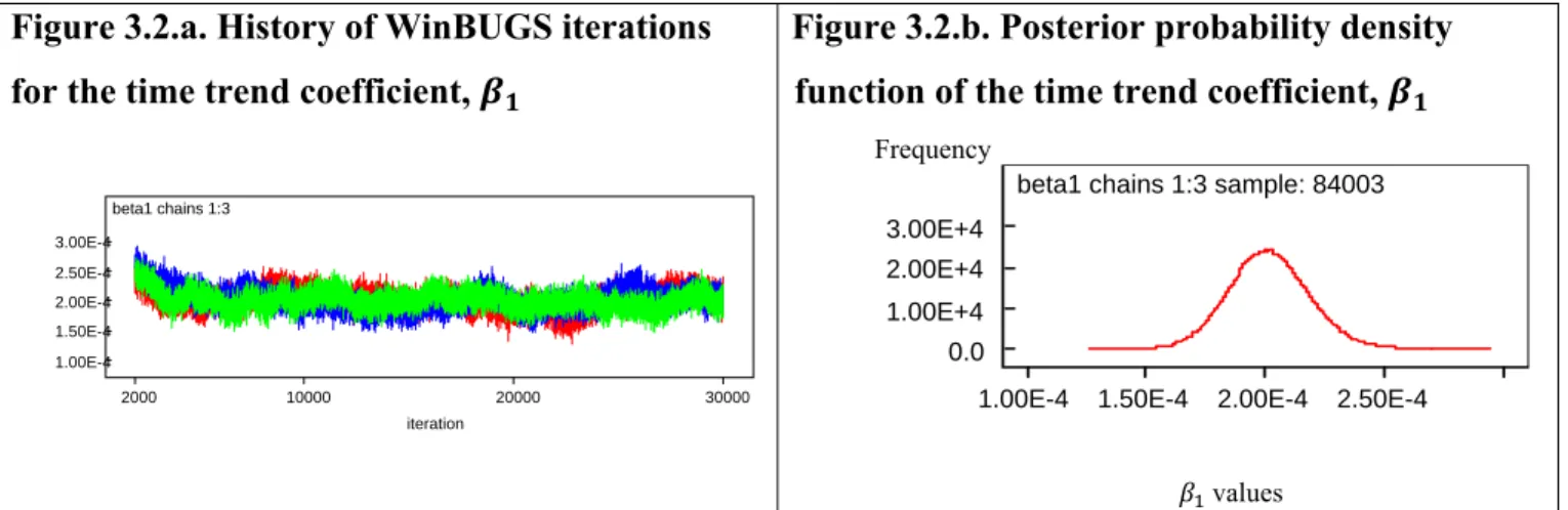
Initial trial runs of the model in WinBUGS showed that it took near 2000 iterations of the model parameters’ estimates to converge. Therefore, I assigned 2000 iterations out of 30000 in total to be burnt in. The final estimation results presented below are based on the WinBUGS output excluding burn-in iterations and having a thinning rate of 3 iterations. The iteration history for all Gibbs Sampler estimates suggests about quite good mixing of the iterations in the chains and convergence of the estimates. Estimation summary of the hierarchical Bayesian model and plots of the distribution formation are provided below, while detailed WinBUGS output summary on all model parameters is provided in Appendix C.
Figure 3.2.a. History of WinBUGS iterations for the time trend coefficient,
beta1 chains 1:3 iteration 2000 10000 20000 30000 1.00E-4 1.50E-4 2.00E-4 2.50E-4 3.00E-4
Figure 3.2.b. Posterior probability density function of the time trend coefficient,
Frequency
beta1 chains 1:3 sample: 84003
1.00E-4 1.50E-4 2.00E-4 2.50E-4 0.0 1.00E+4 2.00E+4 3.00E+4 values | , , , ~ , | 5.383 0.000202 0.6047 , MC error (0.0167) (0.00006) (0.00123)
0.184
The estimated 95% credibility interval for the time trend coefficient is (0.000169, 0.000237). Since a plot of the posterior distribution of the time trend coefficient on Figure 3.2.b. shows that 100% of the distribution of estimates is above 0 values, there is strong evidence of global warming. The 95% credibility interval for also suggest that there is 95% chance that the global temperature increase is between 0.000169 and 0.000237 per month, or between 0.0203 and 0.0284 per decade.
OLS Estimation of Global-mean Monthly Temperature
A brief summary of the estimation results for the OLS model is given below, while detailed WinBUGS output summary is attached in Appendix C. Now letting , 0, 1, 2
denote ordinary least squares estimators:
| 5.283 0.0002 0.612
.6805 SE (0.274) (0.000015) (0.020)
0
MSE 0.182
The approximate 95% confidence interval for the time trend coefficient includes values from 0.000103 to 0.000339.
Testing hypothesis for existence of the global warming, we obtain:
: 0
: 0
0
13.59 ~
p-value = Prob(| | 13.59) <2 10
Since the p-value of the time trend coefficient, , is less than 1%, there is strong evidence of the global warming. At 95% confidence, the global temperature tends to grow from
0.000103 to 0.000339 per month or 0.0124-0.0406 per decade. Since 95% credibility interval and 95% confidence interval overlap, there is no evidence of significant difference in the Gibbs Sampler estimate and OLS estimate.
Chapter 4. Simulation study comparing OLS estimators and
Hierarchical Bayes estimators
4.1. Parameter Specification
In the simulation study, I generated samples of 10, 30, 100, and 1000 observations from the model (3.1.1) with the regression parameters fixed at the specific values:
0, 1, 0.5, 1.
Given different sample sizes and data generated from the model (3.1.1), the Bayesian and OLS estimators were obtained, and their performance was evaluated in terms of bias and mean square error. The Bayesian simulations were run for three chains starting with the following initial values:
1)The first s t of the initial values, hereinafter initialse 1:
0, 0, 0, 1, 1, 1.
2)The second set of the initial values, hereinafter initials 2:
0, 0, 0, 100, 100, 100.
3)T eh third set of the initial values, initials 3:
0, 0, 0, 1000, 1000, 1000.
Since starting values for were not assigned, they were randomly selected by
WinBUGS from the model prior distribution such that the precision parameter, , following the Gamma distribution:
1
~ 0.001, 0.001
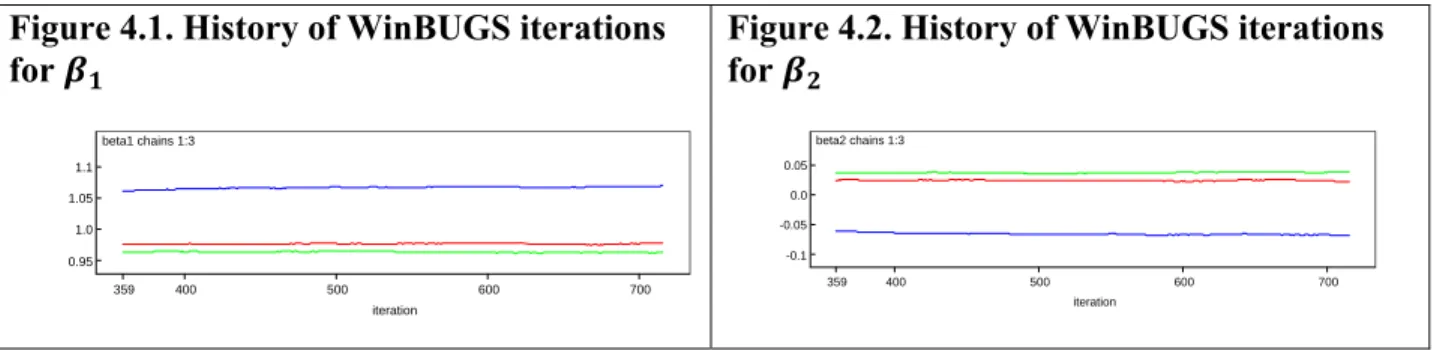
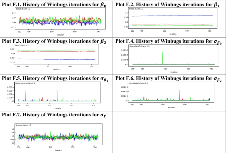
Tables 4.1, 4.2, 4.3 and 4.4 below summarize estimation results from 100 simulations of the samples with 10, 30, 100, and 1000 data points. The history of iteration process for and
coefficients in the test run of the research model with a generated sample of 1000 data points is exhibited on Figure 4.1 and Figure 4.2 below, while more detailed WinBUGS output summary for the test run is provided in Appendix F. The graphs below suggest that the estimates obtained in the test run do not converge and depend on the initial values, since all three lines representing three different chains for and coefficients are almost parallel.
Figure 4.1. History of WinBUGS iterations for beta1 chains 1:3 iteration 359 400 500 600 700 0.95 1.0 1.05 1.1
Figure 4.2. History of WinBUGS iterations for beta2 chains 1:3 iteration 359 400 500 600 700 -0.1 -0.05 0.0 0.05
Problems with the estimates’ convergence in the test run of the model suggest potential issues with the estimates’ divergence in all runs of the research model. Therefore, further research in the field can focus on improving convergence by considering the following options:
a) Developing a better parameterization of the model to improve orthogonality of the joint posterior distribution.
b)Standardization of the covariates to have mean zero and standard deviation one. c) Using ordered over-relaxation of the parameters distributions to suppress random walk autocorrelation between two subsequent elements in a Markov chain. According to Neal (1995), this method generates a K number of candidates for a subsequent element of the chain, ranks the previous element and the candidates for the next element in non-decreasing order, and selects the next element with a rank that equals the difference between the maximum rank in the overall list and the rank of the previous element of the chain.
4.2. Comparison of OLS Estimators and Hierarchical Bayes Estimators
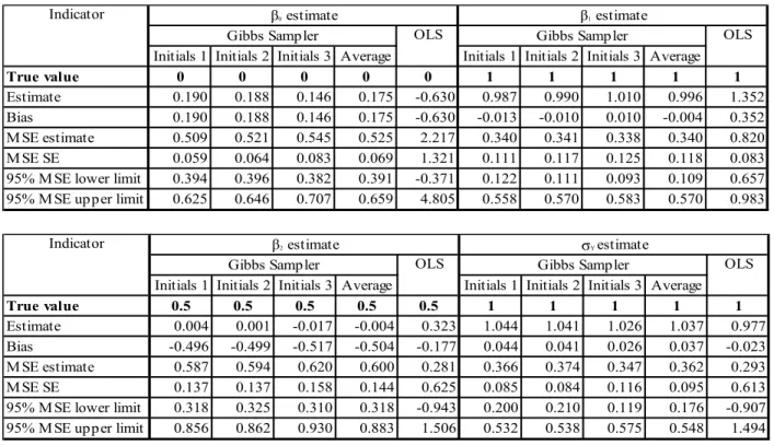
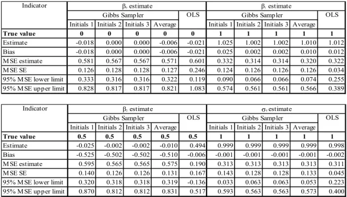
Results of the simulation study for the sample sizes of 10, 30, 100, and 1,000observations are summarized below in Tables 4.1, 4.2, 4.3, and 4.4 respectively. The estimated biases of the Gibbs Sampler estimator of and tend to be lower in absolute values than the biases of the corresponding OLS estimators for all sample sizes. The estimated MSE of the Gibbs Sampler estimators of and are lower in average than the MSE of the OLS estimators in all sample sizes. In contrast, the biases of Gibbs Sampler estimators and are higher in absolute values than the corresponding OLS estimators. The estimated MSE of the Gibbs Sampler for and estimators are in average higher than the MSE of the OLS estimators. However, the formal tests detected significant difference in MSE only for estimators for the
small samples of size 10 and 30 observations. The other differences in MSE are statistically insignificant. All details on testing significance of difference in MSE are given in Appendix G.
To recap, my simulation study showed that the Gibbs Sampler estimator for a time trend coefficient tends to be less biased than the OLS estimator in samples of all sizes, while the Gibbs Sampler estimator is more precise for a time trend only in small samples of 10 and 30 observations. In the bigger samples, Gibbs Sampler and OLS estimators are similar in their precision.
Table 4.1. Estimation results from 100 simulations with a sample size 10 data points
Initials 1 Initials 2 Initials 3 Average Initials 1 Initials 2 Initials 3 Average True value 0 0 0 0 0 1 1 1 1 1 Estimate 0.435 0.424 0.560 0.473 -1.019 0.933 0.934 0.990 0.952 1.633 Bias 0.435 0.424 0.560 0.473 -1.019 -0.067 -0.066 -0.010 -0.048 0.633 M SE estimate 0.611 0.550 0.680 0.614 4.030 0.365 0.299 0.388 0.351 1.520 M SE SE 0.098 0.053 0.120 0.090 2.447 0.150 0.199 0.171 0.173 0.076 95% M SE lower limit 0.419 0.446 0.440 0.435 -0.766 0.072 -0.090 0.053 0.012 1.371 95% M SE upper limit 0.804 0.653 0.920 0.792 8.825 0.658 0.689 0.723 0.690 1.668
Indicator β0 estimate β1 estimate
Gibbs Sampler OLS Gibbs Sampler OLS
Initials 1 Initials 2 Initials 3 Average Initials 1 Initials 2 Initials 3 Average True value 0.5 0.5 0.5 0.5 0.5 1 1 1 1 1 Estimate 0.020 0.011 -0.077 -0.015 0.168 1.071 1.130 1.097 1.099 0.906 Bias -0.480 -0.489 -0.577 -0.515 -0.332 0.071 0.130 0.097 0.099 -0.094 M SE estimate 0.605 0.664 0.732 0.667 0.494 0.474 0.475 0.433 0.461 0.337 M SE SE 0.092 0.168 0.175 0.145 1.107 0.040 0.022 0.126 0.063 1.265 95% M SE lower limit 0.425 0.335 0.389 0.383 -1.674 0.395 0.431 0.186 0.337 -2.141 95% M SE upper limit 0.784 0.993 1.074 0.950 2.663 0.553 0.519 0.680 0.584 2.816
Indicator β2 estimate σY estimate
Gibbs Sampler OLS Gibbs Sampler OLS
Table 4.2. Estimation results from 100 simulations with a sample size 30 data points
Initials 1 Initials 2 Initials 3 Average Initials 1 Initials 2 Initials 3 Average True value 0 0 0 0 0 1 1 1 1 1 Estimate 0.190 0.188 0.146 0.175 -0.630 0.987 0.990 1.010 0.996 1.352 Bias 0.190 0.188 0.146 0.175 -0.630 -0.013 -0.010 0.010 -0.004 0.352 M SE estimate 0.509 0.521 0.545 0.525 2.217 0.340 0.341 0.338 0.340 0.820 M SE SE 0.059 0.064 0.083 0.069 1.321 0.111 0.117 0.125 0.118 0.083 95% M SE lower limit 0.394 0.396 0.382 0.391 -0.371 0.122 0.111 0.093 0.109 0.657 95% M SE upper limit 0.625 0.646 0.707 0.659 4.805 0.558 0.570 0.583 0.570 0.983
Indicator β0 estimate β1 estimate
Gibbs Sampler OLS Gibbs Sampler OLS
Initials 1 Initials 2 Initials 3 Average Initials 1 Initials 2 Initials 3 Average True value 0.5 0.5 0.5 0.5 0.5 1 1 1 1 1 Estimate 0.004 0.001 -0.017 -0.004 0.323 1.044 1.041 1.026 1.037 0.977 Bias -0.496 -0.499 -0.517 -0.504 -0.177 0.044 0.041 0.026 0.037 -0.023 M SE estimate 0.587 0.594 0.620 0.600 0.281 0.366 0.374 0.347 0.362 0.293 M SE SE 0.137 0.137 0.158 0.144 0.625 0.085 0.084 0.116 0.095 0.613 95% M SE lower limit 0.318 0.325 0.310 0.318 -0.943 0.200 0.210 0.119 0.176 -0.907 95% M SE upper limit 0.856 0.862 0.930 0.883 1.506 0.532 0.538 0.575 0.548 1.494
Indicator β2 estimate σY estimate
Table 4.3. Estimation results from 100 simulations with a sample size 100 data points
Initials 1 Initials 2 Initials 3 Average Initials 1 Initials 2 Initials 3 Average True value 0 0 0 0 0 1 1 1 1 1 Estimate -0.018 0.000 0.000 -0.006 -0.021 1.025 1.002 1.002 1.010 1.012 Bias -0.018 0.000 0.000 -0.006 -0.021 0.025 0.002 0.002 0.010 0.012 M SE estimate 0.581 0.567 0.567 0.571 0.601 0.332 0.314 0.314 0.320 0.322 M SE SE 0.126 0.128 0.128 0.127 0.246 0.124 0.126 0.126 0.126 0.034 95% M SE lower limit 0.333 0.316 0.316 0.322 0.119 0.090 0.066 0.066 0.074 0.255 95% M SE upper limit 0.828 0.817 0.817 0.821 1.083 0.574 0.561 0.561 0.566 0.389
Indicator β0 estimate β1 estimate
Gibbs Sampler OLS Gibbs Sampler OLS
Initials 1 Initials 2 Initials 3 Average Initials 1 Initials 2 Initials 3 Average True value 0.5 0.5 0.5 0.5 0.5 1 1 1 1 1 Estimate -0.025 -0.002 -0.002 -0.010 0.494 0.999 0.999 0.999 0.999 0.998 Bias -0.525 -0.502 -0.502 -0.510 -0.006 -0.001 -0.001 -0.001 -0.001 -0.002 M SE estimate 0.595 0.565 0.565 0.575 0.190 0.313 0.313 0.313 0.313 0.311 M SE SE 0.140 0.126 0.126 0.131 0.167 0.143 0.128 0.128 0.133 0.045 95% M SE lower limit 0.320 0.318 0.318 0.319 -0.136 0.033 0.063 0.063 0.053 0.223 95% M SE upper limit 0.870 0.812 0.812 0.831 0.517 0.593 0.563 0.563 0.573 0.400
Indicator β2 estimate σY estimate
Gibbs Sampler OLS Gibbs Sampler OLS
Table 4.4. Estimation results from 100 simulations with a sample size 1000 data points
Initials 1 Initials 2 Initials 3 Average Initials 1 Initials 2 Initials 3 Average True value 0 0 0 0 0 1 1 1 1 1 Estimate -0.018 0.000 0.000 -0.006 -0.021 1.025 1.002 1.002 1.010 1.012 Bias -0.018 0.000 0.000 -0.006 -0.021 0.025 0.002 0.002 0.010 0.012 M SE estimate 0.581 0.567 0.567 0.571 0.601 0.332 0.314 0.314 0.320 0.322 M SE SE 0.126 0.128 0.128 0.127 0.246 0.124 0.126 0.126 0.126 0.034 95% M SE lower limit 0.333 0.316 0.316 0.322 0.119 0.090 0.066 0.066 0.074 0.255 95% M SE upper limit 0.828 0.817 0.817 0.821 1.083 0.574 0.561 0.561 0.566 0.389
Indicator β0 estimate β1 estimate
Gibbs Sampler OLS Gibbs Sampler OLS
Initials 1 Initials 2 Initials 3 Average Initials 1 Initials 2 Initials 3 Average True value 0.5 0.5 0.5 0.5 0.5 1 1 1 1 1 Estimate -0.025 -0.002 -0.002 -0.010 0.494 0.999 0.999 0.999 0.999 0.998 Bias -0.525 -0.502 -0.502 -0.510 -0.006 -0.001 -0.001 -0.001 -0.001 -0.002 M SE estimate 0.595 0.565 0.565 0.575 0.190 0.313 0.313 0.313 0.313 0.311 M SE SE 0.140 0.126 0.126 0.131 0.167 0.143 0.128 0.128 0.133 0.045 95% M SE lower limit 0.320 0.318 0.318 0.319 -0.136 0.033 0.063 0.063 0.053 0.223 95% M SE upper limit 0.870 0.812 0.812 0.831 0.517 0.593 0.563 0.563 0.573 0.400
Indicator β2 estimate σY estimate
Chapter 5. Conclusions
I created a model including a time trend and a first order autoregressive term, and applied it to testing for the existence of the global warming. My hierarchical Bayesian research model with diffuse conjugate prior distributions took into account natural high autocorrelation between a monthly temperature observation and its first lag by incorporating an AR(1) term and placing a prior distribution on it. The parameters of the model were estimated by applying OLS and Gibbs Sampler with 30,000 iterations and three chains with the different starting values. The Gibbs Sampler estimate for the global temperature increase was between 0.0203 and 0.0284 per decade with 95% credibility. The OLS estimate for the temperature increase was between 0.0124 and 0.0406 per decade at 95% confidence, while the difference between Gibbs Sampler estimate and OLS estimate was insignificant. Moreover, since all percentiles of the posterior distribution of the Gibbs Sampler estimate for a time trend were above 0, there is strong evidence of global warming.
Second, in my simulation study I randomly generated 100 samples of 10, 30, 100, and 1000 observations from a normal distribution with a mean having a linear time trend and an AR(1) term, and the model parameters fixed at the following values: = 0, = 1, = 0.5,
= 1. Further, these parameters were estimated by OLS and by Gibbs Sampler. The Gibbs Sampler estimators with three different initial values failed to converge and were considered separately. In 100 simulations, the Gibbs Sampler estimators for an intercept and for the time trend were less biased than corresponding OLS estimators, while the reverse was true for the autoregressive parameter and error standard deviation. The difference in precision of the
estimators found by two approaches was insignificant except for the estimator of the time trend. The Gibbs Sampler estimators for MSE of the time trend coefficient were significantly smaller than the OLS estimators of MSE only in the small samples of 10 and 30 observations.
Third, although the test run in simulation study detected lack of convergence in the Gibbs Sampler estimates for the time trend and AR(1) term coefficients, my research based on the real temperature data did not show significant issues with convergence. The difference in estimates’ convergence can occur for several reasons. The distribution of the real data can differ
significantly from the assumed distribution with the mean following AR(1) model with a time trend. Therefore, the same mix of the prior distributions and the research model can result in
different convergence outcomes in the simulation study and a study based on the real data. On the other hand, a problem with convergence can be related to the parameters of the iterations process, like