Columbia River plume patterns in summer 2004 as revealed by a
hindcast coastal ocean circulation model
Yonggang Liu,1 Parker MacCready,1 and Barbara M. Hickey1
Received 23 October 2008; revised 14 November 2008; accepted 21 November 2008; published 16 January 2009. [1] Model hindcasts of the Columbia River (CR) plume
and coastal ocean circulation in summer 2004 are used to describe the subtidal evolution of plume patterns in response to local wind and to examine the plume influence on shelf circulation. It is found that a bi-directional plume occurs frequently on the Washington/Oregon shelf, during weak upwelling favorable wind events, during weakening of moderate upwelling favorable wind events, and during weak downwelling events. The high frequency of occurrence of the north plume branch indicates that the CR water will have a significant influence on the Washington shelf in summer. Citation: Liu, Y., P. MacCready, and B. M. Hickey (2009), Columbia River plume patterns in summer 2004 as revealed by a hindcast coastal ocean circulation model,Geophys. Res. Lett.,36, L02601, doi:10.1029/2008GL036447.
1. Introduction
[2] One of the basic questions of the RISE (River Influence on Shelf Ecosystem) project is why the Wash-ington (WA) shelf is more productive than the Oregon (OR) shelf [e.g., Hickey and Banas, 2003; Ware and Thomson, 2005; Thomas and Brickley, 2006]. Among many other factors, such as shelf width and bottom topography, the Columbia River (CR) is thought to play an important role. The CR plume alters stratification, nutrient pathways and circulation patterns on the shelf, and affects the marine ecosystem along the northwest Pacific coast [e.g., Hickey and Banas, 2003;Banas et al., 2009].
[3] Previous studies of the CR plume mainly relied onin situ observations [e.g., Hickey et al., 1998, 2005, 2009], which are limited in both space and time. Thus, it is difficult to obtain a complete picture of the CR plume variation on synoptic time scales, especially to resolve the highly variable plume front. Satellite remote sensing is useful in monitoring the surface fields in a larger scope, and has many applications in coastal oceanography [e.g., Thomas and Weatherbee, 2006]. However, it may not be an effective tool for monitoring the CR plume synoptic variability. Conventional satellite altimetry does not work well near the coast. Satellite-derived ocean color may work well near the coast, but frequent cloud cover is a problem for this area even in summer. Clouds may not be a problem for some infrared SST products [e.g.,Quartly and Srokosz, 2002], but the CR plume is not clearly featured in summer SST. In fact, most previous satellite studies in this area were not focused on synoptic time scales but on seasonal time scales and longer
[e.g.,Legaard and Thomas, 2006;Venegas et al., 2008]. In contrast, numerical models may provide a continuous and more complete picture of the CR plume synoptic variation. [4] The first 3D numerical modeling effort for the CR plume was Garcı´a Berdeal et al. [2002], in which the response of the CR plume to idealized mean and fluctuating winds, ambient flow, and outflow conditions was studied, and the bi-directional nature of the plume was illustrated. Recently, 3D models on unstructured grids, ELCIRC and SELFE, were developed for the CR estuary-plume-shelf system [e.g., Baptista et al., 2005; Zhang and Baptista, 2008], and realistic forcing was used; however, analysis of the modeled CR plume variability was focused on seasonal and inter-annual time scales (A. Baptista, Seasonal and inter-annual variability of the Columbia River plume: A perspective enabled by multi-year simulation databases, submitted to Journal of Geophysical Research, 2008). Another model, ROMS, was used in the RISE project to simulate the CR estuary-plume-shelf system with realistic forcing [MacCready et al., 2009]. This model uses a stretched, spherical grid (45 – 48°N, 125.5 – 121°W) with 400 m horizontal resolution in the estuary and plume region, telescoping to 9 km in the far corners, and has 20 sigma layers in the vertical direction. It is initialized and one-way nested within NCOM-CCS [Shulman et al., 2004]. Model forcing includes daily river flow from the USGS gauging station at Beaver Army Station, tides (10 constituents from the TPXO6.0 [Egbert and Erofeeva, 2002]), hourly winds, surface pressure, air temperature, humidity, and radiation (from the Northwest Modeling Consortium MM5 regional model [Mass et al., 2003]). The overall model skill was evaluated as moderate using an extensive set of observa-tions [Liu et al., 2009]. In particular, the model successfully simulated surface current subtidal variability in the near-field plume, with high correlation (0.86, significant at the 95% level of confidence) and regression (0.95) coefficients between the modeled and HF radar observed first mode principal component time series. As a follow-on study to MacCready et al.[2009] andLiu et al., [2009], this paper analyzes the model surface velocity, salinity (S) and tem-perature (T) in summer 2004 with a focus on deriving characteristic patterns of the CR plume on synoptic time scales and their impact on shelf circulation.
2. Temporal Mean Patterns and Standard Deviations of the Surface Fields
[5] The model hindcast extends from June 3 to August 31, 2004; the first several days of model spin-up are excluded and the period 06/15 – 08/31 is chosen for this analysis. The temporal mean surface S map shows a bi-directional plume near the CR mouth: the low S water Here
for
Full Article
1
School of Oceanography, University of Washington, Seattle, Wa-shington, USA.
Copyright 2009 by the American Geophysical Union. 0094-8276/09/2008GL036447$05.00
from the CR has two branches, the major one extends southwest offshore, and the minor one turns north and hugs the WA coast (Figure 1a). Temporal mean surface currents are southward over the major part of the shelf, consistent with mean upwelling favorable winds (Figure 1b). Within the northern plume branch, the mean flow is weak but directed northward. The CR plume pattern is not as clearly seen in the surfaceTas in the surfaceS; However, capping of the coastal upwelling by the plume [Hickey et al., 2005] is evident: from the CR to Grays Harbor on the WA coast, the mean Tis higher than along the other part of the coast (Figure 1b).
[6] The time series of the surface fields have been 36 hr low-pass filtered to focus on subtidal variability. For surface S and T, subtidal variability is quantified by standard deviation. For velocity time series, the variability is shown as ellipses of the principal axis currents. Subtidal variability of the surfaceSis generally larger in the mean plume area than in the rest of the shelf area, with maximum variability near the CR mouth (Figure 1c). This demonstrates the modification of surface water properties by the plume. As with S, subtidal variability of surface velocity is also generally larger in the mean plume area (Figure 1e). The principal axis currents are as great as 0.4 – 0.5 m s 1north of the CR mouth on the WA coast, a result of the variability of the CR plume northern branch. SurfaceThas larger subtidal variability near the coast than offshore due to the variation
of the coastal upwelling. The variability is smaller along the coast that is most affected by the plume (from south of the CR on the OR coast to Grays Harbor on the WA coast), indicating the capping effect (Figure 1d).
3. Typical Patterns of Subtidal Surface Fields
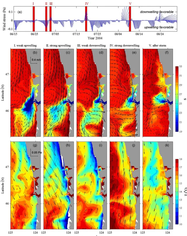
[7] To illustrate subtidal variation of surface fields in response to different wind forcing, daily mean surface fields are examined for five typical cases: weak upwelling favor-able winds, moderate to strong upwelling favorfavor-able winds, weak downwelling favorable winds, strong downwelling favorable winds, and a day after the passage of a summer wind storm, on 06/24, 06/30, 07/02, 07/19 and 08/09, respectively (Figure 2a).
[8] After three consecutive days of weak upwelling favorable winds (daily averaged wind stress, ts, of 0.03 – 0.04 Pa), the CR plume was bi-directional on 06/24/2004 (Figure 2b), similar to the summer mean pattern. The patterns of surfaceS,Tand velocity show that most fresh/ warm river water first turns right (Figure 2g) as the northern plume branch along the WA coast, and then the fresh water on the offshore edge of the plume is brought southward by the weak southward flow. While mixing with the ambient colder and saltier water, it is spread southwestward off the OR outer shelf and slope. Thus, the low S water in the northern plume branch is ‘‘new’’, and that in the southern
Figure 1. (a) Temporal mean surface salinity superimposed with currents, (b) temperature superimposed with wind stress,
(c) standard deviation (std) of salinity, (d) std of temperature, and (e) principal axis surface currents from the model output, averaged during June 15 – August 31, 2004. The std values are calculated using 36 hr low-pass filtered time series. The isobaths of 50, 100, 200 and 1000 m are also shown on the maps. Abbreviations: Washington (WA), Oregon (OR), Grays Harbor (GH), Willapa Bay (WB), and Columbia River (CR).
Figure 2. (a) 36-hr low-pass filtered time series of wind stress spatially averaged over the plume area (124.8 – 123.8°W, 45.8 – 46.8°N). (b – f) Daily mean surface salinity superimposed on surface currents and (g – k) the corresponding surface temperature superimposed on wind stress for five individual days (06/24, 06/30, 07/02, 07/19, 08/09), indicated as red bars (I, II, III, IV and V). These days correspond to weak upwelling favorable winds, moderately-strong upwelling favorable winds, weak downwelling favorable winds, strong downwelling favorable winds, and a day after the passage of a summer storm, respectively.
branch is mixed (‘‘old’’ freshwater offshore and ‘‘new’’ water on the shore side) as shown with data in a 2006 event [Hickey et al., 2009;Banas et al., 2009].
[9] A moderate to strong upwelling event occurred from 06/27 – 07/01. As the upwelling favorable winds were enhanced, the northern plume branch was eroded, and the CR plume appeared unidirectional (southwestward) on 06/ 30 when the winds were strongest (ts = 0.05 – 0.09 Pa) (Figure 2c). Following a day’s weakening of the upwelling favorable winds, the winds were weak (ts= 0.02 – 0.03 Pa) but switched to downwelling favorable on 07/02. The plume immediately switches to bi-directional again (Figure 2d). Comparing this plume with that observed under the weak upwelling winds (Figure 2b), the northern plume branch is narrower, hugging the WA coast, and the northward coastal currents in the plume are stronger (0.5 vs. <0.1 m s 1).
[10] After about 5 days of wind relaxation, a weather front passed by this area, and the downwelling favorable winds were moderate to strong (ts= 0.06 – 0.08 Pa) on July 19 (Figure 2j). The plume pattern (Figure 2e) was similar to that under the weak downwelling winds (Figure 2d), except that the southern plume branch was almost eroded away by strong wind mixing. A storm affected this area during 08/05 – 08/08 (max ts 0.13 Pa). Just after the passage of the storm, the CR water brought northward along the WA coast in the storm up to Kalaloch had spread offshore to the WA mid shelf (Figures 2f and 2k).
4. Self-Organizing Map (SOM) Summary of the Plume Pattern Variations
[11] While the above case study is useful for examining the plume response to local wind forcing, the choice of daily averaged snapshots is subjective. The chosen typical pat-terns may not represent the characteristic patpat-terns of the CR plume for that time period, and the frequency of occurrence of each pattern is not known. In contrast, a SOM [Kohonen, 2001] is better suited for this purpose. The SOM is a neural network method that is widely used as a pattern recognition and classification tool for a number of disciplines, including meteorology [e.g., Reusch et al., 2007] and oceanography [e.g., Liu and Weisberg, 2005; Iskandar et al., 2008]. The SOM has been shown to be more effective in feature extraction than more conventional methods (e.g., EOFs) [Liu and Weisberg, 2005; Liu et al., 2006; Reusch et al., 2005].
[12] Surface S and velocity will be used for the SOM analysis, since they better indicate the CR plume feature than T. Analysis is limited to an area of 124.8 – 123.8°W, 45.8 – 46.8°N, with a focus on the plume. After horizontal interpolation onto uniform grids, there are 6767Spoints and 2121 velocity points in this area. The time series are 36 hr low-pass filtered and 4 hr subsampled for subtidal variations, and this ends up with a record length of 474 during the period 06/15 08/31. The SOM toolbox [Vesanto et al., 2000] is used and SOM parameter choices follow the suggestions ofLiu et al[2006]. After several test runs, an SOM size of 3 2 was selected. This is large enough to represent the characteristic plume patterns and small enough to be visualized and interpreted.
[13] Patterns of the CR plume in summer 2004 are summarized in the 3 2 SOM (Figure 3). In terms of
plume directions and flow, the 6 patterns can be classified into 3 categories: (I) south plume branch dominant, as shown in the top two plots (SOM units 1 and 4), (II) north plume branch dominant, i.e., the bottom two plots (units 3 and 6), and (III) transitional patterns (units 2 and 5). At each time, one of the SOM units best represents the original data, and it is called ‘‘best-matching unit (BMU)’’ [Kohonen, 2001]. The BMU time series are ordered by plume direction and size and shown against the area-averaged local wind stress and the CR river flow, respectively (Figure 4). Subtidal evolution of the plume patterns is mainly a
Figure 3. A 32 Self-Organizing Map (SOM) summary
of the patterns of the surface salinity and velocity fields of the Columbia River plume. The SOM unit number (label) and the frequency of occurrence (percentage) are listed in the lower-right corner of each plot.
response to the local winds, with north plume patterns primarily during periods of downwelling winds and south plume patterns primarily during periods of strong upwelling winds (Figures 4a and 4b). Bi-directional plumes are seen in all the SOM units except unit 4, and their total frequency of occurrence is 70% – 80%. They can appear during weak upwelling events, weakening of moderate upwelling wind events, and weak downwelling events. The frequency of occurrence of the north plume branch is greater than 70% in summer; thus the CR plume has a significant influence on the water property and circulation of the WA shelf, espe-cially the southern WA shelf, in summer.
[14] The plume sizes (e.g., the area with S< 29) in the SOM units 1 and 2 are generally larger than the others, and they are seen in early summer. The decrease of the plume spreading area from June to August is likely related to the seasonal decrease in river flow (Figures 4c and 4d). Subtidal evolution of the plume size can also be related to wind forcing – smaller plume size under downwelling winds but larger under upwelling winds.
5. Summary and Discussions
[15] The conceptual model of the summertime bi-direc-tional plume from the CR presented byHickey et al.[2005] has reshaped the traditional view of the CR plume pattern in summer. However, it was based on process-oriented mod-eling [Garcı´a Berdeal et al., 2002] and evidence from hydrographic surveys and moorings, which are limited in space. The bi-directional plume was thought to develop under downwelling favorable wind conditions – at the onset of downwelling favorable winds, and again when the winds
switch back to upwelling favorable [Hickey et al., 2005]. This paper improves the conceptual model by presenting realistic hindcast model results. The summertime bi-direc-tional plume occurs during weak upwelling wind events, weakening of moderate upwelling favorable wind events as well as weak downwelling events. The frequency of occur-rence of a bi-directional plume is greater than 70% during summer (6/15 – 8/31) 2004.
[16] As explained by Hickey et al.[2005], the existence of a bi-directional plume is only possible when the seasonal mean baroclinic flow over much of the shelf opposes the rotational tendency, so that plumes are frequently swept to the left of the river mouth rather than to the right (in the northern hemisphere). When upwelling begins, the inner shelf currents immediately reverse and the plume begins to grow to the south of the river mouth. Our realistic hindcast model results show that the rotational tendency is stronger than expected. The north plume branch developed during the weakening of an upwelling event (06/17 – 06/21, 2004), and once it was developed, it was not be eroded away from the inner shelf by weak upwelling favorable winds (ts of 0.03 – 0.04 Pa) during 06/22 – 06/25, 2004 (not shown).
[17] The high frequency of occurrence of the bi-direc-tional plume indicates that the CR freshwater will have a significant influence on WA shelf circulation, stratification and mixing dynamics in summer, and that the plume likely plays an important role in the regional productivity differ-ence between the WA and OR coasts. On the WA coast in spring, new freshwater is brought to the inner shelf via the north plume branch, and nutrients of land origin may thus be directly added to the coastal water on the WA inner shelf [Bruland et al., 2008]. Also nutrient supply by wind driven
Figure 4. (a) 36-hr low-pass filtered time series of wind stress averaged over the river plume area (124.8 – 123.8°W, 45.8 –
46.8°N). (b) Best-Matching Unit (BMU) time series ordered by plume direction: north plume dominant (units 6 and 3), south plume dominant (units 1 and 4) and transitional patterns (units 2 and 5). Daily time series of river flow (c). (d) BMU ordered by plume size, from large to small, 1-2-4-5-6-3.
upwelling is enhanced by tidal mixing near the mouths of WA coastal estuaries, including the Columbia [Hickey and Banas, 2009]. On the OR coast, while the south plume branch is wider, its freshwater is directed more offshore (over and seaward of the slope), and thus the inner shelf is less directly affected by the plume.
[18] Acknowledgments. This work was supported by NSF grant OCE 0239089. Improvement of modeling benefited from discussions with N. Banas, S. Springer, A. Barth and D. Darr. The SOM MATLAB Toolbox was provided by E. Alhoniemi, J. Himberg, J. Parhankangas, and J. Vesanto. This is RISE contribution 45.
References
Banas, N. S., P. MacCready, and B. M. Hickey (2009), The Columbia River plume as cross-shelf exporter and along-coast barrier,Cont. Shelf Res., in press.
Baptista, A. M., et al. (2005), A cross-scale model for 3D baroclinic circu-lation in estuary-plume-shelf systems: II. Application to the Columbia River,Cont. Shelf Res.,25, 935 – 972.
Bruland, K. W., M. C. Lohan, A. M. Aguilar-Islas, G. J. Smith, B. Sohst, and A. Baptista (2008), Factors influencing the chemistry of the near-field Columbia River plume: Nitrate, silicic acid, dissolved Fe, and dissolved Mn,J. Geophys. Res.,113, C00B02, doi:10.1029/2007JC004702. Egbert, G. D., and S. Y. Erofeeva (2002), Efficient inverse modeling of
barotropic ocean tides,J. Atmos. Oceanic Technol.,19, 183 – 204. Garcı´a Berdeal, I., B. M. Hickey, and M. Kawase (2002), Influence of wind
stress and ambient flow on a high discharge river plume,J. Geophys. Res.,107(C9), 3130, doi:10.1029/2001JC000932.
Hickey, B. M., and N. S. Banas (2003), Oceanography of the U.S. Pacific Northwest coast and estuaries with application to coastal ecology,Estuaries, 26, 1010 – 1031.
Hickey, B. M., and N. S. Banas (2009), Why is the northern California Current System so productive?,Oceanography, in press.
Hickey, B. M., L. J. Pietrafesa, D. A. Jay, and W. C. Boicourt (1998), The Columbia River plume study: Subtidal variability in the velocity and salinity fields,J. Geophys. Res.,103, 10,339 – 10,368.
Hickey, B. M., et al. (2005), A bi-directional river plume: The Columbia in summer,Cont. Shelf Res.,25, 1631 – 1656.
Hickey, B. M., B. R. McCabe, S. Geier, E. Dever, and N. Kachel (2009), Three interacting freshwater plumes in the northern California current system,J. Geophys. Res., doi:10.1029/2008JC004907, in press. Iskandar, I., T. Tozuka, Y. Masumoto, and T. Yamagata (2008), Impact of
Indian Ocean Dipole on intraseasonal zonal currents at 90°E on the equator as revealed by self-organizing map,Geophys. Res. Lett., 35, L14S03, doi:10.1029/2008GL033468.
Kohonen, T. (2001),Self-Organizing Maps,Springer Ser. Inf. Sci., vol. 30, 3rd ed., 501 pp., Springer, Berlin.
Legaard, K. R., and A. C. Thomas (2006), Spatial patterns in seasonal and interannual variability of chlorophyll and sea surface temperature in the California Current, J. Geophys. Res., 111, C06032, doi:10.1029/ 2005JC003282.
Liu, Y., et al. (2009), Evaluation of a coastal ocean circulation model for the Columbia River plume in 2004, J. Geophys. Res., doi:10.1029/ 2008JC004929, in press.
Liu, Y., and R. H. Weisberg (2005), Patterns of ocean current variability on the West Florida Shelf using the self-organizing map,J. Geophys. Res., 110, C06003, doi:10.1029/2004JC002786.
Liu, Y., R. H. Weisberg, and C. N. K. Mooers (2006), Performance evalua-tion of the self-organizing map for feature extracevalua-tion,J. Geophys. Res., 111, C05018, doi:10.1029/2005JC003117.
MacCready, P., et al. (2009), A model study of tide- and wind-induced mixing in the Columbia River estuary and plume,Cont. Shelf Res., in press.
Mass, C. F., et al. (2003), Regional environmental prediction over the Pacific Northwest,Bull. Am. Meteorol. Soc.,84(10), 1353 – 1366. Quartly, G. D., and M. A. Srokosz (2002), SST observations of the Agulhas
and east Madagascar retroflections by the TRMM microwave imager, J. Phys. Oceanogr.,32, 1585 – 1592.
Reusch, D. B., R. B. Alley, and B. C. Hewitson (2005), Relative perfor-mance of self-organizing maps and principal component analysis in pattern extraction from synthetic climatological data,Polar Geogr.,29, 227 – 251.
Reusch, D. B., R. B. Alley, and B. C. Hewitson (2007), North Atlantic climate variability from a self-organizing map perspective,J. Geophys. Res.,112, D02104, doi:10.1029/2006JD007460.
Shulman, I., et al. (2004), Development of hierarchy of nested models to study the California Current System, inEstuarine and Coastal Modeling, edited by M. L. Spaulding, pp. 74 – 88, Am. Soc. of Civ. Eng., Reston, Va.
Thomas, A. C., and P. Brickley (2006), Satellite measurements of chloro-phyll distribution during spring 2005 in the California Current,Geophys. Res. Lett.,33, L22S05, doi:10.1029/2006GL026588.
Thomas, A. C., and R. A. Weatherbee (2006), Satellite-measured temporal variability of the Columbia River plume, Remote Sens. Environ.,100, 167 – 178.
Venegas, R. M., P. T. Strub, E. Beier, R. Letelier, A. C. Thomas, T. Cowles, C. James, L. Soto-Mardones, and C. Cabrera (2008), Satellite-derived variability in chlorophyll, wind stress, sea surface height, and temperature in the northern California Current System, J. Geophys. Res.,113, C03015, doi:10.1029/2007JC004481.
Vesanto, J., et al. (2000), SOM toolbox for Matlab 5, report, Helsinki Univ. of Technol., Helsinki.
Ware, D. M., and R. E. Thomson (2005), Bottom-up ecosystem trophic dynamics determine fish production in the northeastern Pacific,Science, 308, 1280 – 1284.
Zhang, Y. L., and A. M. Baptista (2008), SELFE: A semi-implicit Eulerian-Lagrangian finite-element model for cross-scale ocean circulation,Ocean Modell.,21, 71 – 96.
B. M. Hickey, Y. Liu, and P. MacCready, School of Oceanography, University of Washington, Seattle, WA 98195-5351, USA. (yliu18@gmail. com)