Software defect prediction based on association rule classification.

6RIWZDUHGHIHFWSUHGLFWLRQEDVHGRQ

DVVRFLDWLRQUXOHFODVVLILFDWLRQ

%DRMXQ0D.DUHO'HMDHJHU-DQ9DQWKLHQHQDQG%DUW%DHVHQV

DEPARTMENT OF DECISION SCIENCES AND INFORMATION MANAGEMENT (KBI)

Faculty of Business and Economics

Software defect prediction based on

asso-ciation rule classification

Baojun Ma

Karel Dejaeger

Jan Vanthienen

Bart Baesens

1_{School of Economics and Management, Tsinghua University, 100084 Beijing, China}

[email protected]

2

Department of Decision Sciences and Information Management, K. U. Leuven, B-3000 Leuven, Belgium, {Karel.Dejaeger, Jan.Vanthienen, Bart.Baesens}@econ.kuleuven.be

Abstract

In software defect prediction, predictive models are estimated based on various code attributes to assess the likelihood of software modules containing errors. Many classification methods have been suggested to accomplish this task. How-ever, association based classification me-thods have not been investigated so far in this context. This paper assesses the use of such a classification method, CBA2, and compares it to other rule based classi-fication methods. Furthermore, we inves-tigate whether rule sets generated on data from one software project can be used to predict defective software modules in other, similar software projects. It is found that applying the CBA2 algorithm results in both accurate and comprehensi-ble rule sets.

Keywords: Software defect prediction, association rule classification, CBA2, AUC

1. Introduction

Developing high-quality software systems is a complex and usually very expensive task. It is therefore of crucial importance that software is developed with as few errors as possible. Different studies focusing on software defect prediction have been executed in the past[1]. To make the results of these

studies more comparable, the use of public data repositories is advocated[2]. One such popular repository is the NASA data repository, containing twelve public available data sets[3]. By using the data sets provided, classification models can be estimated which estimate the probability a software module contains errors. Example module characteristics are Line Of Code (LOC), Halstead measures and McCabe Measures. A large number of classification methods have been suggested to build software defect prediction models: logistic regression, rule/tree-based methods such as C4.5 and RIPPER, and non-linear models like Neural Networks (NN), Support Vector Machines (SVM), and ensemble learners[1][4][5]. However, many of these studies focus on developing classification models with high performance, without detailing how these models work and

make their predictions.

Comprehensibility is of key importance for the industry acceptance of software defect prediction models. It is argued that even limited comprehensibility will positively influence the user acceptance of prediction models[6]. In this paper, an association rule classification method is proposed which derives a comprehensible rule set from the data. To our knowledge, this approach has not yet been applied to the domain of software defect prediction.

In order to investigate whether classification algorithms based on

association rules are suitable for software defect prediction, we compared CBA2[7] with two other rule-based classification methods, i.e. C4.5[8] and RIPPER[9], across twelve public-domain benchmark data sets obtained from the NASA Metrics Data (MDP) repository[3] and the PROMISE repository[10]. Comparisons are based on the area under the receiver operating characteristics curve (AUC). As argued later in this paper, the AUC represents the most informative indicator of predictive accuracy within the field of software defect prediction.

Furthermore, we also try to find whether rule sets learned on one data set are applicable to other data sets.

This paper is organized as follows. In Section 2, we introduce a classification method based on association rules, CBA2. Section 3 details the evaluation measures used within the field of software defect and we argue that the AUC is the most appropriate metric in this context. Section 4 discusses the setup, findings, and limitations of the study. Finally, a conclusion and topics for future work are presented.

2. Classification based on Association Rule

Association rule mining is stated as follows[11]: Let I = {i1, i2, …, im} be a set of items and D be a set of transactions (the dataset), where each transaction t (a data record) is a set of items such that t ⊆ I. An association rule is an implication of the form, X => Y, where X ⊂ I, Y ⊂ I are called itemsets, and X ∩ Y=∅. A transaction t is called to contain X, if X ⊆ t. The rule X => Y holds in the transaction set D with confidence c if c% of transactions in D that support X also support Y. The rule has support s in D if s% of the transactions in D contains X∪ Y. Given a set of transactions D (the dataset), the problem of mining

association rules is to discover all rules that have support and confidence greater than the user-specified minimum support (called minsup) and minimum confidence (called minconf). An efficient algorithm for mining association rules is the Apriori algorithm[11], which was proposed by Agrawal and Srikant in 1994.

A classification rule takes the form X => C, where X is a set of data items, and C is the class (label) and a predetermined target. With such a rule, a transaction or data record t in a given database could be classified into class C if t contains X. Apparently, a classification rule could be regarded as an association rule of a special kind. CBA[12], proposed by Liu et al, is the earliest and most well-known classification algorithm based on association rule mining. CBA directly employs the Apriori-type approach for mining classification rules in form of X => C and uses them to predict new data records based on user-defined threshold values of minsup and minconf. In this study, CBA2 was used[7], which modifies the way the algorithm sets the minsup during rule generation. CBA2 allows for different minsup values depending on the class (i.e., each class is assigned a different minsup), rather than using only a single minsup as in CBA. This potentially improves the classification performance in case of unbalanced class distribution. This is also the main reason we selected this method for software defect prediction.

3. Evaluation Measures for Software Defect Prediction

Discrete classifiers (i.e. classifiers with dichotomous outcomes) are routinely assessed using a confusion matrix. A confusion matrix summarizing the number of modules correctly or incorrectly classified as error prone (EP) or not error prone (NEP) by the classifier

is shown in Fig. 1, upper part. If TP, TN, FP, and FN represent respectively the number of true positives, true negatives, false positives, and false negatives, then a number of metrics can be defined: accuracy, sensitivity, and specificity, Fig. 1 bottom part[13]. Note that accuracy tacitly assumes equal misclassification costs and an equal class distribution, which are both unrealistic in case of software defect prediction. A defect prediction model should identify as many error prone modules as possible while minimizing the false alarm rate. Suppose 5% of the software modules contain one or more errors, a classifier predicting all modules to be not error prone would achieve an accuracy of 95%, while none of the erroneous modules are detected. It is clear that such a classifier is useless for the task of software defect prediction.

Fig. 1: Confusion matrix and performance me-trics for discrete classifiers.

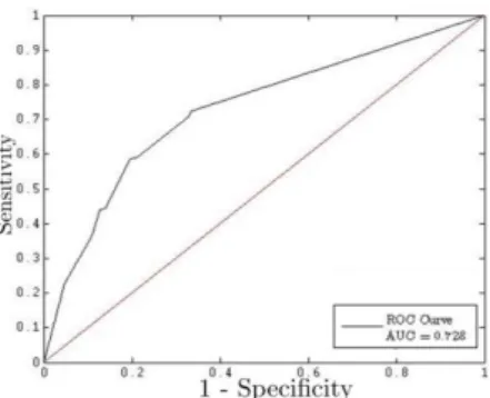
Due to the low number of error prone modules compared to the number of non error prone modules, other metrics such as AUC (Area Under ROC curve) are preferred[14]. The ROC (Receiver Operating Characteristics) curve is a two-dimensional plot of sensitivity versus (1 – specificity), Fig 2. The (0,1) point represents the optimal classifier, while random guessing results in a classifier located on the diagonal.

AUC has been previously adopted as an evaluation criterion in a number of

software defect prediction studies, e.g. [1][5][15]. In order to make our findings easier comparable to other studies, accuracy, sensitivity, and specificity are also reported.

Fig. 1: ROC curve (model trained on the KC1 data set, evaluated on the JM1 data set).

ROC analysis can only be applied in case of scoring classifiers (i.e. classifiers outputting a score which indicate the probability an instance belongs to a specific class). Rule sets are discrete by nature, providing only a dichotomous output. However, they can be converted into a scoring classifier following a number of approaches[14]. This can be typically done by creating multiple discrete classifiers and aggregating their output into a single score[16]. However, using such an ensemble method will result in an incomprehensible classifier.

Alternatively, a scoring classifier can be constructed by „looking inside‟ the classifier; in a rule set, each rule is characterized by its rule confidence, i.e. the number of modules correctly classified by a rule on a separate test set[17].

This rule confidence can be used as a score associated with each observation from the test set to construct the ROC curve. In case of smaller data sets, Laplace correction can be applied to the rule confidence to smooth the

predictions[18]. However, as the data sets are sufficiently large, this was not done.

4. Data Experiments

In this section, the data sets used in this study are introduced and the setup of the experiment is detailed. Subsequently, the empirical results are provided followed by a discussion of the results.

Table 1: Overview of data sets used in this study.

4.1. Data set characteristics

Table 1 provides an overview of the data sets used in this study. In total, twelve data sets are used to validate our approach. As can be seen from Table 1, the smallest data set contains 125 observations whereas the largest data set contains 10,878 observations. Each observation refers to a single software subroutine, function, or method. Thus, in the remainder of the paper, a software module refers to such a subroutine, function, or method, and is characterized by Lines Of Code (LOC) based metrics, Halstead metrics, and McCabe Complexity measures. The number of

defective modules is typically outnumbered by the non defective ones (last column). All data sets originate from the NASA MDP repository[3], and describe various space exploration related software projects such as flight software for an earth orbiting satellite (PC1 and PC4), a ground control system (KC1 and KC3), and NASA spacecraft system (CM1).

4.2. Experiment Design

CBA2 is compared to two other rule based classifiers, C4.5 rule[8] and RIPPER[9], across the 12 NASA MDP data sets. These techniques were selected as they are commonly used for software defect prediction.

The different classifiers are validated (in terms of accuracy, sensitivity, specificity, and AUC) by randomly splitting the data in test and training set. More specifically, 2/3 of the data is used to train the model while the induced model is validated on the remaining 1/3 of the data. The three classification techniques all exhibit adjustable parameters, also termed hyperparameters, which enable the adaptation of an algorithm to a specific problem. In the experiments, we adopted a grid-search approach to tune these hyperparameters.

That is, a set of candidate values is defined for each hyperparameter and all possible combinations are evaluated empirically by means of a 10-fold cross validation on the training data. The parameter combination resulting in the highest performance is retained and a classification model is constructed on the whole training set1.

1

In case of C4.5 and RIPPER, the parameter tuning was done by maximizing the AUC value, while in case of CBA2, accuracy was used as the CBA soft-ware package does not provide AUC values directly. Data set Attributes Modules Defects

CM1 39 505 48 (9.50%) JM1 21 10878 2102 (19.3%) KC1 21 2105 325 (15.4%) KC3 39 429 43 (10.0%) KC4 39 125 61 (48.8%) MC1 39 4621 68 (1.47%) MC2 39 161 52 (32.3%) MW1 39 403 31 (7.69%) PC1 39 1059 76 (7.18%) PC2 39 4505 23 (0.51%) PC3 39 1511 160 (10.6%) PC4 39 1347 178 (13.2%)

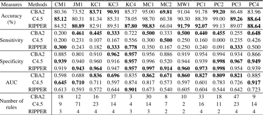
Table 2: Experimental results of CBA, C4.5 and RIPPER algorithms. The best performing classifier is indicated in bold face.

In addition, we assessed whether rule sets induced by the CBA2 classifier on a particular data set can be extrapolated towards other data sets. The twelve data sets were divided into two groups according to the number of attributes. For each group, we used the rule set derived from one data set to make predictions on other data sets. As such, we assessed the performance of the rule set on the other data sets. The results for this external validation will be discussed in the next section.

C4.5 and RIPPER classifiers are implemented using the WEKA software package[19]. As for the CBA2 classifier, the software is publicly available online at

http://www.comp.nus.edu.sg/~dm2/p_do wnload.html. The experiments were executed on a Windows XP based computer with Intel® Core 2 Duo™ 3.0 GHz processor with 3.0 Gb RAM.

4.3. Experimental Results

Table 2 presents the values of accuracy, sensitivity, specificity, AUC, and the number of rules for the different classifiers on the twelve data sets. As stated earlier, the analysis primarily

focuses on the AUC value for the different classifiers. For clarity, other metrics are also reported on.

We found that in most cases (i.e. 8 out 12), the CBA2 classifier is the best performing technique if looking at both AUC and sensitivity. In contrary, RIPPER outperforms the other techniques on most data sets as far as specificity is concerned.

In addition, we also tested the significance of these measurements‟ mean difference between any two algorithms by constructing a 95% confidence interval[20], Table 3. The testing results revealed that, on average, AUC and sensitivity values of CBA2 are significantly higher than for C4.5 and RIPPER. Furthermore, the accuracy of CBA2 was found to be not significantly different from that of C4.5 and RIPPER. In addition, the specificity of RIPPER was on average significantly higher than that of C4.5.

Focusing on specificity and sensitivity, we conclude that CBA2 performs better than C4.5 and RIPPER.

Focusing on the AUC values in Table 3, CBA2 performs better then the two other classification methods. We also found

Measures Methods CM1 JM1 KC1 KC3 KC4 MC1 MC2 MW1 PC1 PC2 PC3 PC4 Accuracy (%) CBA2 80.36 73.52 83.71 90.91 85.37 95.00 69.81 91.04 91.78 99.20 86.48 83.96 C4.5 85.12 80.31 81.34 85.31 78.05 98.70 60.38 90.30 88.39 99.00 89.26 88.64 RIPPER 84.52 80.89 82.91 89.51 87.80 98.83 66.04 91.79 92.07 99.13 89.07 88.64 Sensitivity CBA2 0.200 0.461 0.445 0.333 0.722 0.500 0.333 0.500 0.440 0.455 0.255 0.648 C4.5 0.200 0.231 0.107 0.167 0.556 0.300 0.500 0.250 0.160 0.000 0.235 0.426 RIPPER 0.300 0.243 0.182 0.333 0.778 0.350 0.167 0.250 0.240 0.091 0.333 0.500 Specificity CBA2 0.885 0.801 0.910 0.962 0.957 0.956 0.886 0.919 0.954 0.994 0.934 0.866 C4.5 0.939 0.940 0.960 0.916 0.957 0.996 0.520 0.944 0.939 0.998 0.967 0.949 RIPPER 0.919 0.943 0.964 0.947 0.957 0.997 0.914 0.960 0.973 0.998 0.954 0.939 AUC CBA2 0.598 0.688 0.836 0.696 0.835 0.862 0.671 0.860 0.827 0.809 0.821 0.885 C4.5 0.645 0.710 0.711 0.597 0.874 0.817 0.573 0.597 0.601 0.783 0.726 0.917 RIPPER 0.613 0.593 0.572 0.644 0.901 0.673 0.540 0.605 0.604 0.544 0.642 0.723 Number of rules CBA2 18 12 16 37 3 30 8 10 33 18 47 9 C4.5 9 71 23 14 4 14 7 2 16 11 23 14 RIPPER 3 4 4 4 3 3 2 2 4 2 4 4

that in most cases, the CBA2 classifier induces more rules than C4.5 and RIPPER. While we can observe an increase in AUC value in case of the CBA method, this apparently comes at the expense of a higher number of rules.

Measure Value Interval Significance

AUC CBA2-C4.5 [0.0051,0.1345] Yes CBA2-RIPPER [0.0751,0.2141] Yes

Accuracy CBA2-C4.5 [-2.79%,3.85%] No CBA2-RIPPER [-3.63%,0.29%] No

Sensitivity CBA2-C4.5 [0.0753,0.2847] Yes CBA2-RIPPER [0.0315,0.2227] Yes

Specificity CBA2-C4.5 [-0.0795,0.0791] No CBA2-RIPPER [-0.0629,-0.0107] Yes

Table 3: 95% confidence intervals on the mean difference for the AUC value of

different classifiers.

Data sets KC1 JM1 KC1 --- < JM1 < ---

Table 3: Results of global rule set of Group 1. Data sets CM1 KC3 KC4 MC1 MC2 MW1 PC1 PC2 PC3 PC4 CM1 --- > < < < < < < < < KC3 < --- < < > > < < > < KC4 < < --- < < < < < < < MC1 < < < --- < < < < < < MC2 < < < < --- < < < < < MW1 < < < < < --- < < < < PC1 < < < < < < --- < < < PC2 < < < < < < < --- < < PC3 < < < < < < < < --- < PC4 < < < < < < < < < ---

Table 4: Results of global rule set of Group 2.

Table 4 and 5 show the results of the external rule set validation. In each table, the horizontal names are the names of the

training set, while the vertical names are the data sets used for validation. As such, we compared the AUC value on a certain data set Di (AUCi) of Table 2 with the AUC value obtained by inducing the model on one data set and validating it on another (AUCj) using the CBA2 Classifier. If AUCj is less than AUCi, then the symbol “<” was entered in the corresponding cell of the table, else the symbol “>” was used.

From the results in Table 4 and 5, we observed that for all the 92 valid comparisons, only in four cases the “>” symbol was entered. This means that in most cases, the rule set derived from one particular data set by using the CBA2 classifier would yield a lower performance then a rule set induced on the same data set.

5. Conclusions and Future work

This paper has investigated the performance of an association rule based classification method for software defect prediction problems. Data experiments were conducted to compare the CBA2 classifier with two other rule/tree based classifiers (i.e. C4.5 and RIPPER), showing that the CBA2 method obtained satisfactory performance when compared to C4.5 and RIPPER, without losing comprehensibility.

Future studies could focus on comparing more classification methods and improving association rule based classification methods by using an AUC-based comparison framework for the domain of software defect prediction. Furthermore, the pruning of rules for association rule based classification methods will also be considered in our future work.

The work was partly supported by the National Natural Science Foundation of China (70890080), the MOE Project of Key Research Institute of Humanities and Social Sciences at Universities of China (7JJD63005), and Tsinghua-Leuven Research Cooperation Project (3H051154). We also extend our gratitude to the Flemish Research Fund for the financial support to the authors (Odysseus grant G.0915.09).

7. References

[1] C. Catal, and B. Diri, “A systematic re-view of software fault prediction studies,”

Expert Systems With applications, 36(4):7346-7354, 2009.

[2] C. Mair, M. Shepperd, and J. Magne, “An Analysis of Data Sets Used to Train and Validate Cost Prediction Systems,” ACM SIGSOFT Software Engineering Notes, 30(4):1-6, 2005.

[3] M. Chapman, P. Callis, and W. Jackson, “Metrics data programs,” Retrieved from

NASA IV and V facility:

http://mdp.ivv.nasa.gov, 2004.

[4] I. Gondra, “Applying machine learning to software fault-proneness prediction,” The Journal of Systems and Software, 81(2):186-195, 2008.

[5] S. Lessmann, B. Baesens, C. Mues, and S. Pietsch, “Benchmarking Classification Models For Software Prediction: A Pro-posed Framework and Novel Findings,”

IEEE Transactions on Software Engineer-ing, 34(4):485-496, 2008.

[6] G. Fung, S. Sandilya, and R.B. Rao, “Rule extraction form linear support vec-tor machines,” Proceedings of the ele-venth ACM SIGKDD International Confe-rence on Knowledge discovery in data mining, pp. 32-40, 2005.

[7] B. Liu, Y. Ma, C.K. Wong, “Improving an association rule based classifier,” In Proceedings of the Fourth European Con-ference on Principles and Practice of Knowledge Discovery in Databases (PKDD-2000), pp. 504-509, 2000.

[8]J.R. Quinlan, “C4.5: Programs for Machine Learning,” Morgan Kauf-man, 1993.

[9]W.W. Cohen, “Fast Effective Rule Induc-tion,” In: Twelfth International Confe-rence on Machine Learning, pp. 115-123, 1995.

[10]J.S. Shirabad, and T.J. Menzies, “The PROMISE Repository of Software Engi-neering Databases,” School of Informa-tion Technology and Eng., Univ. of Otta-wa,http://promise.site.uottawa.ca/SERepo sitory, 2005.

[11]R. Agrawal, and R. Srikant, “Fast algo-rithm for mining association rules,” Pro-ceeding of the 20th VLDB conference, pp. 487-499, 1994.

[12]B. Liu, W. Hsu, and Y. Ma, “Integrity classification and association rule min-ing,” Proceeding of the Fourth Interna-tional Conference on Knowledge Discov-ery and Data Mining, pp. 80-86, 1998. [13]D.G. Altman, and J.M. Bland,

“Diagnos-tic tests 1: Sensitivity and specificity,”

BMJ, 308, 1552, 1994.

[14]T. Fawcett, “An introduction to ROC analysis,” Pattern Recognition Letters, 27(8): 861–874, 2006.

[15]C. Catal, and B. Diri, “Investigating the effect of dataset size, metric sets, and fea-ture selection techniques on software fault prediction problem,” Information Sciences, 179(8):1040-1058, 2009. [16]L. Breiman, “Bagging predictors,”

Ma-chine Learning, 24(2):123-140, 1996. [17]I. Witten, and E. Frank, “Data mining:

Practical Machine Learning Tools and Techniques,” Morgan Kaufmann, 2005. [18]T. Fawcett, “Using Rule Sets to

Maxim-ize ROC Performance,” Proceedings of the 2001 IEEE International Conference on Data Mining, pp. 131-138, 2001. [19]S. Weiss, and C. Kulikowski, “Computer

Systems that Learn: Classification and Prediction Methods from Statistics, Neur-al Nets, Machine Learning, and Expert Systems,” Morgan Kaufman, 1991. [20] T.R. Harshbarger, “Introductory

Statistics: A Decision Map, Second edi-tion,” Macmillan Publishing Co., Inc. New York, Collier Macmillan Publishers, London, 1977.