A Reference Vector Guided Evolutionary Algorithm
for Many-objective Optimization
Ran Cheng, Yaochu Jin,
Fellow, IEEE
, Markus Olhofer and Bernhard Sendhoff,
Senior Member, IEEE
Abstract—In evolutionary multi-objective optimization, main-taining a good balance between convergence and diversity is particularly crucial to the performance of the evolutionary algorithms. In addition, it becomes increasingly important to incorporate user preferences because it will be less likely to achieve a representative subset of the Pareto optimal solutions using a limited population size as the number of objectives increases. This paper proposes a reference vector guided evolu-tionary algorithm for many-objective optimization. The reference vectors can not only be used to decompose the original multi-objective optimization problem into a number of single-multi-objective sub-problems, but also to elucidate user preferences to target a preferred subset of the whole Pareto front. In the proposed algo-rithm, a scalarization approach, termed angle penalized distance, is adopted to balance convergence and diversity of the solutions in the high-dimensional objective space. An adaptation strategy is proposed to dynamically adjust the distribution of the reference vectors according to the scales of the objective functions. Our experimental results on a variety of benchmark test problems show that the proposed algorithm is highly competitive in comparison with five state-of-the-art evolutionary algorithms for many-objective optimization. In addition, we show that reference vectors are effective and cost-efficient for preference articulation, which is particularly desirable for many-objective optimization. Furthermore, a reference vector regeneration strategy is pro-posed for handling irregular Pareto fronts. Finally, the propro-posed algorithm is extended for solving constrained many-objective optimization problems.
Index Terms—Evolutionary multiobjective optimization, refer-ence vector, many-objective optimization, convergrefer-ence, diversity, preference articulation, angle penalized distance
I. INTRODUCTION
M
ULTIOBJECTIVE optimization problems (MOPs),which involve more than one conflicting objective to be optimized simultaneously, can be briefly formulated as follows:
min
x f(x) = (f1(x), f2(x), ..., fM(x))
s.t. x∈X
(1)
where X ⊆ Rn is the decision space with x =
(x1, x2, ..., xn) ∈ X being the decision vector. Due to the
conflicting nature of the objectives, usually, there does not exist one single solution that is able to optimize all the
Ran Cheng and Yaochu Jin are with the Department of Computer Science, University of Surrey, Guildford, Surrey, GU2 7XH, United Kingdom (e-mail:{r.cheng;yaochu.jin}@surrey.ac.uk). Y. Jin is also with the College of Information Sciences and Technology, Donghua University, Shanghai 201620, P. R. China.
Markus Olhofer and Bernhard Sendhoff are with the Honda Research Institute Europe, 63073 Offenbach, Germany (e-mail:
{markus.olhofer;bernhard.sendhoff}@honda-ri.de).
objectives simultaneously. Instead, a set of optimal solutions representing the trade-offs between different objectives, termed Pareto optimal solutions, can be achieved. The Pareto optimal solutions are known as the Pareto front (PF) in the objective space and the Pareto set (PS) in the decision space, respec-tively.
Evolutionary algorithms (EAs), as a class of population based search heuristics, are able to obtain a set of solutions in a single run. Thanks to this attractive property, multiobjective evolutionary algorithms (MOEAs) have witnessed a boom of development over the past two decades [1]. MOEAs have been shown to perform well on a wide range of MOPs with two or three objectives; however, MOEAs have experienced substantial difficulties when they are adopted to tackle MOPs with more than three objectives [2]–[5], often referred to as the many-objective problems (MaOPs) nowadays. As a result, MaOPs have attracted increasing attention in evolutionary optimization [6].
One major reason behind the failure of most conventional MOEAs in solving MaOPs can be attributed to the loss of selection pressure, i.e., the pressure for the population to converge towards the PF, when dominance is adopted as a criterion for selecting individuals with a limited population size [7]. For example, the elitist non-dominated sorting genetic algorithm (NSGA-II) [8] and the strength Pareto evolutionary algorithm 2 (SPEA2) [9], both of which use dominance-based selection, will fail to work properly for MaOPs, since most candidate solutions generated in a population of a limited size are non-dominated, making the dominance based selection criterion hardly possible to distinguish the candidate solutions, even in a very early stage of the search.
Another important reason for the degraded performance of MOEAs on MaOPs is the difficulty in maintaining a good population diversity in a high-dimensional objective space. Generally speaking, since the PF of most continuous MOPs is piecewise continuous [10], [11], it is practically unlikely to approximate all Pareto optimal solutions. Instead, most MOEAs aim to find a set of evenly distributed representa-tive solutions to approximate the PF. When the number of objectives is two or three, where the PF is typically a one-dimensional curve or two-one-dimensional surface, maintaining a good diversity of the solutions is relatively straightforward. As the dimension of the objective space increases, it becomes in-creasingly challenging to maintain a good population diversity, as the candidate solutions distribute very sparsely in the high-dimensional objective space, causing immense difficulties to the diversity management strategies widely used in MOEAs, e.g., the crowding distance base diversity method in
NSGA-II [12]–[14].
To enhance the performance of most traditional MOEAs in solving MaOPs, a number of approaches have been pro-posed [15], [16], which can be roughly divided into three categories.
The first category covers various approaches to convergence enhancement. Since the loss of convergence pressure in most traditional MOEAs is directly caused by the inability of the canonical dominance to distinguish solutions, the most intuitive idea for convergence enhancement is to modify the dominance relationship to increase the selection pressure towards the PF. Examples of modified dominance definitions
include ϵ-dominance [17], [18],L-optimality [19], preference
order ranking [20] and fuzzy dominance [21]. In [22], a grid dominance based metric is defined for solving MaOPs, termed grid-based evolutionary algorithm (GrEA), which eventually modifies the dominance criterion to accelerate the convergence in many-objective optimization. Another typical idea in this category is to combine the Pareto dominance based criterion with additional convergence-related metrics. For example, K¨oppen and Yoshida [23] propose to use some substitute distances to describe the degree to which a solution almost dominates another to improve the performance of NSGA-II.
In [24], a binary ϵ-indicator based preference is combined
with dominance to speed up convergence of NSGA-II for solving MaOPs. In [25], a shift-based density estimation strategy is proposed to penalize poorly converged solutions by assigning them a high density value in addition to dominance comparison. In [26], a mating selection based on favorable convergence is applied to strengthen convergence pressure while an environmental selection based on directional diversity and favorable convergence is designed to balance diversity and convergence. In the recently proposed knee point driven evolutionary algorithm (KnEA) [27], a knee point based sec-ondary selection is designed on tope of non-dominated sorting to enhance convergence pressure.
The second category is often known as the decomposition based approaches, which divide a complex MOP into a number of sub-problems and solve them in a collaborative man-ner [28], [29]. There are mainly two types of decomposition based approaches [30]. In the first type of decomposition based approaches, an MOP is decomposed into a group of single-objective problems (SOPs), including the weighted aggregation based approaches in early days [31], [32], and the more recent multiobjective evolutionary algorithm based on decomposition (MOEA/D), where more explicit collaboration strategies between the solutions of the sub-problems were introduced. Several variants of MOEA/D have been proposed for enhancing the selection strategy for each sub-problem to strike a better balance between convergence and diversity [30], [33]–[37].
In the second type of decomposition based approaches, an MOP is decomposed into a group of sub-MOPs. For instance, MOEA/D-M2M [29], [38] divides the whole PF into a group of segments, and each segment can be regarded as a sub-problem. Another MOEA that essentially falls under this category is NSGA-III [39], where a set of predefined, evenly distributed reference points to manage the diversity
of the candidate solutions, eventually contribute to enhanced convergence of the algorithm. Although the second type of decomposition strategy has been reported very efficient in some recent works [40], [41], compared to the first type, its development is still in the infancy.
The third category is known as the performance indicator based approaches, e.g., the indicator based evolutionary al-gorithm (IBEA) [42], the S-metric selection based evolution-ary multi-objective algorithm (SMS-EMOA) [43], a dynamic neighborhood multi-objective evolutionary algorithm based on hypervolume indicator (DNMOEA/HI) [44], and the fast hypervolume based evolutionary algorithm (HypE) [45]. These approaches are not subject to the issues that dominance based MOEAs have for solving MaOPs. Unfortunately, the compu-tational cost for the calculation of the performance becomes prohibitively expensive when the number of objectives is large [46].
There are also a few approaches that do not fall into any of the above three main categories. For example, some researchers propose to use interactive user preferences [47] or reference points [48] during the search while others suggest to solve MaOPs by using a reduced set of objectives [49]– [51]. Another example is a recently proposed evolutionary many-objective optimization algorithm based on both domi-nance and decomposition (MOEA/DD) [41], the motivation of which is to exploit the merits offered by both dominance and decomposition based approaches. More recently, a two-archive algorithm for many-objective optimization (Two Arch2) has been proposed based on indicator and dominance [52].
While most existing MOEAs focusing on convergence en-hancement and diversity maintenance, it is noted that use of preferences will become particularly important for many-objective optimization, not only because the user may be interested in only part of Pareto optimal solutions, but also because it is less practical to achieve a representative subset of the whole PF using an evolutionary algorithm of a limited population size.
As already shown in [39], reference points can also be used to generate a subset of preferred Pareto optimal solutions, although NSGA-III can be seen as a decomposition based approach if the reference points are evenly distributed in the whole objective space. Motivated by ideas in decomposition based approaches and the aim to achieve the preferred part of the PF when the number of objectives is large, we propose a reference vector guided evolutionary algorithm (RVEA) for solving MaOPs. Compared with existing decomposition based approaches, the main new contributions of this work can be summarized as follows:
(1) A scalarization approach, termed as the angle penalized distance (APD), is designed to dynamically balance con-vergence and diversity in many-objective optimization according to the number of objectives and the number of generations. In the proposed APD, the convergence cri-terion is measured by the distance between the candidate
solutions and the ideal point1, and the diversity criterion
1For a minimization problem, the ideal point is a vector that consists of the minimum value of each objective function.
is measured by the acute angle between the candidate solutions and the reference vectors. Compared to the penalty-based boundary intersection (PBI) approach [28] that relies on the Euclidean distance, the angle-based distance metric makes it easier for normalization and is more scalable to the number of objectives, which is es-sential for many-objective optimization. Note that if the reference vectors are used to represent user preferences, this angle also indicates the degree of satisfaction of the user preferences.
(2) An adaptive strategy is proposed to adjust the refer-ence vectors to deal with objective functions that are not well normalized. The adaptive strategy adjusts the distribution of the reference vectors according to the ranges of different objective functions in order to ensure a uniform distribution of the candidate solutions in the objective space, even if the objective functions are not well normalized or the geometrical structure of a PF is highly asymmetric. This strategy is mainly for achieving an evenly distributed Pareto optimal subset.
(3) It is shown that reference vectors can also provide an effective and computationally efficient approach to preference articulation. Such preference articulation is particularly valuable in many-objective optimization, where it is very unlikely to obtain a representative approximation of the whole PF [53]. By specifying a central vector and a radius, we propose a reference vector based preference articulation approach that is able to generate evenly distributed Pareto optimal solutions in a preferred region in the objective space.
(4) To enhance the performance of the proposed RVEA
on problems with irregular2 Pareto fronts, a reference
vector regeneration strategy is proposed. The basic idea is to use an additional reference vector set to perform exploration in the objective space so that the density of the solutions obtained by RVEA on problems with irregular Pareto fronts can be improved.
(5) The proposed RVEA is further extended for solving constrained MaOPs.
The rest of this paper is organized as follows. Section II introduces some background knowledge. The details of the proposed RVEA are described in Section III. Section IV presents empirical results that compare the performance of RVEA with five state-of-the-art MOEAs for solving MaOPs. In addition, preference articulation using reference vectors is ex-emplified in Section V, a reference vector regeneration strategy for irregular Pareto fronts handling is presented in Section VI, and the extension of RVEA to handling constrained MaOPs is presented in Section VII. Finally, conclusions and future work are given in Section VIII.
II. BACKGROUND
In this section, we first present a brief review of decompo-sition based MOEAs. Then, an introduction to the reference vectors used in this work is given, including how to sample
2In this work, irregular Pareto fronts refer to disconnected and degenerate Pareto fronts.
uniformly distributed reference vectors and how to measure the spacial relationship between two vectors.
A. Decomposition based MOEAs
In weight aggregation based decomposition approaches, a
set ofweight vectorsare used to convert an MOP into a number
of SOPs using a scalarization method [28], [32], [54]. Among others, the weighted sum approach, the weighted Tchebycheff approach [55] and the PBI approach [28] are most widely used.
More recently, a set of weight vectors are used to divide an MOP into a number of sub-problems by partitioning the entire objective space into some subspaces, where each sub-problem remains an MOP. This type of decomposition strategy was
first proposed by Liu et al. in [29], where a set of direction
vectors are used to divide the whole PF into a number of segments, each segment being a multi-objective sub-problem. Such a decomposition strategy has attracted certain interests.
For example, in NSGA-III [39], a set of reference points or
reference lines are used for niche preservation to manage diversity in each subspace for many-objective optimization, which effectively enhances convergence by giving priority to solutions closer to the reference points. Most recently, an inverse model based MOEA (IM-MOEA) [40] has been
suggested, where a set ofreference vectorsare used to partition
the objective space into a number of subspaces and then in-verse models that map objective vectors onto decision vectors are built inside each subspace for sampling new candidate solutions.
Since weight vectors are typically used to denote the
importance of objectives in weighted aggregation, different terminologies have been coined in the second type of decom-position based approaches to refer to vectors that decompose
the original objective space, includingdirection vectors [29],
reference lines [39], and reference vectors [40]. In essence, these vectors play a similar role of partitioning the objective space into a number of subspaces. In this work, we adopt the term reference vectors.
When a set of evenly distributed reference vectors are generated for achieving representative solutions of the whole PF, the proposed RVEA can be considered as one of the second type of decomposition based approaches. However, if user preferences are available and a set of specific reference vectors are generated for achieving only a preferred section of the PF, RVEA can also be seen as a preference based approach. For example in [56], [57], a set of reference vectors have been used to achieve preferred subset of the Pareto-optimal solutions. In this sense, RVEA differs from most existing reference point based MOEAs [58]–[60] in that these algorithms use dominance and preference to search for preferred subset of the PF only. It is worth noting that there are other preference artic-ulation methods tailored for the decomposition based MOEAs.
For example in [61], Gonget al.have proposed an interactive
MOEA/D for multi-objective decision making. The idea is to dynamically adjust the distribution of the weight vectors according to the preferred region specified by a hypersphere.
search (LBS) [63] in MOEA/D to incorporate user preferences, where the preference information is specified by an aspiration point and a reservation point, together with a preference
neighborhood parameter. Most recently, Mohammadi et al.
have also proposed to integrate user preferences for many-objective optimization [64], where the preferred region is specified by a hypercube. These methods try to define some preferred regions and generate weight vectors inside them to guide the search of the MOEAs. The main difference between RVEA proposed in this work and the above methods lies in the fact that RVEA defines preferred regions using a central vector and a radius, and a new angle-based selection criterion is proposed.
B. Reference Vector
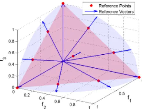
Fig. 1. An illustration of how to generate the uniformly distributed reference vectors in a three-objective space. In this case, 10 uniformly distributed reference points are first generated on a hyperplane, and then they are mapped to a hypersphere to generate the 10 reference vectors.
Without loss of generality, all the reference vectors used in this work are unit vectors inside the first quadrant with the origin being the initial point. Theoretically, such a unit vector can be easily generated via dividing an arbitrary vector by its norm. However, in practice, uniformly distributed unit reference vectors are required for a uniformly distributed coverage of the objective space. In order to generate uniformly distributed reference vectors, we adopt the approach intro-duced in [40]. Firstly, a set of uniformly distributed points on a unit hyperplane are generated using the canonical simplex-lattice design method [65]:
ui= (u1i, u 2 i, ..., u M i ), uji ∈ {0 H, 1 H, ..., H H}, M ∑ j=1 uji = 1, (2)
where i = 1, ..., N with N being the number of uniformly
distributed points, M is the objective number, and H is
a positive integer for the simplex-lattice design. Then, the
corresponding unit reference vectors vi can be obtained by
the following transformation:
vi=
ui
∥ui∥
, (3)
which maps the reference points from a hyperplane to a hyper-sphere, an example of which is shown in Fig. 1. According
to the property of the simplex-lattice design, given H and
M, a total number of N =(HM+M−1−1) uniformly distributed
reference vectors can be generated.
Given two vectorsv1andv2, the cosine value of the acute
angel θ between the two vectors can be used to measure
the spatial relationship between them, which is calculated as follows:
cosθ= v1·v2
∥v1∥∥v2∥
, (4)
where∥·∥calculates the norm, i.e., the length of the vector. As
will be introduced in the following section, in the proposed RVEA, (4) can be used to measure the spacial relationship between an objective vector and a reference vector in the objective space. Since they have already been normalized as in (2) when generated, the reference vectors no longer need to be normalized again in calculating the cosine values.
III. THE PROPOSEDRVEA
A. Elitism Strategy
Algorithm 1 The main framework of the proposed RVEA.
1: Input:the maximal number of generationstmax, a set of
unit reference vectors V0={v0,1,v0,2...,v0,N};
2: Output: final populationPtmax;
3: /*Initialization*/
4: Initialization: create the initial population P0 with N
randomized individuals; 5: /*Main Loop*/ 6: while t < tmax do 7: Qt = offspring-creation(Pt); 8: Pt=Pt∪Qt; 9: Pt+1 = reference-vector-guided-selection(t,Pt,Vt); 10: Vt+1 = reference-vector-adaptation(t,Pt+1,Vt,V0); 11: t=t+ 1; 12: end while
The main framework of the proposed RVEA is listed in Algorithm 1, from which we can see that RVEA adopts an elitism strategy similar to that of NSGA-II [8],where the offspring population is generated using traditional genetic operations such as crossover and mutation, and then the offspring population is combined with the parent population to undergo an elitism selection. The main new contributions in the RVEA lie in the two other components, i.e., the reference vector guided selection and the reference vector adaptation. In addition, RVEA requires a set of predefined reference vectors as the input, which can either be uniformly generated using (2) and (3), or specified according to the user preferences, which will be introduced in Section V. In the following subsections, we will introduce the three main components in Algorithm 1, i.e., offspring creation, reference vector guided selection and reference vector adaptation.
B. Offspring Creation
In the proposed RVEA, the widely used genetic operators, i.e., the simulated binary crossover (SBX) [66] and the poly-nomial mutation [67] are employed to create the offspring
population, as in many other MOEAs [22], [27], [28], [39], [45]. Here, we do not apply any explicit mating selection
strategy to create the parents; instead, givenN individuals in
the current population Pt, a number of⌊N/2⌋pair of parents
are randomly generated, i.e., each of theN individuals has an
equal probability to participate in the reproduction procedure. This is made possible partly thanks to the reference vector guided selection strategy, which is able to effectively manage the convergence and diversity inside small subspaces of the ob-jective space such that the individual inside each subspace can make an equal contribution to the population. Nevertheless, specific mating selection strategies can be helpful in solving problems having a multimodal landscape or a complex Pareto set [68].
C. Reference Vector Guided Selection
Similar to MOEA/D-M2M [29], [38], RVEA partitions the objective space into a number of subspaces using the reference vectors, and selection is performed separately inside each subspace. The objective space partition is equivalent to adding a constraint to the subproblem specified each reference vector, which is shown to be able to help balance the convergence and diversity in decomposition based approaches [69]. To be specific, the proposed reference vector guided selection strategy consists of four steps: objective value translation, population partition, angle penalized distance calculation and the elitism selection.
1) Objective Value Translation: According to the definition in Section II-B, the initial point of the reference vectors used in this work is always the coordinate origin. To be consistent with this definition, the objective values of the individuals in
population Pt, denoted as Ft = {ft,1,ft,2, ...,ft,|Pt|}, where
t is the generation index, are translated3 into F′
t via the
following transformation:
f′t,i=ft,i−zmint , (5)
where i = 1, ...,|Pt|, ft,i, f′t,i are the objective vectors
of individual i before and after the translation, respectively,
and zmin
t = (zt,min1 , zt,min2 , ..., zmint,m) represents the minimal
objective values calculated from Ft. The role of translation
operation is twofold: (1) to guarantee that all the translated objective values are inside the first quadrant, where the ex-treme point of each objective function is on the corresponding coordinate axis, thus maximizing the coverage of the reference vectors; (2) to set the ideal point to be the origin of the coordinate system, which will simplify the formulations to be presented later on. Some empirical results showing the significance of the objective value translation can be found in Supplementary Materials I.
2) Population Partition: After the translation of the
objec-tive values, populationPtis partitioned intoN subpopulations
Pt,1, Pt,2, ..., Pt,N by associating each individual with its
closest reference vector, referring to Fig. 2, where N is the
number of reference vectors. As introduced in Section II-B, the spacial relationship of two vectors is measured by the acute
3In Euclidean geometry, a translation is a rigid motion that moves every point a constant distance in a specified direction.
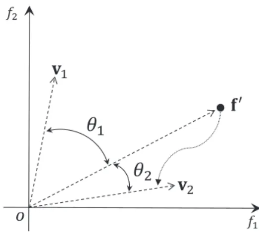
ߠ
ଵߠ
ଶ ݂ଶ ݂ଵܞ
ଵܞ
ଶ
Ԣ
Fig. 2. An example showing how to associate an individual with a reference vector. In this example,f′ is a translated objective vector,v1 and v2 are
two unit reference vectors.θ1andθ2are the angles betweenf′andv1,v2,
respectively. Sinceθ2< θ1, the individual denoted byf′is associated with
reference vectorv2.
angle between them, i.e., the cosine value between an objective vector and a reference vector can be calculated as:
cosθt,i,j=
f′t,i·vt,j ∥f′t,i∥
, (6)
whereθt,i,jrepresents the angle between objective vectorf′t,i
and reference vectorvt,j.
In this way, an individualIt,iis allocated to a subpopulation
Pt,kif and only if the angle betweenf′t,i andvt,kis minimal
(i.e., the cosine value is maximal) among all the reference vectors:
Pt,k={It,i|k= argmax j∈{1,...,N}
cosθt,i,j}, (7)
where It,i denotes the I-th individual in Pt, with i =
1, ...,|Pt|.
3) Angle-Penalized Distance (APD) Calculation: Once
the population Pt is partitioned into N subpopulations
Pt,1, Pt,2, ..., Pt,N, one elitist can be selected from each
subpopulation to create Pt+1 for the next generation.
Since our motivation is to find the solution on each reference vector that is closest to the ideal point, the selection criterion consists of two sub-criteria, i.e., the convergence criterion and the diversity criterion, with respect to the reference vector that the candidate solutions are associated with.
Specifically, given a translated objective vector f′t,i in
subpopulation j, the convergence criterion can be naturally
represented by the distance from f′t,i to the ideal point4,
i.e., ∥f′t,i∥; and the diversity criterion is represented by the
acute angle between f′t,i andvt,j, i.e., θt,i,j, as the inverse
function value of cosθt,i,j calculated in (6). In order to
balance between the convergence criterion ∥f′t,i∥ and the
diversity criterion θt,i,j, a scalarization approach, i.e., the
angle-penalized distance (APD)is proposed as follows: dt,i,j= (1 +P(θt,i,j))· ∥f′t,i∥, (8)
4As the objective values have been translated by subtracting the minimal value of each objective function in (5), the ideal point is always the coordinate origin. Therefore, the distance from a translated objective vector to the ideal point equals the norm (length) of the translated objective vector.
Algorithm 2The reference vector guided selection strategy in the proposed RVEA.
1: Input: generation index t, population Pt, unit reference
vector setVt={vt,1,vt,2, ...,vt,N};
2: Output: populationPt+1 for next generation;
3: /*Objective Value Translation*/
4: Calculate the minimal objective values zmint ;
5: fori= 1 to|Pt| do
6: f′t,i=ft,i−zmint ; //refer to (5)
7: end for 8: /*Population Partition*/ 9: fori= 1 to|Pt| do 10: forj = 1toN do 11: cosθt,i,j = f′t,i·vt,j ∥f′t,i∥ ; //refer to (6) 12: end for 13: end for 14: fori= 1 to|Pt| do 15: k= argmax j∈{1,...,N} cosθt,i,j; 16: Pt,k =Pt,k∪ {It,i}; //refer to (7) 17: end for
18: /*Angle-Penalized Distance (APD) Calculation*/
19: forj = 1toN do 20: fori= 1to|Pt,j|do
21: dt,i,j= (1 +P(θt,i,j))· ∥f′t,i∥; //refer to (8) (9) (10)
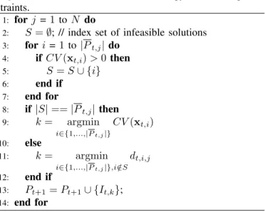
22: end for 23: end for 24: /*Elitism Selection*/ 25: forj = 1toN do 26: k= argmin i∈{1,...,|Pt,j|} dt,i,j; 27: Pt+1=Pt+1∪ {It,k}; 28: end for
withP(θt,i,j)being a penalty function related toθt,i,j:
P(θt,i,j) =M·( t tmax )α·θt,i,j γvt,j , (9) and γvt,j = min i∈{1,...,N},i̸=j⟨vt,i,vt,j⟩, (10)
where M is the number of objectives, N is the number of
reference vectors,tmax is the predefined maximal number of
generations,γvt,j is the smallest angle value between reference
vector vt,j and the other reference vectors in the current
generation, and αis a user defined parameter controlling the
rate of change ofP(θt,i,j). The detailed design of the penalty
function P(θt,i,j) in the APD calculation is based on the
following empirical observations.
Firstly, in many-objective optimization, since the candidate solutions are sparsely distributed in the high-dimensional objective space, it is not the best to apply a constant pressure on convergence and diversity in the entire search process. Ideally, at the early stage of the search process, a high selection pressure on convergence is exerted to push the population towards the PF, while at the late search stage, once the population is close to the PF, population diversity can be
emphasized in selection to generate well distributed candidate
solutions. The penalty function ,P(θt,i,j), is exactly designed
to meet these requirements. Specifically, at the early stage of
the search process (i.e, t ≪ tmax), P(θt,i,j) ≈ 0, and thus
dt,i,j ≈ ∥f′t,i∥ can be satisfied, which means that the value
of dt,i,j is mainly determined by the convergence criterion
∥f′t,i∥; while at the late stage of the search process, with the
value of t approaching tmax, the influence of P(θt,i,j) will
be gradually accumulated to emphasize the importance of the
diversity criterionθt,i,j.
Angleγvt,j is used to normalize the angles in the subspace
specified byvt,j. This angle normalization process is
particu-larly meaningful when the distribution of some reference vec-tors is either too dense (or too sparse), resulting in extremely small (or large) angles between the candidate solutions and the reference vectors. Compared to most existing objective normalization approaches, e.g., the one adopted in NSGA-III [39], the proposed angle normalization approach has two major differences: (1) normalizing the angles (instead of the objectives) will not change the actual positions of the candidate solutions, which is important convergence information for the proposed RVEA; (2) angle normalization, which is indepen-dently carried out inside each subspace, does not influence the distribution of the candidate solutions in other subspaces.
In addition, since the sparsity of the distribution of the candidate solutions is directly related to the dimension of the
objective space, i.e., the value of M, the penalty function
P(θt,i,j) is also related toM to adaptively adjust the range
of the penalty function values.
According to the angle penalized distances calculated using (8) and (9), the individual in each subpopulation having the minimal distance is selected as the elitist to be passed to the population for the next generation. The pseudo code of the reference vector guided selection procedure is summarized in Algorithm 2.
It is worth noting that the formulation of the proposed APD shares some similarity to PBI [28], which is widely adopted in the decomposition based MOEAs. However, there are two major differences between APD and PBI:
(1) In APD of the proposed RVEA, the angle between the reference vector and the solution vector is calculated for measuring diversity or the degree of satisfaction of the user preference, while in PBI, the Euclidean distance of the solution to the weight vector is calculated, which is a sort of diversity measure. Calculation of the difference in angle has certain advantages over calculation of the distance for the following two reasons. First, no matter what the exact distance a candidate solution is from the ideal point, the angle between the candidate solution and a reference vector is constant. Second, angles can be more easily normalized into the same range, e.g., [0, 1].
(2) The penalty itemP(θt,i,j)in APD is tailored for
many-objective optimization, which is adaptive to the search process as well as the number of objectives, while the
penalty item θ in PBI is a fixed parameter, which was
originally designed for multiobjective optimization. As pointed out in [70], there is no unique setting for the
of problems with different numbers of objectives. By contrast, our empirical results in Section IV demonstrate that APD works robustly well on a variety of problems with different numbers of objectives without changing
the setting for parameter α. This is mainly due to the
fact that the penalty function P(θt,i,j)in APD is able
to be normalized to a certain range, given any angles between the candidate solutions and the reference vector. Such a normalized penalty function provides a stable balancing between convergence and diversity, no matter whether the distribution of the reference vectors is sparse or dense.
Empirical results on comparing the proposed APD approach and the PBI approach can be found in Section IV-F.
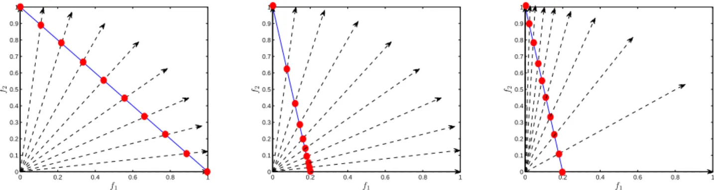
D. Reference Vector Adaptation
Given a set of uniformly distributed unit reference vectors, the proposed RVEA is expected to obtain a set of uniformly distributed Pareto optimal solutions that are the intersection points between each reference vector and the PF, as shown in Fig. 3(a). However, this happens only if the function values of all objectives can be easily normalized into the
same range, e.g., [0,1]. Unfortunately, in practice, there may
exist MaOPs where different objectives are scaled to different ranges, e.g., the WFG test problems [71] and the scaled DTLZ problems [39]. In this case, uniformly distributed reference vectors will not produce uniformly distributed solutions, as shown in Fig. 3(b).
One intuitive way to address the above issue is to carry out objective normalization dynamically as the search proceeds. Unfortunately, it turns out that objective normalization is not suited for the proposed RVEA, mainly due to the following reasons:
(1) Objective normalization, as a transformation that maps the objective values from a scaled objective space onto the normalized objective space, changes the actual ob-jective values, which will further influence the selection criterion, i.e., the angle penalized distance.
(2) Objective normalization has to be repeatedly performed as the scales of the objective values change in each generation.
As a consequence, performing objective normalization will cause instability in the convergence of the proposed RVEA due to the frequently changed selection criterion.
Nevertheless, it should be noted that although objective normalization is not suited for the proposed RVEA, it can work well for dominance based approaches such as NSGA-III, because the transformation does not change the partial orders, i.e., the dominance relations, between the candidate solutions, which is vital in dominance based approaches.
To illustrate the discussions above, we show below an empirical example. Given two translated objective vectors,
f′1 = (0.1,2) and f′2 = (1,10), where f′1 dominates f′2;
after objective normalization, the two vectors become f′1 =
(0.1,0.2)andf′2= (1,1). It can be seen that the dominance
relation is not changed, wheref′1still dominatesf′2. However,
the difference between the two vectors has been substantially
changed, from ∥f′2−f′1∥ = 8.0 to ∥f′2−f′1∥ = 1.2. It is
very likely such a substantial change will influence the results generated by the angle penalized distance in (8), thus causing instability in the selection process.
Therefore, instead of normalizing the objectives, we propose to adapt the reference vectors according to the ranges of the objective values in the following manner:
vt+1,i= v0,i◦(zmaxt+1 −zmint+1) ∥v0,i◦(zmaxt+1 −z min t+1)∥ , (11)
wherei= 1, ..., N,vt+1,i denotes the i-th adapted reference
vector for the next generation t+ 1, v0,i denotes the i-th
uniformly distributed reference vector, which is generated in
the initialization stage (on Line 1 in Algorithm 1), zmax
t+1
andzmin
t+1 denote the maximum and minimum values of each
objective function in the t+ 1 generation, respectively. The
◦operator denotes the Hadamard product that element-wisely
multiplies two vectors (or matrices) of the same size. With the reference vector adaptation strategy described above, the proposed RVEA will be able to obtain uniformly distributed solutions, even if the objective functions are not normalized to the same range, as illustrated in Fig. 3(c). Furthermore, some empirical results on the influence of the reference vector adaption strategy can be found in Appendix II.
Algorithm 3 The reference vector adaptation strategy in the proposed RVEA.
1: Input: generation index t, populationPt+1, current unit
reference vector setVt={vt,1,vt,2, ...,vt,N}, initial unit
reference vector setV0={v0,1,v0,2, ...,v0,N};
2: Output: reference vector setVt+1 for next generation; 3: if ( t
tmax modfr) == 0then
4: Calculate the minimal and maximal objective values
zmin
t+1 andzmaxt+1, respectively;
5: fori =1 toN do 6: vt+1,i= v0,i◦(zmaxt+1−zmint+1) ∥v0,i◦(ztmax+1−zmint+1)∥ ; //refer to (11); 7: end for 8: else 9: vt+1,i=vt,i; 10: end if
However, as pointed out by Giagkiozis et al. in [72], the
reference vector adaptation strategy should not be employed very frequently during the search process to ensure a stable convergence. Fortunately, unlike objective normalization, the reference vector adaptation does not have to be performed
in each generation. Accordingly, a parameter fr (Line 3
in Algorithm 3) is introduced to control the frequency of
employing the adaptation strategy. For instance, if fr is set
to0.2, the reference vector will only be adapted at generation
t= 0,t = 0.2×tmax,t = 0.4×tmax, t= 0.6×tmax and
t= 0.8×tmax, respectively. The detailed sensitivity analysis
of fr can be found in Supplementary Materials III.
Note that since the proposed reference vector adaptation strategy is only motivated to deal with problems with scaled objectives, it does not guarantee a uniform distribution of the reference vectors on any type of PFs, especially on
0 0.2 0.4 0.6 0.8 1 0 0.1 0.2 0.3 0.4 0.5 0.6 0.7 0.8 0.9 1 f1 f2
(a) Pareto optimal solutions specified by 10 uni-formly distributed reference vectors on a PF with objectives normalized to the same range.
0 0.2 0.4 0.6 0.8 1 0 0.1 0.2 0.3 0.4 0.5 0.6 0.7 0.8 0.9 1 f1 f2
(b) Pareto optimal solutions specified by 10 uni-formly distributed reference vectors on a PF with objectives scaled different ranges.
0 0.2 0.4 0.6 0.8 1 0 0.1 0.2 0.3 0.4 0.5 0.6 0.7 0.8 0.9 1 f1 f2
(c) Pareto optimal solutions specified by 10 adapted reference vectors on a PF with objectives scaled to different ranges.
Fig. 3. The Pareto optimal solutions (solid dots) specified by different reference vectors (dashed arrows) on different PF (solid lines).
those with irregular geometrical features, e.g., disconnection or degeneration. In order to handle such irregular PFs, we have proposed another reference vector regeneration strategy in Section VI. Nevertheless, it is conceded that the proposed reference vector adaptation (as well as regeneration) strategy is not able to comfortably handle all specific situations, e.g., when a PF has low tails or sharp peaks [73].
E. Computational Complexity of the Proposed RVEA
To analyze the computational complexity of the proposed RVEA, we consider the main steps in one generation in the main loop of Algorithm 1. Apart from genetic operations such as crossover and mutation, the main computational cost is resulted from the reference vector guided selection procedure and the reference vector adaptation mechanism.
As shown in Algorithm 2, the reference vector guided selection procedure consists of the following components: ob-jective value translation, population partition, angle-penalized distance (APD) calculation and elitism selection. We will see that the computational complexity of each component is very low, as will be analyzed in the following. The time complexity
for the objective value translation is O(M N), where M is
the objective number and N is the population size. The time
complexity for population partition is O(M N2). In addition,
calculation of APD and elitism selection hold a computational
complexity ofO(M N2)andO(N2)in the worst case,
respec-tively. Finally, the computational complexity for the reference
vector adaptation procedure is O(M N/(fr· tmax)), where
fr and tmax denote the frequency to employ the reference
vector adaptation strategy and maximal number of generations, respectively.
To summarize, apart from the genetic variations, the worst-case overall computational complexity of RVEA within one
generation is O(M N2), which indicates that RVEA is
com-putationally efficient.
IV. COMPARATIVE STUDIES
In this section, empirical experiments are conducted on 15 benchmark test problems taken from two widely used test
suites, i.e., the DTLZ [74] test suite (including the scaled ver-sion [39]) and the WFG test suite [71], to compare RVEA with five state-of-the-art MOEAs for many-objective optimization, namely, MOEA/DD [41], NSGA-III [39], MOEA/D-PBI [28], GrEA [22], and KnEA [27]. For each test problem, objective
numbers varying from 3 to 10, i.e., M ∈ {3,6,8,10} are
considered.
In the following subsections, we first present a brief in-troduction to the benchmark test problems and the perfor-mance indicator used in our comparative studies. Then, the parameter settings used in the comparisons are given. Then, each algorithm is run for 20 times on each test problem independently, and the Wilcoxon rank sum test is adopted to compare the results obtained by RVEA and those by five compared algorithms at a significance level of 0.05. Symbol
’+’ indicates that the compared algorithm is significantly
outperformed by RVEA according to a Wilcoxon rank sum
test, while ’−’ means that RVEA is significantly outperformed
by the compared algorithm. Finally, ’≈’ means that there is no
statistically significant difference between the results obtained by RVEA and the compared algorithm.
A. Benchmark Test Problems
The first four test problems are DTZL1 to DTLZ4 taken from the DTLZ test suite [74]. As recommended in [74], the
number of decision variables is set ton=M+K−1, where
M is the objective number,K= 5is used for DTLZ1,K= 10
is used for DTLZ2, DTLZ3 and DTLZ4.
We have also used the scaled version of the DTLZ1 and DTLZ3 (denoted as SDTLZ1 and SDTLZ3) for compar-isons to see if the proposed RVEA is capable of handling strongly scaled problems. The scaling approach is recom-mended in [39], where each objective is multiplied by a
coefficient pi−1, where p is a parameter that controls the
scaling size and i = 1, .., M is the objective index. For
example, givenp= 10, the objectives of a 3-objective problem
will be scaled to be100×f
1,101×f2 and102×f3. In our
experiments, the values ofpare set to10,5,3,2for problems
with an objective numberM = 3,6,8,10, respectively .
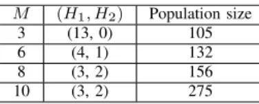
TABLE I
SETTINGS OF POPULATION SIZES INRVEA, MOEA/DD, NSGA-IIIAND
MOEA/D-PBI. M (H1, H2) Population size 3 (13, 0) 105 6 (4, 1) 132 8 (3, 2) 156 10 (3, 2) 275
H1andH2are the the simplex-lattice design factors for generating uniformly
distributed reference (or weight) vectors on the outer boundaries and the inside layers, respectively.
from the WFG test suite [71], [75], which are designed by introducing difficulties in both the decision space (e.g. non-separability, deception and bias) and the objective space (e.g. mixed geometrical structures of the PFs). As suggested in [71],
the number of decision variables is set as n =K+L−1,
whereM is the objective number, the distance-related variable
L = 10is used in all test problems, and the position-related
variableK= 4,10,7,9are used for test problems withM =
3,6,8,10, respectively.
B. Performance Indicators
To make empirical comparisons between the results ob-tained by each algorithm, the hypervolume (HV) [46] is used as the performance indicator in the comparisons.
Let y∗= (y∗1, ..., yM∗ )be a reference point in the objective
space that is dominated by all Pareto optimal solutions, andP
be the approximation to PF obtained by an MOEA. The HV
value of P (with respect to y∗) is the volume of the region
which dominates y∗ and is dominated byP.
In this work, y∗ = (1.5,1.5, ...,1.5) is used for DTLZ1,
SDTLZ1; y∗ = (2,2, ...,2) is used for DTLZ2, DTLZ3,
SDTLZ3, DTLZ4; and y∗ = (3,5, ...,2M + 1) is used for
WFG1 to WFG9. For problems with fewer than 8 objectives, the recently proposed fast hypervolume calculation method is adopted to calculate the exact hypervolume [76], while for 8-objective and 10-objective problems, the Monte Carlo method [43] with 1,000,000 sampling points is adopted to obtain the approximate hypervolume values. All hypervolume
values presented in this work are all normalized to [0,1] by
dividing ∏mi=1yi∗.
C. Parameter Settings
In this subsection, we first present the general parameter settings for the experiments, and afterwards, the specific parameter settings for each algorithm in comparison are given.
1) Settings for Crossover and Mutation Operators: For the simulated binary crossover [66], the distribution index is set to
ηc= 30in RVEA, MOEA/DD and NSGA-III,ηc = 20in the
other four algorithms, and the crossover probability pc = 1.0
is used in all algorithms; for the polynomial mutation [67], the
distribution index and the mutation probability are set toηm=
20 andpm= 1/n, respectively, as recommended in [77].
2) Population Size: For RVEA, MOEA/DD, NSGA-III and MOEA/D-PBI, the population size is determined by the
simplex-lattice design factor H together with the objective
TABLE II
PARAMETER SETTING OFdivINGREAON EACH TEST INSTANCE
Problem M = 3 M = 4 M = 6 M = 8 M = 10 DTLZ1 16 10 10 10 11 DTLZ2 15 10 10 8 12 DTLZ3 17 11 11 10 11 DTLZ4 15 10 8 8 12 SDTLZ1 16 10 10 10 11 SDTLZ3 17 11 11 10 11 WFG1 10 8 9 7 10 WFG2 12 11 11 11 11 WFG3 22 18 18 16 22 WFG4–9 15 10 9 8 12 TABLE III
PARAMETER SETTING OFT INKNEAON EACH TEST INSTANCE
Problem M = 3 M = 4 M = 6 M = 8 M = 10 DTLZ1 0.6 0.6 0.2 0.1 0.1 DTLZ3 0.6 0.4 0.2 0.1 0.1 SDTLZ1 0.6 0.6 0.2 0.1 0.1 SDTLZ3 0.6 0.4 0.2 0.1 0.1 others 0.5 0.5 0.5 0.5 0.5
numberM, referring to (2). As recommended in [39], [41], for
problems withM ≥8, a two-layer vector generation strategy
can be applied to generate reference (or weight) vectors not only on the outer boundaries but also on the inside layers of the Pareto fronts. The detailed settings of the population sizes in RVEA, MOEA/DD, NSGA-III and MOEA/D-PBI are summarized in Table I. For the other two algorithms, GrEA and KnEA, the population sizes are also set according to
Table I, with respect to different objective numbers M.
3) Termination Condition: The termination condition of each run is the maximal number of generations. For DTLZ1, SDTLZ1, DTLZ3, SDTLZ3 and WFG1 to WFG9, the max-imal number of generations is set to 1000. For DTLZ2 and DTLZ4, the maximal number of generations is set to 500.
4) Specific Parameter Settings in Each Algorithm: For
MOEA/D-PBI, the neighborhood sizeT is set to20, and the
penalty parameterθin PBI is set to 5, as recommended in [28],
[39]. For MOEA/DD, T andθ are set to the same values as
in MOEA/D-PBI, and the neighborhood selection probability
is set to δ = 0.9, as recommended in [41]. For GrEA and
KnEA, the detailed parameter settings are listed in Table II and Table III, respectively, which are all recommended settings by the authors [22], [27].
Two parameters in RVEA require to be predefined, i.e., the
index α used to control the rate of change of the penalty
function in (9), and the frequencyfrto employ the reference
vector adaptation in Algorithm 3. In the experimental
compar-isons, α= 2 and fr = 0.1 is used for all test instances. A
sensitivity analysis ofαandfr is provided in Supplementary
Materials III.
In order to reduce the time cost of non-dominated sort-ing, the efficient non-dominated sorting approach ENS-SS reported in [78] has been adopted in NSGA-III, GrEA and KnEA, and a steady-state non-dominated sorting approach as reported in [79] has been adopted in MOEA/DD. By contrast, neither RVEA nor MOEA/D-PBI uses dominance
compar-isons. All the algorithms are realized in Matlab R2012a5
except MOEA/DD, which is implemented in the jMetal frame-work [80]. D. Performance on DTLZ1 to DTLZ4, SDTLZ1 and SDTLZ3 1 2 3 4 5 6 7 8 9 10 0 0.1 0.2 0.3 0.4 0.5 0.6 0.7 Objective Number Objective Value (a) RVEA 1 2 3 4 5 6 7 8 9 10 0 0.1 0.2 0.3 0.4 0.5 0.6 0.7 Objective Number Objective Value (b) MOEA/DD 1 2 3 4 5 6 7 8 9 10 0 0.1 0.2 0.3 0.4 0.5 0.6 0.7 Objective Number Objective Value (c) NSGA-III 1 2 3 4 5 6 7 8 9 10 0 0.1 0.2 0.3 0.4 0.5 0.6 0.7 Objective Number Objective Value (d) MOEA/D-PBI 1 2 3 4 5 6 7 8 9 10 0 20 40 60 80 100 120 140 160 180 Objective Number Objective Value (e) GrEA 1 2 3 4 5 6 7 8 9 10 0 50 100 150 200 250 300 350 Objective Number Objective Value (f) KnEA Fig. 4. The parallel coordinates of non-dominated front obtained by each algorithm on 10-objective DTLZ1 in the run associated with the median HV value. 1 2 3 4 5 6 7 8 9 10 0 0.2 0.4 0.6 0.8 1 1.2 1.4 Objective Number Objective Value (a) RVEA 1 2 3 4 5 6 7 8 9 10 0 0.2 0.4 0.6 0.8 1 1.2 1.4 Objective Number Objective Value (b) MOEA/DD 1 2 3 4 5 6 7 8 9 10 0 0.2 0.4 0.6 0.8 1 1.2 1.4 Objective Number Objective Value (c) NSGA-III 1 2 3 4 5 6 7 8 9 10 0 0.2 0.4 0.6 0.8 1 1.2 1.4 Objective Number Objective Value (d) MOEA/D-PBI 1 2 3 4 5 6 7 8 9 10 0 0.2 0.4 0.6 0.8 1 1.2 1.4 Objective Number Objective Value (e) GrEA 1 2 3 4 5 6 7 8 9 10 0 0.2 0.4 0.6 0.8 1 1.2 1.4 Objective Number Objective Value (f) KnEA Fig. 5. The parallel coordinates of non-dominated front obtained by each algorithm on 10-objective DTLZ4 in the run associated with the median HV value.
The statistical results of the HV values obtained by the six algorithms over 20 independent runs are summarized in Table IV, where the best results are highlighted. It can be seen that RVEA, together with MOEA/DD, shows best overall performance among the six compared algorithms on the four original DTLZ test instances, while NSGA-III shows the best overall performance on the scaled DTLZ test instances.
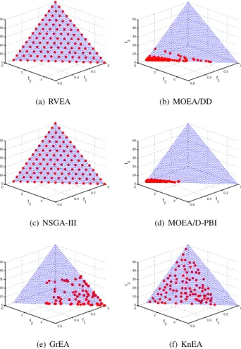
As can be observed from Fig. 4, the approximate PFs ob-tained by RVEA, MOEA/DD and MOEA/D-PBI show promis-ing convergence performance as well as a good distribution on 10-objective DTLZ1. The statistical results in Table IV
5The Matlab source code of RVEA can be downloaded from: http://www.soft-computing.de/jin-pub year.html 0 0.2 0.4 0.6 0 2 4 0 10 20 30 40 50 f1 f2 f3 (a) RVEA 0 0.2 0.4 0.6 0 2 4 0 10 20 30 40 50 f1 f2 f3 (b) MOEA/DD 0 0.2 0.4 0.6 0 2 4 0 10 20 30 40 50 f1 f2 f3 (c) NSGA-III 0 0.2 0.4 0.6 0 2 4 0 10 20 30 40 50 f 1 f2 f3 (d) MOEA/D-PBI 0 0.2 0.4 0.6 0 2 4 0 10 20 30 40 50 f1 f2 f3 (e) GrEA 0 0.2 0.4 0.6 0 2 4 0 10 20 30 40 50 f1 f2 f3 (f) KnEA
Fig. 6. The non-dominated solutions obtained by each algorithm on 3-objective SDTLZ1 in the run associated with the median HV value.
also indicate that RVEA, MOEA/DD and MOEA/D-PBI have achieved the best performance among the six algorithms on all DTLZ1 instances, where MOEA/DD shows best performance on 3-objective instance and RVEA shows best performance on 6-objective and 8-objective instances. Meanwhile, the PFs approximated by NSGA-III is also of high quality. By contrast, neither GrEA nor KnEA is able to converge to the true PF of 10-objective DTLZ1.
Similar observations can be made about the results on DTLZ2, a relatively simple test problem, to those on DTLZ1. RVEA shows the best performance on the 8-objective instance, while MOEA/DD outperforms RVEA on 3-objective and 6-objective instances. NSGA-III and MOEA/D-PBI are slightly outperformed by RVEA. Compared to the performance on 10-objective DTLZ1, the performance of GrEA and KnEA on this instance is much better.
For DTLZ3, which is a highly multimodal problem, RVEA and MOEA/DD have also obtained an approximate PF of high quality. It seems that the performance of NSGA-III and MOEA/D-PBI is not very stable on high dimensional (8-objective and 10-objective) instances of this problem, as evidenced by the statistical results in Table IV, while GrEA and KnEA completely fail to reach the true PF of this problem. DTLZ4 is test problem where the density of the points on the true PF is strongly biased. This test problem is designed to verify whether an MOEA is able to maintain a proper
TABLE IV
THE STATISTICAL RESULTS(MEAN AND STANDARD DEVIATION)OF THEHVVALUES OBTAINED BYRVEA, MOEA/DD, NSGA-III, MOEA/D-PBI, GREAANDKNEAONDTLZ1TODTLZ4, SDTLZ1ANDSDTLZ3. THE BEST RESULTS ARE HIGHLIGHTED.
Problem M RVEA MOEA/DD NSGA-III MOEA/D-PBI GrEA KnEA
DTLZ1 3 0.992299 (0.000027) 0.992321 (0.000005)− 0.992275 (0.000017)+ 0.992217 (0.000068)+ 0.951715 (0.053104)+ 0.961327 (0.022927)+ 6 0.999966 (0.000021) 0.999965 (0.000017)≈ 0.999951 (0.000060)≈ 0.999969 (0.000007)≈ 0.806853 (0.101147)+ 0.902769 (0.064009)+ 8 0.999999 (0.000000) 0.999984 (0.000016)+ 0.999993 (0.000022)+ 0.999998 (0.000001)+ 0.949778 (0.081134)+ 0.774819 (0.054991)+ 10 0.999999 (0.000000) 0.999995 (0.000005)+ 0.999992 (0.000027)≈ 0.999999 (0.000000)≈ 0.950476 (0.088517)+ 0.906688 (0.070628)+ DTLZ2 3 0.926994 (0.000041) 0.927292 (0.000002)− 0.927012 (0.000032)≈ 0.926808 (0.000042)+ 0.926675 (0.000122)+ 0.925387 (0.000225)+ 6 0.995935 (0.000175) 0.996096 (0.000146)− 0.995689 (0.000062)+ 0.995872 (0.000078)≈ 0.996049 (0.000141)≈ 0.995249 (0.000250)+ 8 0.999338 (0.000096) 0.999330 (0.000079)≈ 0.998223 (0.002551)+ 0.999333 (0.000024)+ 0.999059 (0.000065)+ 0.999104 (0.000119)+ 10 0.999912 (0.000040) 0.999920 (0.000022)≈ 0.999804 (0.000222)+ 0.999917 (0.000011)+ 0.999921 (0.000022)≈ 0.999841 (0.000209)+ DTLZ3 3 0.924421 (0.001273) 0.926921 (0.000316)− 0.925650 (0.000664)+ 0.924153 (0.001546)+ 0.869279 (0.120728)+ 0.894023 (0.041540)+ 6 0.995596 (0.000228) 0.995848 (0.000203)− 0.768098 (0.402591)+ 0.970814 (0.077681)+ 0.592477 (0.120285)+ 0.523015 (0.073019)+ 8 0.999350 (0.000090) 0.999338 (0.000069)≈ 0.683011 (0.452841)+ 0.997552 (0.004021)+ 0.249152 (0.262630)+ 0.596495 (0.129071)+ 10 0.999919 (0.000027) 0.999914 (0.000033)≈ 0.588230 (0.507488)+ 0.883623 (0.195053)+ 0.173715 (0.287635)+ 0.665098 (0.163428)+ DTLZ4 3 0.926922 (0.000049) 0.927295 (0.000001)− 0.926947 (0.000035)≈ 0.761109 (0.188313)+ 0.913877 (0.040960)+ 0.925410 (0.000274)+ 6 0.995886 (0.000218) 0.995972 (0.000150)≈ 0.992253 (0.008107)+ 0.958608 (0.028688)+ 0.995811 (0.000204)≈ 0.995341 (0.000240)+ 8 0.999359 (0.000043) 0.999374 (0.000057)≈ 0.999016 (0.000055)+ 0.987237 (0.013487)+ 0.999164 (0.000079)+ 0.999181 (0.000041)+ 10 0.999915 (0.000036) 0.999916 (0.000019)≈ 0.999844 (0.000023)+ 0.998947 (0.000615)+ 0.999921 (0.000031)≈ 0.999904 (0.000014)≈ SDTLZ1 3 0.942902 (0.000374) 0.842188 (0.000255)+ 0.943320 (0.000258)− 0.752965 (0.026594)+ 0.811754 (0.135200)+ 0.890970 (0.020920)+ 6 0.987277 (0.005948) 0.825625 (0.005232)+ 0.994307 (0.004067)− 0.784053 (0.009784)+ 0.787636 (0.148348)+ 0.822863 (0.119886)+ 8 0.977781 (0.013207) 0.918495 (0.004078)+ 0.994885 (0.005614)− 0.879281 (0.008595)+ 0.603896 (0.285257)+ 0.638502 (0.124225)+ 10 0.997845 (0.003597) 0.968728 (0.005022)+ 0.999669 (0.000593)− 0.961194 (0.002466)+ 0.699631 (0.172086)+ 0.784741 (0.125824)+ SDTLZ3 3 0.728992 (0.004089) 0.611762 (0.005177)+ 0.731667 (0.002343)≈ 0.510602 (0.018017)+ 0.704035 (0.063554)+ 0.687029 (0.038566)+ 6 0.645483 (0.099350) 0.628237 (0.011612)+ 0.694999 (0.360772)− 0.545299 (0.002836)+ 0.008744 (0.027535)+ 0.003786 (0.009766)+ 8 0.673466 (0.071693) 0.667774 (0.005031)+ 0.337208 (0.378458)+ 0.556130 (0.000727)+ 0.057487 (0.119544)+ 0.370506 (0.213103)+ 10 0.869416 (0.044609) 0.573527 (0.005793)+ 0.753836 (0.397503)+ 0.727759 (0.004431)+ 0.018452 (0.019051)+ 0.470806 (0.187499)+ +: RVEA shows significantly better performance in the comparison.
−: RVEA shows significantly worse performance in the comparison.
≈: There is no significant difference between the compared results.
distribution of the candidate solutions. From the results, we can see that RVEA and MOEA/DD remain to show the best overall performance. By contrast, MOEA/D-PBI is generally outperformed by the other five algorithms. As can be observed from Fig. 5, it appears that MOEA/D-PBI is only able to find some parts of the true PF. The performance of NSGA-III is similar to that of RVEA. An interesting observation is that, although the distribution of the approximate PFs obtained by GrEA and KnEA look slightly noisy, the solutions are still relatively evenly distributed, and thus the HV values obtained by these two algorithms are very encouraging, especially on the 8-objective and 10-objective instances.
Compared with the original DTLZ problems, the SDTLZ1 and SDTLZ3 are challenging due to the strongly scaled objec-tive function values. It turns out that NSGA-III shows the best overall performance on SDTLZ1, 3-objective and 6-objective SDTLZ3, while RVEA shows the best overall performance on 8-objective and 10-objective SDTLZ3. As shown in Fig. 6, RVEA and NSGA-III are the only two algorithms that are able to generate evenly distributed solutions on the 3-objective SDTLZ1, while the other four algorithms have all failed. Such observations are consistent with those reported in [39], where it has been shown that even the normalized version of MOEA/D still does not work on such scaled DTLZ problems.
E. Performance on WFG1 to WFG9
As evidenced by statistical results of the HV values sum-marized in Table V, RVEA has shown the most competitive
performance on WFG4, WFG5, WFG6, WFG7 and WFG9, while MOEA/DD, NSGA-III, GrEA and GrEA have achieved the best performance on WFG8, WFG2, WFG3 and WFG1, respectively. By contrast, the performance of MOEA/D-PBI on the WFG test functions is not as good as that on the DTLZ test functions. In the following, some discussions on the experimental results will be presented.
WFG1 is designed with flat bias and a mixed structure of the PF. Although RVEA is slightly outperformed by GrEA and KnEA, its performance is still significantly better than NSGA-III and MOEA/D-PBI. WFG2 is a test problem which has a disconnected PF. It can be observed that although the HV val-ues obtained by each algorithm vary on this test problem, the overall performance is generally very good. More specifically, the overall performance of RVEA is better than MOEA/D-PBI and GrEA, while NSGA-III has achieved the best overall performance. WFG3 is a difficult problem where the PF is degenerate and the decision variables are non-separable. On this problem, RVEA has achieved comparable higher HV values than MOEA/D-PBI, but has been outperformed by the other four algorithms, where GrEA has achieved the largest HV values on all the instances of this problem.
WFG4 to WFG9 are designed with different difficulties in the decision space, e.g., multimodality for WFG4, landscape deception for WFG5 and non-separability for WFG6, WFG8 and WFG9, though the true PFs are of the same convex structure. As can be observed in Table V, RVEA shows the most competitive overall performance on these six problems
TABLE V
THE STATISTICAL RESULTS(MEAN AND STANDARD DEVIATION)OF THEHVVALUES OBTAINED BYRVEA, MOEA/DD, NSGA-III, MOEA/D-PBI, GREAANDKNEAONWFG1TOWFG9. THE BEST RESULTS ARE HIGHLIGHTED.
Problem M RVEA MOEA/DD NSGA-III MOEA/D-PBI GrEA KnEA
WFG1 3 0.865072 (0.044144) 0.853637 (0.014545)≈ 0.880642 (0.037913)≈ 0.808559 (0.039850)+ 0.948634 (0.004706)− 0.958812 (0.003336)− 6 0.838645 (0.052536) 0.847766 (0.036001)≈ 0.760115 (0.030498)+ 0.937861 (0.034231)+ 0.978189 (0.002217)− 0.987990 (0.021758)− 8 0.828420 (0.071859) 0.874047 (0.029795)≈ 0.636388 (0.041800)+ 0.873566 (0.084635)≈ 0.984504 (0.003077)− 0.993004 (0.003330)− 10 0.912619 (0.059865) 0.862892 (0.004600)+ 0.570728 (0.048639)+ 0.802624 (0.118040)+ 0.989678 (0.002609)− 0.995399 (0.003227)− WFG2 3 0.911168 (0.070014) 0.911115 (0.070477)≈ 0.913209 (0.069967)≈ 0.850708 (0.072264)+ 0.907856 (0.069149)≈ 0.941823 (0.046468)− 6 0.929838 (0.084468) 0.969481 (0.004744)≈ 0.974124 (0.058171)− 0.824505 (0.068663)+ 0.959854 (0.055499)≈ 0.992704 (0.000971)− 8 0.985362 (0.002434) 0.964892 (0.005227)+ 0.995848 (0.001354)− 0.952490 (0.002702)+ 0.974283 (0.002684)+ 0.994149 (0.000685)− 10 0.990577 (0.002493) 0.962456 (0.004293)+ 0.997515 (0.000882)− 0.953995 (0.001703)+ 0.984013 (0.002625)+ 0.995553 (0.000637)− WFG3 3 0.548860 (0.008423) 0.547597 (0.003333)≈ 0.571840 (0.003352)− 0.536581 (0.023869)≈ 0.581615 (0.001209)− 0.572039 (0.005376)− 6 0.146476 (0.033719) 0.193116 (0.016724)− 0.324412 (0.026666)− 0.120196 (0.030687)≈ 0.375592 (0.001591)− 0.218213 (0.038518)− 8 0.022206 (0.028688) 0.092131 (0.011635)− 0.165832 (0.045706)− 0.001958 (0.003823)+ 0.299918 (0.002411)− 0.172217 (0.027005)− 10 0.010805 (0.015590) 0.049190 (0.009707)− 0.103724 (0.050683)− 0.000000 (0.000000)+ 0.277491 (0.001015)− 0.124849 (0.023234)− WFG4 3 0.722421 (0.001194) 0.727762 (0.000320)− 0.716893 (0.002451)+ 0.693973 (0.006281)+ 0.727825 (0.000843)− 0.718904 (0.001444)+ 6 0.862869 (0.008112) 0.884741 (0.001449)− 0.822742 (0.035516)+ 0.685602 (0.031404)+ 0.865653 (0.004690)≈ 0.854176 (0.003003)+ 8 0.931277 (0.001998) 0.905293 (0.005383)+ 0.880990 (0.012305)+ 0.595068 (0.028301)+ 0.873270 (0.003215)+ 0.920423 (0.004544)+ 10 0.957305 (0.003455) 0.903194 (0.006120)+ 0.903346 (0.008478)+ 0.666928 (0.045705)+ 0.936195 (0.004850)+ 0.941286 (0.005063)+ WFG5 3 0.691464 (0.002019) 0.687568 (0.003520)+ 0.685643 (0.001488)+ 0.677525 (0.001467)+ 0.691238 (0.000467)≈ 0.685238 (0.001966)+ 6 0.849224 (0.004178) 0.826789 (0.001754)+ 0.822939 (0.004400)+ 0.713608 (0.022588)+ 0.831251 (0.002928)+ 0.826200 (0.003230)+ 8 0.893446 (0.001405) 0.852921 (0.005773)+ 0.876518 (0.002323)+ 0.661992 (0.024267)+ 0.843985 (0.005326)+ 0.881075 (0.003052)+ 10 0.915470 (0.000684) 0.846836 (0.002304)+ 0.897372 (0.001389)+ 0.698976 (0.012554)+ 0.903894 (0.002522)+ 0.907063 (0.001088)+ WFG6 3 0.688069 (0.008413) 0.683466 (0.009075)≈ 0.675559 (0.006628)+ 0.664349 (0.013807)+ 0.687321 (0.008883)≈ 0.677556 (0.009792)+ 6 0.839476 (0.018356) 0.829075 (0.018391)+ 0.827357 (0.021420)≈ 0.571130 (0.077250)+ 0.831224 (0.009766)+ 0.821218 (0.017134)+ 8 0.875538 (0.027472) 0.829947 (0.019581)+ 0.858480 (0.013466)+ 0.513394 (0.026226)+ 0.840416 (0.017071)+ 0.842453 (0.013495)+ 10 0.895348 (0.017421) 0.816800 (0.020135)+ 0.881965 (0.012155)+ 0.517089 (0.013090)+ 0.894585 (0.015375)+ 0.893298 (0.016330)+ WFG7 3 0.729925 (0.000389) 0.728672 (0.000178)+ 0.727215 (0.001203)+ 0.713092 (0.003740)+ 0.731639 (0.000274)− 0.726503 (0.000914)+ 6 0.898577 (0.004851) 0.889818 (0.000888)+ 0.875921 (0.041999)+ 0.703274 (0.045351)+ 0.890273 (0.002230)≈ 0.892166 (0.003037)+ 8 0.937539 (0.002340) 0.915130 (0.005266)+ 0.932110 (0.002068)+ 0.587896 (0.018747)+ 0.910003 (0.003575)+ 0.932208 (0.005226)+ 10 0.967352 (0.001810) 0.922808 (0.003271)+ 0.951173 (0.010827)+ 0.583912 (0.004645)+ 0.970362 (0.001082)− 0.971008 (0.000842)− WFG8 3 0.612003 (0.004350) 0.627505 (0.000737)− 0.612757 (0.004250)≈ 0.601874 (0.009641)+ 0.632657 (0.002170)− 0.615693 (0.001789)− 6 0.675580 (0.043175) 0.846348 (0.020575)− 0.657068 (0.027923)+ 0.423092 (0.075422)+ 0.793957 (0.024650)− 0.728246 (0.037332)− 8 0.701451 (0.102467) 0.855585 (0.017945)− 0.761618 (0.020636)≈ 0.241909 (0.032016)+ 0.750641 (0.057737)≈ 0.782234 (0.021242)≈ 10 0.781393 (0.101569) 0.878498 (0.011198)− 0.804495 (0.009241)≈ 0.269943 (0.096638)+ 0.844060 (0.007662)− 0.864081 (0.035497)− WFG9 3 0.672551 (0.042637) 0.678869 (0.032140)− 0.669388 (0.041506)+ 0.648216 (0.024442)+ 0.697834 (0.001936)− 0.687694 (0.001493)≈ 6 0.803601 (0.009998) 0.772578 (0.007200)+ 0.733317 (0.058866)+ 0.619386 (0.043888)+ 0.793840 (0.004384)+ 0.792788 (0.039524)≈ 8 0.870772 (0.043400) 0.819450 (0.011535)+ 0.858150 (0.010268)+ 0.519427 (0.092773)+ 0.841801 (0.007196)+ 0.861791 (0.004099)+ 10 0.911081 (0.008760) 0.788889 (0.021221)+ 0.867112 (0.040977)+ 0.493999 (0.141804)+ 0.909293 (0.005168)+ 0.911170 (0.003321)≈
+: RVEA shows significantly better performance in the comparison.
−: RVEA shows significantly worse performance in the comparison.
≈: There is no significant difference between the compared results.
by achieving the best results on 14 out of 24 instances. By contrast, GrEA shows high effectiveness on most 3-objective instances, KnEA shows promising performance on some 8-objective and 10-8-objective instances; MOEA/DD and NSGA-III also show generally competitive performance.
F. Comparisons between APD, TCH and PBI
In principle, most scalarization approaches used in the decomposition based MOEAs are also applicable to the proposed RVEA. In this section, we will carry out some comparative studies on the original RVEA, RVEA with the weighted Tchebycheff (TCH) approach [55], and RVEA with the penalty-based boundary intersection (PBI) approach [28]. The detailed definitions of the scalarization functions of TCH approach and PBI approach can be found in the Supplementary Materials IV.
In order to apply the TCH and PBI approaches in RVEA, we simply replace the weight vectors with the reference vectors, and then replace the APD part (between Line 19 to Line 23 in
Algorithm 2) with the two approaches. For simplicity, RVEA with the TCH and PBI approaches are denoted as RVEA-TCH and RVEA-PBI, respectively.
The performance of RVEA-TCH and RVEA-PBI has been verified on six benchmark test problems selected from different test suites, including DTLZ1, DTLZ3, SDTLZ1, SDTLZ3, WFG4 and WFG5. The results are compared with those obtained by the original RVEA. As shown by the statistical results summarized in Table VI, RVEA shows the best per-formance on SDTLZ1, SDTLZ3, WFG4, WFG5, and signifi-cantly outperforms RVEA-TCH on DTLZ1 and DTLZ3.
It is also observed that RVEA-PBI shows very close per-formance to RVEA on the original DTLZ problems (DTLZ1 and DTLZ3), but is completely outperformed on the scaled DTLZ problems (SDTLZ1 and SDTLZ3). It implies that the proposed APD has better capability of handling strongly scaled problems than PBI. The superiority of APD over PBI can be attributed to two main reasons. One is that the penalty function in APD is relatively insensitive to the ranges (either scaled or