Stochastic volatility

Federal Reserve Bank of Chicago

Stochastic Volatility

Torben G. Andersen and Luca Benzoni

Stochastic Volatility

Torben G. Andersena _{and Luca Benzoni}b

a _{Kellogg School of Management, Northwestern University, Evanston, IL; NBER, Cambridge, MA;}

and CREATES, Aarhus, Denmark.

b _{Federal Reserve Bank of Chicago, Chicago, Illinois, USA.}

Article Outline

Glossary

I Definition of the Subject and its Importance II Introduction

III Model Specification IV Realized Volatility V Applications

VI Estimation Methods VII Future Directions VIII References

Glossary

Implied volatility The value of asset return volatility which equates a model-implied derivative price to the observed market price. Most notably, the term is used to identify the volatility implied by the Black and Scholes [63] option pricing formula.

Quadratic return variationThe ex-post sample-path return variation over a fixed time interval. Realized volatility The sum of finely sampled squared asset return realizations over a fixed time

interval. It is an estimate of the quadratic return variation over such time interval.

Stochastic volatility A process in which the return variation dynamics include an unobservable shock which cannot be predicted using current available information.

1_{This version: June 15, 2008. Chapter prepared for the Encyclopedia of Complexity and System Science, Springer.}

We are grateful to Olena Chyruk, Bruce Mizrach (the Editor), and Neil Shephard for helpful comments and suggestions. Of course, all errors remain our sole responsibility. The views expressed herein are those of the authors and not necessarily those of the Federal Reserve Bank of Chicago or the Federal Reserve System. The work of Andersen is supported by a grant from the NSF to the NBER and support from CREATES funded by the Danish National Research Foundation.

I. Definition of the Subject and its Importance

Given the importance of return volatility on a number of practical financial management decisions, the efforts to provide good real-time estimates and forecasts of current and future volatility have been extensive. The main framework used in this context involves stochastic volatility models. In a broad sense, this model class includes GARCH, but we focus on a narrower set of specifications in which volatility follows its own random process, as is common in models originating within financial economics. The distinguishing feature of these specifications is that volatility, being inherently un-observable and subject to independent random shocks, is not measurable with respect to un-observable information. In what follows, we refer to these models as genuinestochastic volatility models.

Much modern asset pricing theory is built on continuous-time models. The natural concept of volatility within this setting is that of genuine stochastic volatility. For example, stochastic-volatility (jump-)diffusions have provided a useful tool for a wide range of applications, including the pricing of options and other derivatives, the modeling of the term structure of risk-free interest rates, and the pricing of foreign currencies and defaultable bonds. The increased use of intraday transaction data for construction of so-called realized volatility measures provides additional impetus for considering genuine stochastic volatility models. As we demonstrate below, the realized volatility approach is closely associated with the continuous-time stochastic volatility framework of financial economics.

There are some unique challenges in dealing with genuine stochastic volatility models. For example, volatility is truly latent and this feature complicates estimation and inference. Further, the presence of an additional state variable—volatility—renders the model less tractable from an analytic perspective. We review how such challenges have been addressed through development of new estimation methods and imposition of model restrictions allowing for closed-form solutions while remaining consistent with the dominant empirical features of the data.

II. Introduction

The label Stochastic Volatility is applied in two distinct ways in the literature. For one, it is used to signify that the (absolute) size of the innovations of a time series displays random fluctuations over time. Descriptive models of financial time series almost invariably embed this feature nowadays as asset return series tend to display alternating quiet and turbulent periods of varying length and intensity. To distinguish this feature from models that operate with an a priori known or determinis-tic path for the volatility process, the random evolution of the conditional return variance is termed stochastic volatility. The simplest case of deterministic volatility is the constant variance assumption invoked in, e.g., the Black and Scholes [63] framework. Another example is modeling the variance purely as a given function of calendar time, allowing only for effects such as time-of-year (seasonals), day-of-week (institutional and announcement driven) or time-of-day (diurnal effects due to, e.g., mar-ket microstructure features). Any model not falling within this class is then a stochastic volatility model. For example, in the one-factor continuous-time Cox, Ingersoll, and Ross [113] (CIR) model the (stochastic) level of the short term interest rate governs the dynamics of the (instantaneous) drift and diffusion term of all zero-coupon yields. Likewise, in GARCH models the past return innovations govern the one-period ahead conditional mean and variance. In both models, the volatility is known,

or deterministic, at a given point in time, but the random evolution of the processes renders volatility stochastic for any horizon beyond the present period.

The second notion of stochastic volatility, which we adopt henceforth, refers to models in which the return variation dynamics is subject to an unobserved random shock so that the volatility is inherently latent. That is, the current volatility state is not known for sure, conditional on the true data generating process and the past history of all available discretely sampled data. Since the CIR and GARCH models described above do render the current (conditional) volatility known, they are not stochastic volatility models in this sense. In order to make the distinction clear cut, we follow Andersen [10] and label this second, more restrictive, set genuinestochastic volatility (SV) models.

There are two main advantages to focusing on SV models. First, much asset pricing theory is built on continuous-time models. Within this class, SV models tend to fit more naturally with a wide array of applications, including the pricing of currencies, options, and other derivatives, as well as the modeling of the term structure of interest rates. Second, the increasing use of high-frequency intraday data for construction of so-called realized volatility measures is also starting to push the GARCH models out of the limelight as the realized volatility approach is naturally linked to the continuous-time SV framework of financial economics.

One drawback is that volatility is not measurable with respect to observable (past) information in the SV setting. As such, an estimate of the current volatility state must be filtered out from a noisy environment and the estimate will change as future observations become available. Hence, in-sample estimation typically involves smoothing techniques, not just filtering. In contrast, the conditional variance in GARCH is observable given past information, which renders (quasi-)maximum likelihood techniques for inference quite straightforward while smoothing techniques have no role. As such, GARCH models are easier to estimate and practitioners often rely on them for time-series forecasts of volatility. However, the development of powerful method of simulated moments, Markov Chain Monte Carlo (MCMC) and other simulation based procedures for estimation and forecasting of SV models may well render them competitive with ARCH over time on that dimension.

Direct indications of the relations between SV and GARCH models are evident in the sequence of papers by Dan Nelson and Dean Foster exploring the SV diffusion limits of ARCH models as the case of continuous sampling is approached, see, e.g., Nelson and Foster [219]. Moreover, as explained in further detail in the estimation section below, it can be useful to summarize the dynamic features of asset returns by tractable pseudo-likelihood scores obtained from GARCH-style models when performing simulation based inference for SV models. As such, the SV and GARCH frameworks are closely related and should be viewed as complements. Despite these connections we focus, for the sake of brevity, almost exclusively on SV models and refer the interested reader to the GARCH chapter for further information.

The literature on SV models is vast and rapidly growing, and excellent surveys are available, e.g., Ghysels et al. [158] and Shephard [239, 240]. Consequently, we focus on providing an overview of the main approaches with illustrations of the scope for applications of these models to practical finance problems.

III. Model Specification

The original econometric studies of SV models were invariably cast in discrete time and they were quite similar in structure to ARCH models, although endowed with a more explicit structural interpretation. Recent work in the area has been mostly directly towards a continuous time setting and motivated by the typical specifications in financial economics. This section briefly reviews the two alternative approaches to specification of SV models.

III.1. Discrete-Time SV Models and the Mixture-of-Distributions Hypothesis Asset pricing theory contends that financial asset prices reflect the discounted value of future expected cash flows, implying that all news relevant for either discount rates or cash flows should induce a shift in market prices. Since economic news items appear almost continuously in real time, this perspective rationalizes the ever-changing nature of prices observed in financial markets. The process linking news arrivals to price changes may be complex, but if it is stationary in the statistical sense it will nonetheless produce a robust theoretical association between news arrivals, market activity and return volatility. In fact, if the number of news arrival is very large, standard central limit theory will tend to imply that asset returns are approximately normally distributedconditionalon the news count. More generally, variables such as the trading volume, the number of transactions or the number of price quotes are also naturally related to the intensity of the information flow. This line of reasoning has motivated specifications such as,

y_t|s_t;N(µ_ys_t, σ2_ys_t) (1) where yt is an “activity” variable related to the information flow, st is a positive intensity process reflecting the rate of news arrivals, µ_y represents the mean response to an information event, and σy is a pure scaling parameter.

This is a normal mixture model, where thestprocess governs or “mixes” the scale of the distribution across the periods. If st is constant, this is simply an i.i.d. Gaussian process for returns and possible other related variables. However, this is clearly at odds with the empirical evidence for, e.g., return volatility and trading volume. Therefore, st is typically stipulated to follow a separate stochastic process with random innovations. Hence, each period the return series is subject to two separate shocks, namely the usual idiosyncratic error term associated with the (normal) return distribution, but also a shock to the variance or volatility process,st. This endows the return process with genuine stochastic volatility, reflecting the random intensity of news arrivals. Moreover, it is typically assumed that only returns, transactions and quotes are observable, but not the actual value ofstitself, implying that σy cannot be separately identified. Hence, we simply fix this parameter at unity.

The time variation in the information flow series induces a fat-tailed unconditional distribution, consistent with stylized facts for financial return and, e.g., trading volume series. Intuitively, days with a lot of news display more rapid price fluctuations and trading activity than days with a low news count. In addition, if thest process is positively correlated, then shocks to the conditional mean and variance processes for yt will be persistent. This is consistent with the observed clustering in financial markets, where return volatility and trading activity are contemporaneously correlated and each display pronounced positive serial dependence.

The inherent randomness and unobserved nature of the news arrival process, even during period

t, renders the true mean and variance series latent. This property is the major difference with the GARCH model class, in which the one-step-ahead conditional mean and variance are a known function of observed variables at timet−1. As such, for genuine SV models, we must distinguish the full, but infeasible, information set (st∈ Ft) and the observable information set (st∈ I/ t). This basic latency of the mixing variable (state vector) of the SV model complicates inference and forecasting procedures as discussed below.

For short horizon returns, µ_y is nearly negligible and can reasonably be ignored or simply fixed at a small constant value, and the series can then be demeaned. This simplification produces the following return (innovation) model,

rt=√stzt, (2)

Wherezt is an i.i.d. standard normal variable, implying a simple normal-mixture representation,

rt|st;N(0, st). (3) Univariate return models of the form (3) as well as multivariate systems including a return variable along with other related market activity variables, such as the transactions count, the quote intensity or the aggregate trading volume, stem from the Mixture-of-Distributions Hypothesis (MDH).

Actual implementation of the MDH hinges on a particular representation of the information-arrival process st. Clark [102] uses trading volume as a proxy for the activity variable, a choice motivated by the high contemporaneous correlation between return volatility and volume. Tauchen and Pitts [247] follow a structural approach to characterize the joint distribution of the daily return and volume relation governed by the underlying latent information flow st. However, both these models assume temporal independence of the information flow, thus failing to capture the clustering in these series. Partly in response, Gallant et al. [153] examine the joint conditional return-volume distribution without imposing any structural MDH restrictions. Nonetheless, many of the original discrete-time SV specifications are compatible with the MDH framework, including Taylor [249],2 _who

proposes an autoregressive parameterization of the latent log-volatility (or information flow) variable log(st+1) =η0+η1log(st) +ut, ut;i.i.d(0, σ2u), (4) where the error term,u_t, may be correlated with the disturbance term,z_t, in the return equation (2) so that ρ = corr(ut, zt) 6= 0. If ρ < 0, downward movements in asset prices result in higher future volatility as also predicted by the so-called ‘leverage effect’ in the exponential GARCH, or EGARCH, form of Nelson [218] and the asymmetric GARCH model of Glosten et al. [160].

Early tests of the MDH include Lamoureux and Lastrapes [194] and Richardson and Smith [231]. Subsequently, Andersen [11] studies a modified version of the MDH that provides a much improved fit to the data. Further refinements of the MDH specification have been pursued by, e.g., Liesenfeld [198, 199] and Bollerslev and Jubinsky [67]. Among the first empirical studies of the related approach of stochastic time changes are An´e and Geman [29], who focus on stock returns, and Conley et al. [109], who focus on the short-term risk-free interest rate.

2_{Discrete-time SV models go farther back in time, at least to the early paper by Rosenberg [232] recently reprinted}

III.2. Continuous-Time Stochastic Volatility Models

Asset returns typically contain a predictable component, which compensates the investor for the risk of holding the security, and an unobservable shock term, which cannot be predicted using current available information. The conditional asset return variance pertains to the variability of the un-observable shock term. As such, over a non-infinitesimal horizon it is necessary to first specify the conditional mean return (e.g., through an asset pricing model) in order to identify the conditional return variation. In contrast, over an infinitesimal time interval this is not necessary because the requirement that market prices do not admit arbitrage opportunities implies that return innovations are an order of magnitude larger than the mean return. This result has important implications for the approach we use to model and measure volatility in continuous time.

Consider an asset with log-price process{p(t), t∈[0, T]}defined on a probability space (Ω,F, P). Following Andersen et al. [19] we define the continuously compounded asset return over a time interval from t−h tot, 0≤h≤t≤T, to be

r(t, h) =p(t)−p(t−h). (5) A special case of (5) is the cumulative return up to timet, which we denoter(t)≡r(t, t) =p(t)−p(0), 0 ≤t ≤T. Assume the asset trades in a frictionless market void of arbitrage opportunities and the number of potential discontinuities (jumps) in the price process per unit time is finite. Then the log-price processp is a semi-martingale (e.g., Back [33]) and therefore the cumulative return r(t) admits the decomposition (e.g., Protter [229])

r(t) =µ(t) +MC(t) +MJ(t), (6) where µ(t) is a predictable and finite variation process, Mc_{(t) a continuous-path infinite-variation} martingale, andMJ_{(t) is a compensated finite activity jump martingale. Over a discrete time interval} the decomposition (6) becomes

r(t, h) =µ(t, h) +MC(t, h) +MJ(t, h), (7) whereµ(t, h) =µ(t)−µ(t−h), MC_{(t, h) =M}C_(t)−MC_{(t−h), andM}J_{(t, h) =M}J_(t)−MJ_(t−h). Denote now with [r, r] the quadratic variation of the semi-martingale process r, where (Protter [229])

[r, r]t=r(t)2−2

Z

r(s−)dr(s), (8) and r(t−) = lims↑tr(s). If the finite variation processµ is continuous, then its quadratic variation is identically zero and the predictable component µin decomposition (7) does not affect the quadratic variation of the return r. Thus, we obtain an expression for the quadratic return variation over the time interval from t−h to t, 0 ≤ h ≤ t ≤ T (e.g., Andersen et al. [21] and Barndorff-Nielsen and Shephard [51, 52]): QV(t, h) = [r, r]t−[r, r]t−h = [MC, MC]t−[MC, MC]t−h+ X t−h<s≤t ∆M2(s) = [MC, MC]_t−[MC, MC]_t−h+ X t−h<s≤t ∆r2(s). (9)

Most continuous-time models for asset returns can be cast within the general setting of equation (7), and equation (9) provides a framework to study the model-implied return variance. For instance, the Black and Scholes [63] model is a special case of the setting described by equation (7) in which the conditional mean process µ is constant, the continuous martingale MC is a standard Brownian motion process, and the jump martingaleMJ _{is identically zero:}

dp(t) =µdt+σdW(t). (10) In this case, the quadratic return variation over the time interval from t−h to t, 0 ≤ h ≤ t ≤ T, simplifies to

QV(t, h) =

Z _t

t−h

σ2ds=σ2h , (11)

that is, return volatility is constant over any time interval of lengthh. A second notable example is the jump-diffusion model of Merton [214],

dp(t) = (µ−λξ)dt+σdW(t) +ξ(t)dq_t, (12) whereq is a Poisson process uncorrelated withW and governed by the constant jump intensityλ, i.e., Prob(dq_t= 1) =λ dt. The scaling factorξ(t) denotes the magnitude of the jump in the return process if a jump occurs at time t. It is assumed to be normally distributed,

ξ(t);N(ξ, σ2_ξ). (13)

In this case, the quadratic return variation process over the time interval fromt−htot, 0≤h≤t≤T

becomes QV(t, h) = Z _t t−h σ2ds+ X t−h≤s≤t J(s)2=σ2h+ X t−h≤s≤t J(s)2, (14)

whereJ(t)≡ξ(t)dq(t) is non-zero only if a jump actually occurs. Finally, a broad class of stochastic volatility models is defined by

dp(t) =µ(t)dt+σ(t)dW(t) +ξ(t)dqt, (15) where q is a constant-intensity Poisson process with log-normal jump amplitude (13). Equation (15) is also a special case of (7) and the associated quadratic return variation over the time interval from

t−h tot, 0≤h≤t≤T, is QV(t, h) = Z _t t−h σ(s)2ds+ X t−h≤s≤t J(s)2 ≡ IV(t, h) + X t−h≤s≤t J(s)2. (16)

As in the general case of equation (9), equation (16) identifies the contribution of diffusive volatility, termed ‘integrated variance’ (IV), and cumulative squared jumps to the total quadratic variation.

Early applications typically ignored jumps and focused exclusively on the integrated variance component. For instance, IV plays a key role in Hull and White’s [174] SV option pricing model,

which we discuss in Section V.1 below along with other option pricing applications. For illustration, we focus here on the SV model specification by Wiggins [256]:

dp(t) = µdt+σ(t)dWp(t) (17)

dσ(t) = f(σ(t))dt+η σ(t)dW_σ(t), (18) where the innovations to the return dpand volatility σ,Wp and Wσ, are standard Brownian motions. If we define y= log(σ) and apply Itˆo’s formula we obtain

dy(t) =dlog(σ(t)) = · −1 2η 2₊f(σ(t)) σ(t) ¸ dt+η dW_σ(t). (19) Wiggins approximates the drift term f(σ(t)) ≈ {α +κ[ log(σ) −log(σ(t)) ]}σ(t). Substitution in equation (19) yields

dlog(σ(t)) = [α−κlog(σ(t)) ]dt+η dWσ(t), (20) where α = α+κlog(σ)− 1₂η2_{. As such, the logarithmic standard deviation process in Wiggins has}

diffusion dynamics similar in spirit to Taylor’s discrete time AR(1) model for the logarithmic infor-mation process, equation (4). As in Taylor’s model, negative correlation between return and volatility innovations, ρ = corr(Wp, Wσ) < 0, generates an asymmetric response of volatility to return shocks similar to the leverage effect in discrete-time EGARCH models.

More recently, several authors have imposed restrictions on the continuous-time SV jump-diffusion (15) that render the model more tractable while remaining consistent with the empirical features of the data. We return to these models in Section V.1 below.

IV. Realized Volatility

Model-free measures of return variation constructed only from concurrent return realizations have been considered at least since Merton [215]. French et al. [148] construct monthly historical volatility estimates from daily return observations. More recently, the increased availability of transaction data has made it possible to refine early measures of historical volatility into the notion of ‘realized volatility,’ which is endowed with a formal theoretical justification as an estimator of the quadratic return variation as first noted in Andersen and Bollerslev [18]. The realized volatility of an asset returnr over the time interval from t−h totis

RV(t, h;n) = n X i=1 r µ t−h+ih n, h n ¶₂ . (21)

Semi-martingale theory ensures that the realized volatility measure RV converges to the return quadratic variation QV, previously defined in equation (9), when the sampling frequencynincreases. We point the interested reader to, e.g., Andersen et al. [19] to find formal arguments in support of this claim. Here we convey intuition for this result by considering the special case in which the asset return follows a continuous-time diffusion without jumps,

As in equation (21), consider a partition of the [t−h, t] interval with mesh h/n. A discretization of the diffusion (22) over a sub-interval from

³ t−h+(i−_n1)h ´ to¡t−h+ih_n¢,i= 1, . . . , n, yields r µ t−h+ih n, h n ¶ ≈µ µ t−h+(i−1)h n ¶ h n+σ µ t−h+(i−1)h n ¶ ∆W µ t−h+ih n ¶ , (23) where ∆W ¡t−h+ih n ¢ =W¡t−h+ih n ¢ −W ³ t−h+(i−_n1)h ´ .

Suppressing time indices, the squared returnr2 _{over the time interval of lengthh/n is therefore:}

r2 =µ2 µ h n ¶₂ + 2µ σ∆W µ h n ¶ +σ2(∆W)2. (24)

Asn→ ∞ the first two terms vanish at a rate higher than the last one. In particular, to a first order approximation the squared return equals the squared return innovation and therefore the squared return conditional mean and variance are

E£r2|F_t¤ ≈ σ2 h n (25) Var£r2|Ft ¤ ≈ 2σ4 µ h n ¶₂ . (26)

The no-arbitrage condition implies that return innovations are serially uncorrelated. Thus, sum-ming overi= 1, . . . , nwe obtain

E£RV(t, h, n)| Ft ¤ = n X i=1 E " r µ t−h+ih n, h n ¶₂ | Ft # ≈ n X i=1 σ µ t−h+(i−1)h n ¶₂ h n ≈ Z _t t−h σ(s)2ds (27) Var£RV(t, h, n)| Ft ¤ = n X i=1 Var " r µ t−h+ih n, h n ¶₂ | Ft # ≈ n X i=1 2σ µ t−h+(i−1)h n ¶₄ µ h n ¶₂ ≈ 2 µ h n ¶ Z _t t−h σ(s)4ds . (28)

Equation (27) illustrates that realized volatility is an unbiased estimator of the return quadratic variation, while equation (28) shows that the estimator is consistent as its variance shrinks to zero when we increase the sampling frequency n and keep the time interval h fixed. Taken together, these results suggest that RV is a powerful and model-free measure of the return quadratic variation. Effectively, RV gives practical empirical content to the latent volatility state variable underlying the models previously discussed in Section III.2.

Two issues complicate the practical application of the convergence results illustrated in equations (27) and (28). First, a continuum of instantaneous return observations must be used for the conditional variance in equation (28) to vanish. In practice, only a discrete price record is observed, and thus an inevitable discretization error is present. Barndorff-Nielsen and Shephard [52] develop an asymptotic theory to assess the effect of this error on the RV estimate (see also Meddahi [209]). Second, market microstructure effects (e.g., price discreteness, bid-ask spread positioning due to dealer inventory con-trol, and bid-ask bounce) contaminate the return observations, especially at the ultra-high frequency.

These effects tend to generate spurious correlations in the return series which can be partially elimi-nated by filtering the data prior to forming the RV estimates. However, this strategy is not a panacea and much current work studies the optimal sampling scheme and the construction of improved realized volatility in the presence of microstructure noise. This growing literature is surveyed by Hansen and Lunde [165], Bandi and Russell [46], McAleer and Medeiros [205], and Andersen and Benzoni [14]. Recent notable contributions to this literature include Bandi and Russell [45], Barndorff-Nielsen et al. [49], Diebold and Strasser [121], and Zhang, Mykland, and A¨ıt-Sahalia [262]. Related, there is the issue of how to construct RV measures when the market is rather illiquid. One approach is to use a lower sampling frequency and focus on longer-horizon RV measure. Alternatively the literature has explored volatility measures that are more robust to situations in which the noise-to-signal ratio is high, e.g., Alizadeh et al. [8], Brandt and Diebold [72], Brandt and Jones [73], Gallant et al. [151], Garman and Klass [157], Parkinson [221], Schwert [237], and Yang and Zhang [259] consider the high-low price range measure. Dobrev [122] generalizes the range estimator to high-frequency data and shows its link with RV measures.

Equations (27) and (28) also underscore an important difference between RV and other volatility measures. RV is an ex-post model-free estimate of the quadratic variation process. This is in contrast to ex-ante measures which attempt to forecast future quadratic variation using information up to current time. The latter class includes parametric GARCH-type volatility forecasts as well as forecasts built from stochastic volatility models through, e.g., the Kalman filter (e.g., Harvey and Shephard [168], Harvey et al. [167]), the particle filter (e.g., Johannes and Polson [185, 186]) or the reprojection method (e.g., Gallant and Long [152] and Gallant and Tauchen [155]).

More recently, other studies have pursued more direct time-series modeling of volatility to obtain alternative ex-ante forecasts. For instance, Andersen et al. [21] follow an ARMA-style approach, extended to allow for long memory features, to model the logarithmic foreign exchange rate realized volatility. They find the fit to dominate that of traditional GARCH-type models estimated from daily data. In a related development, Andersen, Bollerslev, and Meddahi [24, 25] exploit the general class of Eigenfunction Stochastic Volatility (ESV) models introduced by Meddahi [208] to provide optimal analytic forecast formulas for realized volatility as a function of past realized volatility. Other scholars have pursued more general model specifications to improve forecasting performance. Ghysels et al. [159] consider Mixed Data Sampling (MIDAS) regressions that use a combination of volatility measures estimates at different frequencies and horizons. Related, Engle and Gallo [137] exploit the information in different volatility measures, captured by a multivariate extension of the multiplicative error model suggested by Engle [136], to predict multi-step volatility. Finally, Andersen et al. [20] build on the Heterogeneous AutoRegressive (HAR) model by Barndorff-Nielsen and Shephard [50] and Corsi [110] and propose a HAR-RV component-based regression to forecast theh-steps ahead quadratic variation:

RV(t+h, h) =β₀+β_DRV(t,1) +β_WRV(t,5) +β_MRV(t,21) +ε(t+h). (29) Here the lagged volatility components RV(t,1), RV(t,5), and RV(t,21) combine to provide a par-simonious approximation to the long-memory type behavior of the realized volatility series, which has been documented in several studies (e.g., Andersen et al. [19]). Simple OLS estimation yields consistent estimates for the coefficients in the regression (29), which can be used to forecast volatility out of sample.

As mentioned previously, the convergence results illustrated in equations (27) and (28) stem from the theory of semi-martingales under conditions more general than those underlying the continuous-time diffusion in equation (22). For instance, these results are robust to the presence of discontinuities in the return path as in the jump-diffusion SV model (15). In this case the realized volatility measure (21) still converges to the return quadratic variation, which is now the sum of the diffusive integrated volatility IV and the cumulative squared jump component:

QV(t, h) =IV(t, h) + X t−h≤s≤t

J(s)2. (30)

The decomposition in equation (30) motivates the quest for separate estimates of the two quadratic variation components, IV and squared jumps. This is a fruitful exercise in forecasting applications, since separate estimation of the two components increases predictive accuracy (e.g., Andersen et al. [20]). Further, this decomposition is relevant for derivatives pricing, e.g., options are highly sensitive to jumps as well as large moves in volatility (e.g., Pan [220] and Eraker [141]).

A consistent estimate of integrated volatility is thek-skip bipower variation, BV (e.g., Barndorff-Nielsen and Shephard [53]),

BV(t, h;k, n) = π 2 n X i=k+1 |r µ t−h+ih n, h n ¶ | |r µ t−h+(i−k)h n , h n ¶ |. (31)

Liu and Maheu [202] and Forsberg and Ghysels [147] show that realized power variation, which is robust to the presence of jumps, can improve volatility forecasts. A well-known special case of (31) is the ‘realized bipower variation,’ which has k= 1 and is denoted BV(t, h;n) ≡BV(t, h; 1, n). We can combine bipower variation with the realized volatility RV to obtain a consistent estimate of the squared jump component, i.e.,

RV(t, h;n)−BV(t, h;n) −→

n→∞ QV(t, h)−IV(t, h) =

X

t−h≤s≤t

J(s)2. (32)

The result in equation (32) are useful to design tests for the presence of jumps in volatility, e.g., Andersen et al. [20], Barndorff-Nielsen and Shephard [53, 54], Huang and Tauchen [172], and Mizrach [217]. More recently, alternative approaches to test for jumps have been developed by A¨ıt-Sahalia and Jacod [6], Andersen et al. [23], Lee and Mykland [195], and Zhang [261].

V. Applications

The power of the continuous-time paradigm has been evident ever since the work by Merton [212] on intertemporal portfolio choice, Black and Scholes [63] on option pricing, and Vasicek [255] on bond valuation. However, the idea of casting these problems in a continuous-time diffusion context goes back all the way to the work in 1900 by Bachelier [32].

Merton [213] develops a continuous-time general-equilibrium intertemporal asset pricing model which is later extended by Cox et al. [112] to a production economy. Because of its flexibility and analytical tractability, the Cox et al. [112] framework has become a key tool used in several financial

applications, including the valuation of options and other derivative securities, the modeling of the term structure of risk-free interest rates, the pricing of foreign currencies and defaultable bonds.

Volatility has played a central role in these applications. For instance, an option’s payoff is non-linear in the price of the underlying asset and this feature renders the option value highly sensitive to the volatility of underlying returns. Further, derivatives markets have grown rapidly in size and complexity and financial institutions have been facing the challenge to manage intricate portfolios exposed to multiple risk sources. Risk management of these sophisticated positions hinges on volatility modeling. More recently, the markets have responded to the increasing hedging demands of investors by offering a menu of new products including, e.g., volatility swaps and derivatives on implied volatility indices like the VIX. These innovations have spurred an even more pressing need to accurately measure and forecast volatility in financial markets.

Research has responded to these market developments. We next provide a brief illustrative overview of the recent literature dealing with option pricing and term structure modeling, with an emphasis on the role that volatility modeling has played in these two key applications.

V.1. Options

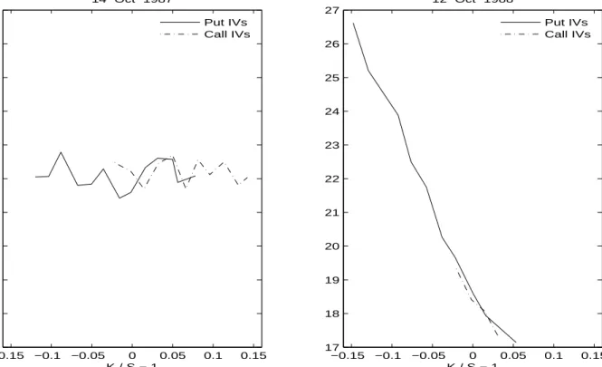
Rubinstein [233] and Bates [55], among others, note that prior to the 1987 market crash the Black and Scholes [63] (BS) formula priced option contracts quite accurately whereas after the crash it has been systematically underpricing out-of-the-money equity-index put contracts. This feature is evident from Figure 1, which is constructed from options on the S&P 500 futures. It shows the implied volatility function for near-maturity contracts traded both before and after October 19, 1987 (‘Black Monday’). The mild u-shaped pattern prevailing in the pre-crash implied volatilities is labeled a ‘volatility smile,’ in contrast to the asymmetric post-1987 ‘volatility smirk.’ Importantly, while the steepness and level of the implied volatility curve fluctuate day to day depending on market conditions, the curve has been asymmetric and upward sloping ever since 1987, so the smirk remains in place to the current date, e.g., Benzoni et al. [60]. In contrast, before the crash the implied volatility curve was invariably flat or mildly u-shaped as documented in, e.g., Bates [57]. Finally, we note that the post-1987 asymmetric smirk for index options contrasts sharply with the pattern for individual equity options, which possess flat or mildly u-shaped implied volatility curves (e.g., Bakshi et al. [37] and Bollen and Whaley [65]). Given the failures of the BS formula, much research has gone into relaxing the underlying assump-tions. A natural starting point is to allow volatility to evolve randomly, inspiring numerous studies that examine the option pricing implications of SV models. The list of early contributions includes Hull and White [174], Johnson and Shanno [187], Melino and Turnbull [211], Scott [238], Stein [244], Stein and Stein [245], and Wiggins [256]. Here we focus in particular on the Hull and White [174] model,

dp(t) = µ_pdt+pV(t)dWp(t) (33)

dV(t)

V(t) = µV dt+σV dWV(t), (34) where Wp and WV are standard Brownian motions. In general, shocks to returns and volatility may be (negatively) correlated, however for tractability Hull and White assume ρ= corr(dWp, dWV) = 0.

−0.15 −0.1 −0.05 0 0.05 0.1 0.15 17 18 19 20 21 22 23 24 25 26 27 K / S − 1

Black−Scholes IV (percent per year)

14−Oct−1987 Put IVs Call IVs −0.15 −0.1 −0.05 0 0.05 0.1 0.15 17 18 19 20 21 22 23 24 25 26 27 K / S − 1 12−Oct−1988 Put IVs Call IVs

Figure 1: Pre- and Post-1987 Crash Implied Volatilities. The plots depict Black-Scholes implied volatilities computed from near-maturity options on the S&P500 futures on October 14, 1986 (the week before the 1987 market crash) and a year later.

Under this assumption they show that, in a risk-neutral world, the premiumCHW on a European call option is the Black and Scholes price CBS _{evaluated at the average integrated varianceV,}

V = 1

T−t

Z _T

t

V(s)ds , (35)

integrated over the distributionh(V|V(t)) of V:

CHW(p(t), V(t) ) =

Z

CBS(V)h(V|V(t))dV . (36) The early efforts to identify a more realistic probabilistic model for the underlying return were slowed by the analytical and computational complexity of the option pricing problem. Unlike the BS setting, the early SV specifications do not admit closed-form solutions. Thus, the evaluation of the option price requires time-consuming computations through, e.g., simulation methods or numerical solution of the pricing partial differential equation by finite difference methods. Further, the presence of a latent factor, volatility, and the lack of closed-form expressions for the likelihood function complicate the estimation problem.

Consequently, much effort has gone into developing restrictions for the distribution of the under-lying return process that allow for (semi) closed-form solutions and are consistent with the empirical properties of the data. The ‘affine’ class of continuous-time models has proven particularly useful

in providing a flexible, yet analytically tractable, setting. Roughly speaking, the defining feature of affine jump-diffusions is that the drift term, the conditional covariance term, and the jump intensity are all a linear-plus-constant (affine) function of the state vector. The Vasicek [255] bond valuation model and the Cox et al. [112] intertemporal asset pricing model provide powerful examples of the advantages of the affine paradigm.

To illustrate the progress in option pricing applications built on affine models, consider the return dynamics

dp(t) = µ dt+pV(t)dWp(t) +ξp(t)dq(t) (37)

dV(t) = κ(V −V(t))dt+σV

p

V(t)dWV(t) +ξV(t)dq(t), (38) where Wp and WV are standard Brownian motions with non-zero correlation ρ = corr(dWp, dWV), q is a Poisson process, uncorrelated with Wp and WV, with jump intensity

λ(t) =λ0+λ1V(t), (39)

that is, Prob(dqt= 1) = λ(t)dt. The jump amplitudes variables ξp and ξV have distributions

ξ_V(t) ; exp(ξ_V) (40)

ξ_p(t)|ξ_V(t) ; N(ξ_p+ρ_ξξ_V(t), σ2_p). (41) Here volatility is not only stochastic but also subject to jumps which occur simultaneously with jumps in the underlying return process. The Black and Scholes model is a special case of (37)-(41) for constant volatility,V(t) =σ2_{,0≤t≤T, and no jumps,λ(t) = 0,0≤t≤T. The Merton [214] model}

arises from (37)-(41) if volatility is constant but we allow for jumps in returns.

More recently, Heston [170] has considered a special case of (37)-(41) with stochastic volatility but without jumps. Using transform methods he derives a European option pricing formula which may be evaluated readily through simple numerical integration. His SV model has GARCH-type features, in that the variance is persistent and mean reverts at a rateκto the long-run meanV. Compared to Hull and White’s [174] setting, Heston’s model allows for shocks to returns and volatility to be negatively correlated, i.e., ρ < 0, which creates a leverage-type effect and skews the return distribution. This feature is consistent with the properties of equity index returns. Further, a fatter left tail in the return distribution results in a higher cost for crash insurance and therefore makes out-of-the-money put options more expensive. This is qualitatively consistent with the patterns in implied volatilities observed after the 1987 market crash and discussed above.

Bates [56] has subsequently extended Heston’s approach to allow for jumps in returns and using similar transform methods he has obtained a semi-closed form solution for the option price. The addition of jumps provides a more realistic description of equity returns and has important option pricing implications. With diffusive shocks (e.g., stochastic volatility) alone a large drop in the value of the underlying asset over a short time span is very unlikely whereas a market crash is always possible as long as large negative jumps can occur. This feature increases the value of a short-dated put option, which offers downside protection to a long position in the underlying asset.

Finally, Duffie et al. [130] have introduced a general model with jumps to volatility which embeds the dynamics (37)-(41). In model (37)-(41), the likelihood of a jump to occur increases when volatility

is high (λ₁>0) and a jump in returns is accompanied by an outburst of volatility. This is consistent with what is typically observed during times of market stress. As in the Heston case, variance is persistent with a mean reversion coefficient κ towards itsdiffusive long-run mean V, while the total long-run variance mean is the sum of the diffusive and jump components. In the special case of constant jump intensity, i.e.,λ1 = 0, the total long-run mean isV+ξVλ0/κ. The jump term (ξV(t)dq(t)) fattens the right tail of the variance distribution, which induces leptokurtosis in the return distribution. Two effects generate asymmetrically distributed returns. The first channel is the diffusive leverage effect, i.e., ρ < 0, the second is the correlation between the volatility and the jump amplitude of returns generated through the coefficient ρ_ξ. Taken together, these effects increase model-implied option prices and help produce a realistic volatility smirk.

Several empirical studies rely on models of the form (37)-(41) in option-pricing applications. For instance, Bates [56] uses Deutsche Mark options to estimate a model with stochastic volatility and constant-intensity jumps to returns, while Bates [57] fits a jump-diffusion model with two SV factors to options on S&P 500 futures. In the latter case, the two SV factors combine to help capture features of the long-run memory in volatility while retaining the analytical tractability of the affine setting (see, e.g., Christoffersen et al. [101] for another model with similar features). Alternative approaches to model long memory in continuous-time SV models rely on the fractional Brownian motion process, e.g., Comte and Renault [108] and Comte et al. [107], while Breidt et al. [76], Harvey [166] and Deo et al. [118] consider discrete-time SV models (see Hurvich et al. [175] for a review). Bakshi et al. [34, 37] estimate a model similar to the one introduced by Bates [56] using S&P 500 options.

Other scholars rely on underlying asset return data alone for estimation. For instance, Andersen et al. [15] and Chernov et al. [95] use equity-index returns to estimate jump-diffusion SV models within and outside the affine (37)-(41) class. Eraker et al. [142] extend this analysis and fit a model that includes constant-intensity jumps to returns and volatility.

Finally, another stream of work examines the empirical implications of SV jump-diffusions using a joint sample of S&P 500 options and index returns. For example, Benzoni [59], Chernov and Ghysels [93], and Jones [189] estimate different flavors of the SV model without jumps. Pan [220] fits a model that has jumps in returns with time-varying intensity, while Eraker [141] extends Pan’s work by adding jumps in volatility.

Overall, this literature has established that the SV jump-diffusion model dramatically improves the fit of underlying index returns and options prices compared to the Black and Scholes model. Stochastic volatility alone has a first-order effect and jumps further enhance model performance by generating fatter tails in the return distribution and reducing the pricing error for short-dated options. The benefits of the SV setting are also significant in hedging applications.

Another aspect related to the specification of SV models concerns the pricing of volatility and jump risks. Stochastic volatility and jumps are sources of uncertainty. It is an empirical issue to determine whether investors demand to be compensated for bearing such risks and, if so, what the magnitude of the risk premium is. To examine this issue it is useful to write model (37)-(41) in so-called risk-neutral form. It is common to assume that the volatility risk premium is proportional to the instantaneous variance,η(t) =η_VV(t). Further, the adjustment for jump risk is accomplished by assuming that the amplitude ˜ξ_p(t) of jumps to returns has mean ˜ξ_p = ξ_p+η_p. These specifications are consistent with an arbitrage-free economy. More general specifications can also be supported in a

general equilibrium setting, e.g., a risk adjustment may apply to the jump intensityλ(t). However, the coefficients associated to these risk adjustments are difficult to estimate and to facilitate identification they typically are fixed at zero. Incorporating such risk premia in model (37)-(41) yields the following risk-neutral return dynamics (e.g., Pan [220] and Eraker [141]):

dp(t) = (r−µ∗)dt+pV(t)dWfp(t) + ˜ξp(t)dq(t) (42)

dV(t) = [κ(V −V(t)) +η_V V(t) ]dt+σV

p

V(t)dWfV(t) +ξV(t)dq(t), (43)

whereris the risk-free rate,µ∗_{a jump compensator term,W}f_pandf_{WV are standard Brownian motions}

under this so-calledQmeasure, and the risk-adjusted jump amplitude variable ˜ξ_pis assumed to follow the distribution,

˜

ξ_p(t)|ξ_V(t);N(˜ξ_p+ρ_ξξ_V(t), σ2_p). (44) Several studies estimate the risk-adjustment coefficients η_V and η_p for different specifications of model (37)-(44); see, e.g., Benzoni [59], Broadie et al. [78], Chernov and Ghysels [93], Eraker [141], Jones [189], and Pan [220]. It is found that investors demand compensation for volatility and jump risks and these risk premia are important for the pricing of index options. This evidence is reinforced by other studies examining the pricing of volatility risk using less structured but equally compelling procedures. For instance, Coval and Shumway [111] find that the returns on zero-beta index option straddles (i.e., combinations of calls and puts that have offsetting covariances with the index) are significantly lower than the risk-free return. This evidence suggests that in addition to market risk at least a second factor (likely, volatility) is priced in the index option market. Similar conclusions are obtained by Bakshi and Kapadia [36], Buraschi and Jackwerth [79], and Broadie et al. [78].

V.2. Risk-Free Bonds and their Derivatives

The market for (essentially) risk-free Treasury bonds is liquid across a wide maturity spectrum. It turns out that no-arbitrage restrictions constrain the allowable dynamics in the cross-section of bond yields. Much work has gone into the development of tractable dynamic term structure models capable of capturing the salient time-series properties of interest rates while respecting such cross-sectional no-arbitrage conditions. The class of so-called ‘affine’ dynamic term structure models provides a flexible and arbitrage-free, yet analytically tractable, setting for capturing the dynamics of the term structure of interest rates. Following Duffie and Kan [129], Dai and Singleton [114, 115], and Piazzesi [227], the short term interest rate, y0(t), is an affine (i.e., linear-plus-constant) function of a vector of state

variables, X(t) ={xi(t), i= 1, . . . , N}: y0(t) =δ0+ N X i=1 δixi(t) =δ0+δ0XX(t), (45)

where the state-vector X has risk-neutral dynamics

dX(t) = ˜K( ˜Θ−X(t))dt+ ΣpS(t)dfW(t). (46)

In equation (46), Wf is anN-dimensional Brownian motion under the so-calledQ-measure, ˜K and ˜Θ are N×N matrices, andS(t) is a diagonal matrix with the ith diagonal element given by [S(t)]ii=

α_i+β0

iX(t). Within this setting, the time-t price of a zero-coupon bond with time-to-maturity τ is given by

P(t, τ) =eA(τ)−B(τ)0X(t), (47) where the functionsA(τ) andB(τ) solve a system of ordinary differential equations (ODEs); see, e.g., Duffie and Kan [129]. Semi-closed form solutions are also available for bond derivatives, e.g., bond options as well as caps and floors (e.g., Duffie et al. [130]).

In empirical applications it is important to also establish the evolution of the state vectorX under the physical probability measureP, which is linked to theQ-dynamics (46) through a market price of risk, Λ(t). Following Dai and Singleton [114] the market price of risk is often given by

Λ(t) =pS(t)λ , (48)

where λis an N ×1 vector of constants. More recently, Duffee [127] proposed a broader ‘essentially affine’ class, which retains the tractability of standard models but, in contrast to the specification in equation (48), allows compensation for interest rate risk to vary independently of interest rate volatility. This additional flexibility proves useful in forecasting future yields. Subsequent generalization are in Duarte [124] and Cheridito et al. [92].

Litterman and Scheinkman [201] demonstrate that virtually all variation in U.S. Treasury rates is captured by three factors, interpreted as changes in ‘level,’ ‘steepness,’ and ‘curvature.’ Consistent with this evidence, much of the term-structure literature has focused on three-factor models. One problem with these models, however, is that the factors are latent variables void of immediate eco-nomic interpretation. As such, it is challenging to impose appropriate identifying conditions for the model coefficients and in particular to find the ideal representation for the ‘most flexible’ model, i.e., the model with the highest number of identifiable coefficients. Dai and Singleton [114] conduct an ex-tensive specification analysis of multi-factor affine term structure models. They classify these models into subfamilies according to the number of (independent linear combination of) state variables that determine the conditional variance matrix of the state vector. Within each subfamily, they proceed to identify the models that lead to well-defined bond prices (a condition they label ‘admissibility’) and among the admissible specifications they identify a ‘maximal’ model that nests econometrically all others in the subfamily. Joslin [190] builds on Dai and Singleton’s [114] work by pursuing identifi-cation through a normalization of the drift term in the state vector dynamics (instead of the diffusion term, as in Dai and Singleton [114]). Duffie and Kan [129] follow an alternative approach to obtain an identifiable model by rotating from a set of latent state variables to a set of observable zero-coupon yields. Collin-Dufresne et al. [104] build on the insights of both Dai and Singleton [114] and Duffie and Kan [129]. They perform a rotation of the state vector into a vector that contains the first few components in the Taylor series expansion of the yield curve around a maturity of zero and their quadratic variation. One advantage is that the elements of the rotated state vector have an intuitive and unique economic interpretation (such as level, slope, and curvature of the yield curve) and there-fore the model coefficients in this representation are identifiable. Further, it is easy to construct a model-independent proxy for the rotated state vector, which facilitates model estimation as well as interpretation of the estimated coefficients across models and sample periods.

This discussion underscores an important feature of affine term structure models. The dependence of the conditional factor variance S(t) on one or more of the elements in X introduces stochastic

volatility in the yields. However, when a square-root factor is present parametric restrictions (admis-sibility conditions) need to be imposed so that the conditional varianceS(t) is positive over the range of X. These restrictions affect the correlations among the factors which, in turn, tend to worsen the cross-sectional fit of the model. Specifically, CIR models in whichS(t) depends on all the elements of

X require the conditional correlation among the factors to be zero, while the admissibility conditions imposed on the matrixK renders the unconditional correlations non-negative. These restrictions are not supported by the data. In contrast, constant-volatility Gaussian models with no square-root fac-tors do not restrict the signs and magnitude of the conditional and unconditional correlations among the factors but they do, of course, not accommodate the pronounced and persistent volatility fluctua-tions observed in bond yields. The class of models introduced by Dai and Singleton [114] falls between these two extremes. By including both Gaussian and square-root factors they allow for time-varying conditional volatilities of the state variables and yet they do not constrain the signs of some of their correlations. This flexibility helps to address the trade off between generating realistic correlations among the factors while capturing the time-series properties of the yields’ volatility.

A related aspect of (unconstrained) affine models concerns the dual role that square-root fac-tors play in driving the time-series properties of yields’ volatility and the term structure of yields. Specifically, the time-t yieldy_τ(t) on a zero-coupon bond with time-to-maturity τ is given by

P(t, τ) =e−τ yτ(t)_{. (49)} Thus, we have y_τ(t) =−A(τ) τ + B(τ)0 τ X(t). (50)

It is typically assumed that the B matrix has full rank and therefore equation (50) provides a direct link between the state-vectorX(t) and the term-structure of bond yields. Further, Itˆo’s Lemma implies that the yieldyτ also follows a diffusion process:

dyτ(t) =µyτ(X(t), t)dt+

B(τ)0

τ Σ

p

S(t)dfW(t). (51)

Consequently, the (instantaneous) quadratic variation of the yield given as the squared yield volatility coefficient for y_τ is Vyτ(t) = B(τ)0 τ ΣS(t) Σ 0 B(τ) τ . (52)

The elements of theS(t) matrix are affine in the state vectorX(t), i.e., [S(t)]_ii=α_i+β0_iX(t). Further, invoking the full rank condition onB(τ), equation (50) implies that each state variable in the vector

X(t) is an affine function of the bond yieldsY(t) ={yτj(t), j= 1, . . . , J}. Thus, for anyτ there is a

set of constants a_{τ , j},j= 0, . . . , J, so that

V_yτ(t) =a_{τ ,0}+ J

X

j=1

a_{τ , j}y_τj(t). (53)

Hence, the current quadratic yield variation for bonds at any maturity is a linear combination of the term structure of yields. As such, the market is complete, i.e., volatility is perfectly spanned by a portfolio of bonds.

Collin-Dufresne and Goldstein [103] note that this spanning condition is unnecessarily restrictive and propose conditions which ensures that volatility no longer directly enters the main bond pricing equation (47). This restriction, which they term ‘unspanned stochastic volatility’ (USV), effectively breaks the link between the yields’ quadratic variation and the level of the term structure by imposing a reduced rank condition on the B(τ) matrix. Further, since their model is a special (nested) case of the affine class it retains the analytical tractability of the affine model class. Recently Joslin [190] has derived more general conditions for affine term structure models to exhibit USV. His restrictions also produce a market incompleteness (i.e., volatility cannot be hedged using a portfolio of bonds) but do not constrain the degree of mean reversion of the other state variables so that his specification allows for more flexibility in capturing the persistence in interest rate series. (See also the USV conditions in the work by Trolle and Schwartz [253]).

There is conflicting evidence on the volatility spanning condition in fixed income markets. Collin-Dufresne and Goldstein (2002) find that swap rates have limited explanatory power for returns on at-the-money ‘straddles,’ i.e., portfolios mainly exposed to volatility risk. Similar findings are in Heidari and Wu [169], who show that the common factors in LIBOR and swap rates explain only a limited part of the variation in the swaption implied volatilities. Moreover, Li and Zhao [197] conclude that some of the most sophisticated multi-factor dynamic term structure models have serious difficulties in hedging caps and cap straddles, even though they capture bond yields well. In contrast, Fan et al. [143] argue that swaptions and even swaption straddles can be well hedged with LIBOR bonds alone, supporting the notion that bond markets are complete.

More recently other studies have examined several versions of the USV restriction, again coming to different conclusions. A direct comparison of these results, however, is complicated by differences in the model specification, the estimation method, and the data and sample period used in the estimation. Collin-Dufresne et al. [105] consider swap rates data and fit the model using a Bayesian Markov Chain Monte Carlo method. They find that a standard three-factor model generates a time series for the variance state variable that is essentially unrelated to GARCH estimates of the quadratic variation of the spot rate process or to implied variances from options, while a four-factor USV model generates both realistic volatility estimates and a good cross-sectional fit. In contrast, Jacobs and Karoui [177] consider a longer data set of U.S. Treasury yields and pursue quasi-maximum likelihood estimation. They find the correlation between model-implied and GARCH volatility estimates to be high. However, when estimating the model with a shorter sample of swap rates, they find such correlations to be small or negative. Thompson [250] explicitly tests the Collin-Dufresne and Goldstein [103] USV restriction and rejects it using swap rates data. Bikbov and Chernov [62], Han [164], Jarrow et al. [182], Joslin [191], and Trolle and Schwartz [254] rely on data sets of derivatives prices and underlying interest rates to better identify the volatility dynamics.

Andersen and Benzoni [12] directly relate model-free realized volatility measures (constructed from high-frequency U.S. Treasury data) to the cross-section of contemporaneous bond yields. They find that the explanatory power of such regressions is very limited, which indicates that volatility is not spanned by a portfolio of bonds. The evidence in Andersen and Benzoni [12] is consistent with the USV models of Collin-Dufresne et al. [105] and Joslin [190], as well as with a model that embeds weak dependence between the yields and volatility as in Joslin [191]. Moreover, Duarte [125] argues that the effects of mortgage-backed security hedging activity affects both the interest rate volatility implied by

options and the actual interest rate volatility. This evidence suggests that variables that are not in the span of the term structure of yields and forward rates contribute to explain volatility in fixed income markets. Also related, Wright and Zhou [258] find that adding a measure of market jump volatility risk to a regression of excess bond returns on the term structure of forward rates nearly doubles the R2 _{of the regression. Taken together, these findings suggest more generally that genuine SV models}

are critical for appropriately capturing the dynamic evolution of the term structure.

VI. Estimation Methods

There are a very large number of alternative approaches to estimation and inference for parametric SV models and we abstain from a thorough review. Instead, we point to the basic challenges that exist for different types of specifications, how some of these were addressed in the early literature and finally provide examples of methods that have been used extensively in recent years. Our exposition continues to focus on applications to equity returns, interest rates, and associated derivatives.

Many of the original SV models were cast in discrete time, inspired by the popular GARCH paradigm. In that case, the distinct challenge for SV models is the presence of a strongly persistent latent state variable. However, more theoretically oriented models, focusing on derivatives applica-tions, were often formulated in continuous time. Hence, it is natural that the econometrically-oriented literature has moved in this direction in recent years as well. This development provides an added complication as the continuous-time parameters must be estimated from discrete return data and without direct observations on volatility. For illustration, consider a fully parametric continuous-time SV model for the asset return r with conditional variance V and coefficient vector Ψ. Most methods to estimate Ψ rely on the conditional densityf for the data generating process,

f(r(t), V(t)| I(t−1),Ψ) =f_r|V(r(t)|V(t),I(t−1),Ψ)×fV(V(t)| I(t−1),Ψ), (54) where I(t−1) is the available information set at time t−1. The main complications are readily identified. First, analytic expressions for the discrete-time transition (conditional) density, f, or the discrete-time moments implied by the data generating process operating in continuous time, are often unavailable. Second, volatility is latent in SV models, so that even if a closed-form expression forf is known, direct evaluation of the above expression is infeasible due to the absence of explicit volatility measures. The marginal likelihood with respect to the observable return process alone is obtained by integrating over all possible paths for the volatility process, but this integral has a dimension corresponding to sample size, rendering the approach infeasible in general.

Similar issues are present when estimating continuous-time dynamic term structure models. Fol-lowing Piazzesi [228], a change of variable gives the conditional density for a zero-coupon yieldyon a bond with time to maturityτ:

f(y_τ(t)| I(t−1),Ψ) =f_X(g(y_τ(t),Ψ)| I(t−1),Ψ)× | 5_yg(y_τ(t),Ψ)|. (55) Here the latent state vector X has conditional density f_X, the function g(·,Ψ) maps the observable yield y intoX,X(t) =g(yτ(t),Ψ), and 5yg(yτ(t),Ψ) is the Jacobian determinant of the transforma-tion. Unfortunately, analytic expressions for the conditional densityfX are known only in some special

cases. Further, the mapping X(t) =g(y_τ(t),Ψ) holds only if the model provides an exact fit to the yields, while in practice different sources of error (e.g., model mis-specification, microstructure effects, measurement errors) inject a considerable degree of noise into this otherwise deterministic linkage (for correct model specification) between the state vector and the yields. As such, a good measure of X

might not be available to evaluate the conditional density (55).

VI.1. Estimation via Discrete-Time Model Specification or Approximation

The first empirical studies have estimated discrete-time SV models via a (Generalized) Method of Moments procedure by matching a number of theoretical and sample moments, e.g., Chan et al. [89], Ho et al. [171], Longstaff and Schwartz [204], and Melino and Turnbull [211]. These models were either explicitly cast in discrete time or were seen as approximate versions of the continuous-time process of interest. Similarly, several authors estimate diffusive affine dynamic term structure models by approximating the continuous-time dynamics with a discrete-time process. If the error terms are stipulated to be normally distributed, the transition density of the discretized process is multivariate normal and computation of unconditional moments then only requires knowledge of the first two moments of the state vector. This result facilitates quasi-maximum likelihood estimation. In evaluating the likelihood function, some studies suggest using closed-form expressions for the first two moments of the continuous-time process instead of the moments of the discretized process (e.g., Fisher and Gilles [145] and Duffee [127]), thus avoiding the associated discretization bias. This approach typically requires some knowledge of the state of the system which may be obtained, imperfectly, through matching the system, given the estimated parameter vector, to a set of observed zero-coupon yields to infer the state vector X. A modern alternative is to use the so-called particle filter as an efficient filtering procedure for the unobserved state variables given the estimated parameter vector. We provide more detailed accounts of both of these procedures later in this section.

Finally, a number of authors develop a simulated maximum likelihood method that exploit the specific structure of the discrete-time SV model. Early examples are Danielsson and Richard [117] and Danielsson [116] who exploit the Accelerated Gaussian Importance Sampler for efficient Monte Carlo evaluation of the likelihood. Subsequent improvements were provided by Fridman and Harris [149] and Liesenfeld and Richard [200], with the latter relying on Efficient Importance Sampling (EIS). In a second step, EIS can also be used for filtering the latent volatility state vector. In general, these inference techniques provide quite impressive efficiency but the methodology is not always easy to generalize beyond the structure of the basic discrete-time SV asset return model. We discuss the general inference problem for continuous-time SV models for which the lack of a closed-form expression for the transition density is an additional complicating factor in a later section.

VI.2. Filtering the Latent State Variable Directly During Estimation

Some early studies focused on direct ways to extract estimates of the latent volatility state variable in discrete-time SV asset return models. The initial approach was based on quasi-maximum likelihood (QML) methods exploiting the Kalman filter. This method requires a transformation of the SV model to a linear state-space form. For instance, Harvey and Shephard [168] consider a version of the Taylor’s