Macroeconomic Implications of Fiscal Policy in a Small Open Economy

(1)

Persistent link:

http://hdl.handle.net/2345/bc-ir:108102

This work is posted on

eScholarship@BC

,

Boston College University Libraries.

Boston College Electronic Thesis or Dissertation, 2018

Copyright is held by the author. This work is licensed under a Creative Commons Attribution 4.0 International License (http://creativecommons.org/licenses/by/4.0).

Macroeconomic Implications of Fiscal

Policy in a Small Open Economy

(2)

MACROECONOMIC

IMPLICATIONS OF FISCAL

POLICY IN A SMALL OPEN

ECONOMY

Krastina Dzhambova-Andonova

A dissertation

submitted to the Faculty of the department of Economics

in partial fulfillment

of the requirements for the degree of Doctor of Philosophy

Boston College

Morrissey College of Arts and Sciences Graduate School

(3)

(4)

MACROECONOMIC IMPLICATIONS OF FISCAL POLICY IN A SMALL OPEN ECONOMY

Krastina Dzhambova-Andonova Advisor: Professor Peter N. Ireland

This dissertation deals with the macroeconomic implications of fiscal policy in small open economies with a particular emphasis on emerging economies. I use both

em-pirical and theoretical approaches to distinguish key di↵erence in the design of fiscal

policy between emerging and developed economies. I also analyze the macroeconomic

consequences of di↵erences in the conduct of fiscal policy. Thus, the dissertation is

focused on the interplay between fiscal policy and business cycle dynamics. Recent policy challenges in developed economies, such as monetary authorities grappling with the zero lower bound on short run nominal rates and fiscal stimulus packages emerging as an important policy tool, have sparked renewed academic interest in the topic of fiscal policy and business cycles. Institutional and macroeconomic features in emerging economies make the macroeconomic aspects of fiscal policy an important research agenda and one to which this dissertation contributes.

A number of papers have documented fiscal policy pro cyclicality in terms of stronger co-movement between government expenditure and macroeconomic fundamentals in emerging and developing economies. This feature of the data raises a 2 important questions: 1) does fiscal policy reinforce the macroeconomic cycle in these countries leading to a heighten macroeconomic volatility (“when it rains, it pours”), and 2) is the fiscal stance in these economies due to unique macroeconomic features or is it the consequence of institutional and political imperfections? The first chapter,

titled “When it rains, it pours”: fiscal policy, credit constraints and business cycles

in emerging and developed economies, sets out to answer these questions by compar-atively studying a group of developed and emerging economies. I estimate a panel

(5)

structural vector autoregressive model to investigate if government consumption ex-penditure responds more pro cyclically to fundamentals and what role international financial conditions play for the fiscal stance and for the volatility of the cycle in emerging economies relative to developed. My findings suggest the response to

out-put fluctuations is not systematically di↵erent in emerging governments relative to

developed economies’. However, emerging governments curtail spending in response to increases in the sovereign borrowing rate which forces their consumption expendi-ture to act more pro cyclically. I find evidence of higher fiscal discretion in emerging

economies. However, the efficacy of government consumption expenditure is

substan-tially lower in emerging economies than in developed. Thus fiscal policy ends up being responsible for a lower share of business cycle volatility in emerging economies than in developed.

In the second chapter, titled Estimating the Dynamics of Fiscal Financing in

Emerg-ing Economies, I propose a strategy for estimating the government financing rule for an emerging economy. The estimation uses the structural VAR impulse responses ob-tained in the previous chapter to discipline the parameters of a small open economy real business cycle model with a public sector. The parameters can be split into two

groups: those influencing the e↵ectiveness of fiscal policy (i.e the multiplier MG

Y ) and

the parameters governing the financing of the exogenous stream of government con-sumption. The empirical response to interest rate shocks puts restrictions on the first group of parameters governing the size of the multiplier. The empirical response to a government consumption shock can be used to obtain estimates of the fiscal policy rule. I construct a model with a role for both interest rate shocks and government consumption shocks. A natural estimation approach in this case is impulse response matching.

(6)

List of Figures

1.1 Contemporaneous correlation between government expenditure and

real GDP . . . 40

1.2 Volatility of government expenditure and real GDP. . . 41

1.3 Government expenditure cyclicality and country size . . . 42

1.4 Government expenditure cyclicality in terms of amplitude . . . 42

1.5 Elasticity of government expenditure and revenue with respect to real output . . . 43

1.6 Contemporaneous correlation between government consumption and real GDP . . . 44

1.7 Volatility of government consumption and real GDP . . . 45

1.8 Contemporaneous correlation between the cyclical component of GDP and government expenditure by group . . . 46

1.9 Contemporaneous correlation between the cyclical component of GDP and net government expenditure by group . . . 47

1.10 Government size across groups . . . 48

1.11 Distribution of the yield-to-maturity for the EMBI+ and the GBI index 49 1.12 Median yield for the countries in the sample . . . 50

1.13 Realized yield for the countries in the sample . . . 52

1.14 Yields for the distressed European economies . . . 53

(9)

1.16 Estimates of the e↵ect of the first lag of the designated variable on the

safe rate . . . 55

1.17 Shock to government consumption . . . 56

1.18 Government Consumption Multiplier . . . 57

1.19 Shock to output . . . 58

1.20 Multiplier e↵ect of an output shock . . . 59

1.21 Shock to the country’s sovereign rate . . . 60

1.22 Multiplier e↵ect of a sovereign rate shock . . . 61

1.23 Shock to the safe rate . . . 62

1.24 Government shock volatility by country . . . 63

1.25 Output shock volatility by country . . . 64

1.26 Sovereign rate shock volatility by country . . . 65

1.27 Government shock volatility by country (coefficient of variation) . . . 66

1.28 Output shock volatility by country (coefficient of variation) . . . 67

1.29 Sovereign rate shock volatility by country (coefficient of variation) . . 68

1.30 AIC for GMM and fixed e↵ects . . . 68

1.31 Estimates of Ai=0,1 (developed economies) . . . 70

1.32 Estimates of Ai=0,1 (emerging economies) . . . 71

1.33 Government Response Function: Dynamic panel data estimation . . . 72

1.34 Government Response Function: Robustness Check 1 . . . 73

1.37 Variance decomposition: government consumption shocks . . . 76

1.38 Variance decomposition: output shocks . . . 76

1.39 Variance decomposition: sovereign rate shocks . . . 77

1.40 Government consumption shock; FE estimates . . . 78

(10)

1.42 Sovereign rate shock; FE estimates . . . 80

1.43 Eigenvalues of selected matrices . . . 81

1.44 Autoregressive coefficient of the government rate; estimates by country 82 2.1 Schematic representation of the estimation approach in Uribe and Yue (2006) . . . 103

2.2 Schematic representation of proposed estimation strategy: the lump sum taxation case . . . 103

2.3 Schematic representation of proposed estimation strategy: distortionary taxation . . . 104

2.4 Schematic representation of the labor market in a closed economy model . . . 105

2.5 Parameterization and implied parameter values in the closed economy stylized model . . . 105

2.6 Impulse response to a government consumption shock in the closed economy . . . 106

2.7 Impulse response to a government consumption shock in the closed economy . . . 106

2.8 Government consumption shock: closed versus open economy . . . . 107

2.9 Introducing a working capital constraint . . . 108

2.10 Sensitivity to ⌘ . . . 109

2.11 Sensitivity to the capital adjustment cost . . . 110

2.12 Sensitivity to habit formation µ . . . 111

(11)

List of Tables

(12)

Acknowledgements

I am extremely grateful to my advisors: Professor Peter Ireland, Professor Christo-pher Baum and Professor Fabio Ghironi for their invaluable guidance, encouragement, patience and support. I owe them a debt of gratitude for their kindness and expertise.

I am grateful to Professor Tracy Regan, Professor Can Erbil and Professor Richard Tresch for mentoring me as an educator.

I am thankful for the support and advice of my brilliant economist friends: Dr. Ana Lariau, Dr. Solvejg Wewel, Marco Brianti, Dr. Zulma Barrail Halley, Dr. Zhaochen He, Dr. Jinghan Cai, Dr. Frank Georges and Dr. Naijing Huang. I also thank Dr. Eyal Dvir for his friendship and encouragement.

I am indebted to my supervisors at the Boston College Research Services Center- Rani Dalgin, Barry Schaudt and Constantin Andronache for being extremely supportive and encouraging in my dissertation writing process.

(13)

Chapter 1

“When it rains, it pours”: fiscal

policy, credit constraints and

business cycles in emerging and

developed economies

1.1

Introduction

The empirical international finance literature has long emphasized excess volatility that business cycles in emerging and poor economies exhibit. Relative to the devel-oped world, these economies have higher volatility of all aggregate demand compo-nents as well as more frequent and deeper crises (Uribe and Schmitt-Grohe (2017)). Another strand of research sheds light on the tendency of fiscal policy to be pro-cyclical in these economies. This paper explores the relationship between these two stylized facts. In particular, I study the question of business cycle volatility in emerg-ing economies through the lens of the “when it rains, it pours” phenomenon. Dubbed so by Kaminsky et al. (2004), this is a situation in which recessions are reinforced by

(14)

capital outflows coupled with a pro-cyclical policy stance.1 _{Kaminsky et al. (2004)}

among others2 _{document that while in general net capital flows are pro-cyclical across}

poor, emerging and developed economies, the cyclicality of (fiscal) policy variables dif-fers between the developing and developed group. In particular, developing economies exhibit fiscal policy pro-cyclicality which is difficult to justify as a policy prescription.3

This paper aims to uncover the reasons for and the consequences of fiscal pro-cyclicality. On one hand, policymakers themselves could be the source of volatility through discretionary interventions. On the other hand, it is reasonable to expect that policymakers in the developing and emerging world face constraints which impede their role as insurers against macroeconomic volatility. International borrowing costs have been emphasized as important drivers of business cycle fluctuations in emerging economies. Finally, even if policy itself does not cause or contribute to

macroeco-nomic volatility, the same policy design will lead to di↵erent outcomes both in terms

of policy and private sector variables when the underlying macro shocks are di↵erent.

In short we want to ask whether the macroeconomic woes of these economies are self-induced or the result of more volatile underlying shocks, coupled with potentially tighter constraints faced by these governments. If the latter is true, we also want to know if the excess volatility originates at home through a more volatile process for

1_{Kaminsky et al. (2004) explore both fiscal and monetary policy cyclicality among developing,} emerging and developed countries. This paper focuses on fiscal policy although as a natural contin-uation the interaction between fiscal and monetary policy as well as exchange rate policy is to be considered.

2_{see Talvi and Vegh (2005), Gavin and Perotti (1997).}

3_{The term pro-cyclicality itself requires a careful definition. As emphasized by Kaminsky et al.} (2004), perhaps the most convenient measure to use to identify potential di↵erences in the conduct of fiscal policy is government expenditure as opposed to revenue and primary balance in levels and as a share of GDP. In terms of government expenditure, fiscal pro-cyclicality is defined as a positive co-movement between government expenditure and GDP. Other researchers have defined pro-cyclicality in terms of taxes: the government raises tax rates in recessions. Direct evidence on tax rates is sparse so researchers have used government revenue statistics and anecdotal evidence to make the case for fiscal pro-cyclicality in developing economies. Finally, primary balance statistics highlight that fiscal outcomes are di↵erent for the developing world but they are hard to use to disentangle the causes behind those results.

(15)

GDP, for example, or abroad through asset price shocks. In this context, I try to assess what fraction of business cycle fluctuations can be attributed to sovereign rate shocks versus policy shocks.

In order to understand the causes behind the “when it rains, it pours” phenomenon, I estimate a panel SVAR on a large group of developed and emerging economies. I focus on government consumption expenditure as the fiscal policy variable with the largest cross-country data availability. The analysis has to overcome the issues of en-dogeneity between 1) fiscal policy and fundamentals 2) international borrowing cost and fundamentals and 3) international borrowing cost and fiscal policy. A number of papers have emphasized the feedback between fundamentals and borrowing costs for

emerging economies.4 _{Fiscal policy variables also both respond to and influence the}

state of the economy. Finally, fluctuations in the price of externally traded sovereign debt put a constraint on policymakers’ ability to use fiscal policy for stabilization. There are several pass-through channels for a sovereign interest rate shock to influ-ence the cycle. First, if government spending contracts in response to increases in

the borrowing cost, there is a standard multiplier e↵ect which decreases output and

a↵ects investment and consumption contingent on wealth e↵ects and the strength of

Ricardian equivalence. Second, the government might shift part of the debt burden domestically thus crowding out investment and consumption. Finally, rising sovereign

rates can a↵ect the private economy if interest rate shocks pass through to

house-holds and firms via the banking sector.5 _{In order to shed light on these questions,}

the analysis needs to isolate orthogonal shocks to policy variables, fundamentals and international borrowing costs. Although fiscal pro-cyclicality is normally discussed in the context of emerging and developing economies, the European debt crisis made

4_{see Uribe and Yue (2006), Mendoza and Yue (2012).}

5_{see De Marco (forthcoming) for quantifying government debt distress pass-through to firm loans} in the context of developed economies and Arteta and Hale (2008) in the context of emerging economies.

(16)

the interaction between fiscal policy, government finances and the real economy a relevant issue for developed economies as well. In contrast to much of the literature, this paper studies both developed and emerging economies. I compare the behavior

and the e↵ect of government consumption spending across the two groups. I also

characterize the e↵ect of sovereign rate shocks on government consumption spending

as well as their direct and indirect e↵ect on private sector variables.

My identification strategy combines the Blanchard and Perotti (2002) SVAR approach to identify fiscal shocks and Uribe and Yue (2006) identification of external borrowing cost shocks. The methodology proposed by Blanchard and Perotti (2002) uses insti-tutional knowledge to put constraints on the impact matrix in a VAR analysis. In particular, the identification scheme assumes that discretionary fiscal responses take place with one period delay. The use of quarterly data is essential for implementing this identification strategy. For the purpose of identifying external borrowing costs, Uribe and Yue (2006) propose an ordering of the impact matrix which leads to im-pulse responses consistent with the standard small open economy real business cycle

model (SOE RBC). The current study o↵ers a unified framework for considering the

interactions among fundamentals, fiscal policy shocks and external financial

condi-tions.6_{Apart from the variables commonly included in the analysis, I also consider}

the interplay among the government response function, the dependence of spreads on both aggregate conditions and the government policy stance. This approach allows

6_{Another strategy for identifying the e}_↵_{ect of fiscal policy changes at business cycle frequency} is the narrative approach advocated by Romer and Romer (2010) among others. The narrative ap-proach uses information contained in government documents and announcements to identify periods of fiscal expansion or consolidation which are unrelated to the business cycle. The identification pro-cedure which uses military build up in wartime to identify government spending episodes unrelated to the business cycle is a special case of the narrative approach. Examples of this approach used on U.S data include Barro (1981), Hall (1986), Hall (2009), Rotemberg and Woodford (1992), Barro and Redlick (2011). As military build-up episodes are not common during the same time as most detailed macroeconomic data is available for the developing world, I adhere to the SVAR identification ap-proach to estimate the policy reaction function and the government spending multiplier.Sheremirov and Spirovska (2017) exploit a new military spending database to estimate multipliers for a large number of countries. Despite the di↵erence in identification, our estimates are in line.

(17)

me to retrieve estimates of the policy response function to output and international

borrowing costs as well as the coefficients on the government debt pricing function.

I also trace out the dynamic e↵ect of orthogonal shocks to income, sovereign yields

and government spending.

My findings suggest that government consumption, a category of government expen-diture, is pro-cyclical for both emerging and developed economies. The systematic response of both types of economies to output fluctuations is virtually the same. Emerging economies are however more sensitive for changes in international bor-rowing conditions. Higher output relaxes international borbor-rowing constraints. As a result, GDP shocks lead to an overall bigger increase in government consumption in emerging economies. This finding suggests that as far as government consumption is concerned, increases in this fiscal expenditure component during good times are not symptomatic of political frictions. Instead, the higher fiscal pro-cyclicality in emerg-ing economies is the result of these governments beemerg-ing more sensitive to international borrowing conditions. However, the analysis reveals that discretionary interventions are much more common in the emerging world. This raises concerns because a higher

degree of policy discretion has been shown to have a negative e↵ect on long run growth

and volatility.

I investigate the di↵erential role of international financial conditions for policy and

business cycle outcomes of emerging and developed economies along two dimensions: shocks to the international safe borrowing rate and shocks to the price of a country’s government debt on international markets. Fluctuations in the safe rate have a neg-ligible impact on the business cycle and the fiscal stance in either group of countries.

Shocks to the government borrowing rate have di↵erent implications for the developed

(18)

contrac-tionary in both economies. In the emerging group these shocks are more important for output fluctuations, while in the developed group they matter relatively more for investment dynamics.

My results also shed light on the efficacy of government consumption as a policy tool.

The estimated long run multiplier e↵ect of government consumption on output is less

than 1 for both country groups. However, the government consumption multiplier is twice as high for the developed group, pointing to a substantially impaired ability of government consumption shocks to influence the economy in emerging countries. My results also imply that government consumption expenditure shocks account for a smaller fraction of business cycle fluctuations in emerging economies. Despite the high volatility of these shocks in the emerging world, they claim a smaller share of the volatility of macroeconomic variables because of the smaller multiplier. Shocks to government consumption also account for a smaller share of the sovereign rate fluc-tuations emphasizing the fact that these governments have been more careful about international borrowing conditions. The paper provides estimates based on the of-ficially reported economic activity. Informality is currently outside the scope of the study.

In this paper I also document di↵erences in fiscal statistics and their relationship with

the cycle among a large group of poor, emerging and rich countries. I highlight that in terms of correlations to the cycle, government expenditure is pro-cyclical in poor and emerging economies as stressed in the literature. It is important however to look at individual components of government expenditure as this is a fairly large category which encompasses all of government expense as well as investment (Table 1.1). When focusing specifically on government consumption of goods and services, I find that

(19)

stemming from higher volatility of government consumption rather than cyclicality. The SVAR analysis currently focuses on government consumption expenditure. As

confirmed by summary statistics the distinction among di↵erent components of

gov-ernment expenditure is important. Govgov-ernment consumption expenditure is only one

component of automatic stabilization. Therefore, lack of other automatic

stabiliz-ers (e.g. social transfstabiliz-ers (unemployment benefits, safety-net program), retirement and health benefits, progressive taxes and proportional taxes) in emerging economies

might be behind the di↵erence in government expenditure cyclicality.7

Recent policy challenges in developed economies, such as monetary authorities grap-pling with the zero lower bound on short run nominal rates and fiscal stimulus pack-ages emerging as an important policy tool, have sparked renewed academic interest in the topic of fiscal policy and business cycles. In the next section I discuss how this paper relates to several branches of the literature: discretionary fiscal policy, po-litical frictions and macroeconomic outcomes, cost of borrowing and business cycles, external shocks and macroeconomic volatility. Section 1.3 describes the sources and construction of the dataset used in the paper. Section 1.4 describes the behavior of key fiscal variables across poor, emerging and developed economies. Section 1.5 discusses the SVAR methodology while section 1.6 discusses the empirical results. Section 1.7 and section 1.8 focus on the variance and the variance decomposition of estimated shocks. Section 1.9 presents robustness checks which extend the analysis to subsets of the data or employ an alternative estimation strategy. Section 1.10 concludes.

7_{McKay and Reis (2016) provide model-based estimates of the ability of US built-in stabilizers} to decrease consumption and output volatility. They find that the social insurance role (the tax-and-transfer system) of stabilizers is more important than the New Keynesian demand stabilization channel.

(20)

1.2

Links to the Literature

The vast majority of the studies on discretionary fiscal policy are conducted on US and to a lesser extent OECD data. Using US data and a VAR approach, Blanchard and Perotti (2002) estimate a government spending multiplier around 1; Fatas and Mihov (2001) obtain estimates well above 1 while Mountford and Uhlig (2009) find large debt financed tax multipliers but low government spending multipliers for the US. Based on the narrative approach, Ramey (2011) finds a wide range of multipliers

for the US including estimates above 1 depending on the time period.8_,9

There is a nascent literature on quantifying the e↵ects of fiscal policy outside

devel-oped economies. The influential paper by Ilzetzki et al. (2013) sets the beginning of

an exciting strand of research by o↵ering the first cross-country comparison of

gov-ernment consumption multipliers that spans poor, emerging and developed country groups. Jawadi et al. (2016) focuses explicitly on emerging economies and estimates

a PVAR on the BRICs. Jawadi et al. (2016) find strong New Keynesian e↵ects of

government purchase shocks; they also find evidence of monetary accommodation

8_{Although the government spending multiplier emerges as a convenient statistic to describe the} efficacy of discretionary changes in fiscal policy, there are three important channels government spending and government revenue shocks influence economic activity: 1) the e↵ect of fiscal policy on the composition of GDP (private consumption and investment), 2) the e↵ect on asset prices such as stocks and housing markets 3) the e↵ect on the external sector. The question of whether private consumption increases in response to a positive government spending shock has been investigated at length by both the theoretical and the empirical literature. From a theoretical standpoint Gali et al. (2007) shows in the context of a New Keynesian model that breaking the Ricardian equivalence is essential for getting consumption to respond positively to an expansion in government spending. Gali et al. (2007) among many others consider the presence of hand-to-mouth consumers to decrease the negative wealth e↵ect of present or future increase in taxes to finance the fiscal consumption which is responsible for the fall in consumption in the standard New Keynesian and neoclassical model. O↵setting the fall in consumption also leads to a higher output multiplier potentially above 1.

9_{Non-linearities in the e}_↵_{ect of fiscal policy have been emphasized by the literature. Perotti} (1999) finds that government spending decreases private consumption in debt-stressed economies. There is some evidence in the literature that composition of government expenditure matters for the value of the multipliers. Abiad et al. (2016) public investment increases output and employment in both the short and long run in advanced economies especially during periods of slack; the e↵ect on investment has the opposite sign depending on the state of the economy with an expansionary e↵ect during periods of low output.

(21)

in these economies raising concerns about monetary authority independence for this

group. 10 _{The present study contributes to this strand of literature by comparing}_the

design of fiscal policy across country groups in addition to the more commonly dis-cussed fiscal multipliers. My particular focus is the importance of external borrowing costs for shaping the conduct of fiscal policy. Having estimates of the government response function allows me to quantify the extent to which the response of emerging

governments to output fluctuations is di↵erent from that of developed. The

compar-ison is a test for the existence of political frictions in emerging economies relative to developed. In terms of the government consumption multiplier, my results for the group of countries in my dataset are in line with those in Ilzetzki et al. (2013),

partic-ularly in the sense that higher level of development makes fiscal policy more e↵ective.

One important question I set out to answer is whether observed di↵erences in

fis-cal outcomes between emerging and developed countries stem from politifis-cal frictions or whether they can be explained from a purely macroeconomic perspective. Woo (2009) and Ilzetzki (2011) motivate pro-cyclicality in government expenditure with political and social polarization. In these papers political underrepresentation or institutional infighting about the types of public good to be provided makes govern-ment expenditure more sensitive to revenue fluctuations. Frankel et al. (2012) relate government expenditure pro-cyclicality to lack of good institutions and find empir-ical evidence that improving the soundness of institutions helps the pro-cyclempir-icality issue. Alesina and Tabellini (2008) propose a model of political agency problem to

explain why more corrupt governments fail to insure efficiently private consumption.

10_{Another point of interest concerning the international dimensions of fiscal policy relates to the} Mertens and Ravn (2011) focus on the real exchange depreciation puzzle in response to government expenditure shock present in developed countries’ data. While output and consumption rise and the trade balance deteriorates in response to a government expenditure shock in these economies, the real exchange rate is empirically found to depreciate. The authors rationalize the depreciation through a model featuring deep habits in both private and public consumption and the decrease in mark-ups due to the increase in government consumption demand.

(22)

In their model public outlays rise in response to an expansionary income shock. These expansions in government spending are due to governments extracting higher rents when times are good. Overall models based on political frictions predict that gov-ernment expenditures are more sensitive to output and revenue fluctuations relative

to the efficient benchmark. The SVAR analysis presented in this paper suggests that

emerging governments are indeed more sensitive to fundamentals, but in the sense of international borrowing constraints and not shocks to domestic income. Therefore, external borrowing costs seem to be more important in shaping fiscal policy design in emerging economies than political frictions.

International credit conditions have been emphasized in the literature on emerging economies business cycles as an important source of uncertainty. Models which allow

credit frictions to a↵ect directly not only consumption smoothing but also labor

de-mand have been shown to deliver properties consistent with stylized facts.11_,12_Given

this evidence, it comes as no surprise that international credit markets and financial frictions have been among the suspected reasons for fiscal pro-cyclicality in emerg-ing markets. Riascos and Vegh (2003) and Cuadra et al. (2010) propose models to justify why taxes on consumption in the former case and labor income taxes in the latter case might behave pro-cyclically when the international asset markets are in-complete or when premiums on government debt are determined a la Arellano (2008) respectively. In terms of pro-cyclicality on the expenditure side, Mendoza and Oviedo (2006) show that a government which faces a more volatile revenue stream sets lower

debt limits for itself. Bi (2012) o↵ers an alternative explanation; it is the volatility of

11_{see for instance Neumeyer and Perri (2005) and Mendoza and Yue (2012).}

12_{Uribe and Yue (2006) and Akinci (2013) present a PVAR analysis of a group of emerging} economies and find that the estimated impulse responses of fundamentals are consistent with the theoretical impulse responses arising from a model with a working capital constraint. Uribe and Yue (2006) find that international capital markets a↵ect emerging economies through risk premium shocks and to much lesser extent through shocks to the global risk-free rate. Akinci (2013) shows that shocks to international risk appetites are another source of variation which can cause business cycle slumps in the emerging world.

(23)

government expenditure that leads to lower debt limits.13 _{The current paper strives}

to o↵er a unified approach for measuring interactions between internal fundamentals,

external shocks and government expenditure.

This paper also contributes to the literature on measuring the role of external shocks

for business cycle fluctuation in emerging and developing economies.14 _Raddatz

(2007) estimates the e↵ect of external shocks emanating from commodity price

fluc-tuations, natural disasters and the international economy on low income and poor economies and finds that external shocks are responsible for only a small share of output fluctuation in this group of economies. My conclusions are similar in regard to international sovereign rate shocks. I find that these shocks are more contrac-tionary in emerging economies and account for a bigger share of output fluctuations. Nonetheless the overall share of business cycle fluctuations they account for is small.

1.3

Data

As the identification strategy for government consumption shocks hinges on the use of quarterly data, I compile a data set of quarterly output, investment, net trade and government consumption expenditure for a panel of emerging and developed economies. I use government consumption because among the components of total government expenditure it has the best cross-country availability at quarterly fre-quency. The data sources are IMF IFS and Eurostat. All series are deflated using the series specific price index when available or the Producer Price Index. Data are

13_{In the model in Bi (2012) government expenditure alternates between a stationary and a non} stationary process with an exogenous probability.

14_{Using a BVAR analysis, Erten (2012) finds that external demand shocks accounted for roughly} 50% of the variation in GDP growth for a sample of Latin American economies during the European debt crisis.

(24)

deseasoned and linearly detrended. 15

To measure the external borrowing cost faced by the sovereign, I use the J.P.Morgan

Emerging Market Bond Index Plus (EMBI+)16 _{for emerging economies and the}

J.P.Morgan Government Bond Index (GBI) series for developed economies. Both indices are constructed by J.P.Morgan as a representative investment benchmark for a country’s internationally traded sovereign debt and thus are a good proxy for how international investors price sovereign debt. Both indices cover debt instruments de-nominated in US dollars and span all available maturities. To proxy for the safe rate, I follow the rest of the literature and use the 10-year US treasury yield. In order to obtain measures of real return on government debt, I adjust both the sovereign yields and the safe rate by US expected inflation, which is proxied by a four-quarter rolling average of the US CPI. I obtain the quarterly GBI and EMBI+ as well as the 10-year US treasury series from Thomson Reuters Datastream.

The inclusion of countries in my dataset is guided by the coverage of the two sovereign bond indices- EMBI+ and GBI. The inclusion of a country in either index implies that it is viewed by international financial markets as belonging to either group. Therefore I can use the time series for these countries to measure how international investors

price sovereign debt and to quantify group di↵erence in that respect. Following the

groups delineated by the two sovereign bond indices, I included the following

coun-tries in my analysis: 1) developed economies: Australia, Austria, Belgium, Canada,

Denmark, Finland, France, Germany, Greece, HK, Ireland, Italy, Japan, Netherlands,

Portugal, Spain, Sweden and the UK; 2)emerging economies: Argentina, Brazil,

Bul-garia, Colombia, Ecuador, Mexico, Peru, Philippines, Russia, South Africa, Turkey,

15_{Similar results obtain if I detrend the data quadratically.}

16_{According to the J.P.Morgan documentation provided by Datastream the EMBI+ contains only} bonds or loans issued by sovereign entities form index-eligible countries.

(25)

Ukraine.17 _{As a robustness check I also report results excluding the distressed} Euro-pean economies from the sample. The time series length for each panel is determined by the coverage of the sovereign bond indices. The beginning of the indices also roughly coincides with the beginning of the time series on government consumption for emerging economies. The resulting time series length is Q1 1994 to Q4 2014. My panel comprises a total of 30 countries and 84 quarters.

The annual data on fiscal variables is drawn from the IMF WEO. It covers the time period from 1980 to 2014 for 168 countries. The advantage of the annual data is the wider country and fiscal variable coverage relative to what is available at the quarterly frequency. I use this data to revisit the problem of fiscal pro-cyclicality and to verify if the pattern of greater procyclicality is present beyond the late 1990s as emphasized by the previous literature.

1.4

Pro-cyclicality at Annual Frequency

As a first stab at the data, I take a look at the annual series to determine if the pro-cyclicality of government expenditure and government consumption for emerging and developing economies characterizes the data once the sample is extended with

recent data. I find that government expenditure does behave di↵erently between rich

economies and the rest. Figure 1.1 shows the contemporaneous correlation between the cyclical component of real GDP and real government expenditure. I calculate

the group specific correlation using both data series in levels and in first di↵erence

to alleviate concerns about stationarity. I also summarize the group specific distri-bution in terms of a simple as well as a population weighted mean. Additionally, I provide a check by netting out interest payments from total expenditure. Because we

17_{I drop Croatia (15 quarters), Egypt (25 quarters), Hungary (14 quarters), Indonesia (32} quar-ters), Poland (51 quarquar-ters), Malaysia (12 quarters) as they were included in the EMBI+ for fewer than 15 years.

(26)

should anticipate that the composition and the yield curve of sovereign debt di↵ers among the three country groups, interest payments might be confounding the degree

of pro-cyclicality. 18 _{Across the board the correlation is di}_↵_{erent from 0 with the}

exception of the case of rich economies in levels. Overall there is strong evidence that government expenditure is pro-cyclical for the emerging and the poor group relative to the rich group. As the t tests suggest the correlation is indistinguishable between

emerging and poor but the rich group is significantly di↵erent from the rest in terms

of the cyclicality of government expenditure. The exception is the case for the popula-tion weighted correlapopula-tion. In this case the poor group shows the most counter-cyclical stance. The population weights emphasize India and China for which the correlation is negative. As Figure 1.3 shows pro-cyclicality is decreasing in country size for poor and emerging, but particularly so for poor. I report population weighted correlations excluding India and China. In this case the pro-cyclicality pattern emerges again.

Figure 1.2 reports the volatilities among the 3 groups. As the literature has em-phasized, the cycle is at least 50% more volatile for poor and emerging economies than for industrial economies. The table also reports the volatility of government expenditure relative to output. Across the three groups government expenditure is more volatile than output. While in terms of output volatility poor and emerging are indistinguishable from one another and more volatile than industrial economies, in terms of government expenditure volatility, the emerging group looks similar to the developed groups in terms of both magnitude of the statistic and the t test. Govern-ment expenditure is significantly more volatile in emerging economies than developed

only for the series in di↵erence and population weighted mean. To summarize,

gov-ernment expenditure for emerging economies is similar to the poor group in terms of cyclicality and similar to the developed group in terms of volatility.

18_{The contemporaneous correlation increases from expenditure to net expenditure for emerging} and rich but nor for poor.

(27)

Another relevant statistic to look at is the amplitude of government expenditure

growth defined as the di↵erence between expenditure growth during booms relative

to expenditure growth during recessions. As consistent business cycle dating is not available across a large number of economies, I take an approach exploited in the literature and report the average growth when real GDP growth is above median versus below median. Figure 1.4 reports the results. The amplitude of government expenditure for poor and emerging is in stark contrast to industrial. According to this statistic government expenditure is acyclical for industrial and strongly pro-cyclical for poor and emerging. The table also reports amplitude for government revenue. The literature has suspected that the revenue process for emerging and poor govern-ments is more volatile and governgovern-ments are more constrained in raising revenue. The amplitude statistic does show a modestly greater pro-cyclicality of revenue for poor

and emerging but the di↵erence is not as stark as in the expenditure case.

Finally figure 1.5 reports the OLS estimates of the elasticity of government revenue and expenditure to real GDP. The revenue elasticity of 1 for industrial is consistent with the literature. Government revenue is more responsive to fluctuation in real output in the case of emerging and poor economies. The pooled OLS estimate for the elasticity of expenditure to GDP uncovers again evidence of greater pro-cyclicality of government expenditure.

Next I report diagnostics for government consumption expenditure, which is a com-ponent of total government expenditure. While the literature on fiscal pro-cyclicality emphasizes the behavior of government expenditure over the cycle, the multiplier for non-industrial countries has been studied in the context government consumption

(28)

expenditure. 19 _{The necessity for data spanning many economies at the quarterly} frequency has been partially responsible for this. I calculate descriptive statistics for government consumption expenditure to see if its cyclical behavior is similar to that of government expenditure. Figure 1.6 reports the contemporaneous correlation and figure 1.7 summarizes the volatility of government consumption relative to output. It

turns out that government consumption both in levels and first di↵erence is highly

pro-cyclical across the three groups. The magnitude of the statistic is similar across the three groups and the t tests suggest that we cannot reject the hypothesis that the correlation is the same across the three groups. As a share of real GDP govern-ment consumption is acyclical or counter-cyclical across the three groups. In levels there is no distinction between the counter-cyclicality of government consumption in

developed and emerging. In di↵erence, however, the share is more counter-cyclical

in developed and the di↵erence is statistically significant. In terms of volatility the

poor group stands out from the rest as being substantially more volatile. Emerging economies have similar volatility as rich except for the population-weighted mean in

di↵erence. Government consumption is directly part of aggregate demand. We can

decompose the cyclicality of the government consumption as follows:

corr(Y, Shareg)⇡corr(Y, G)

r_var

y varg

whereY is the log of real output andShareg =G Y is the share of government

con-sumption. qvary

varg is indistinguishable between emerging and rich while thecorr(Y, G)

confounds the efficacy of government consumption expenditure with the government

response to cyclical fluctuations. As the SVAR analysis discussed in the subsequent sections shows the government response in emerging economies is more pro-cyclical

due to credit constraints while the efficacy of government consumption is

substan-19_{Ilzetzki et al. (2013) influential paper uses government consumption expenditure to estimate the} government spending multiplier.

(29)

tially lower for emerging economies.

In the previous sections I review evidence of whether fiscal pro-cyclicality is still present in the data. The behavior of pro-cyclicality over time warrants attention

because Frankel et al. (2012) o↵ers evidence that fiscal pro-cyclicality (measured as

the correlation between annual government expenditure and the cyclical component of GDP) has decreased over time for some developing and emerging economies. They relate this change to institutional improvement in this group of countries. Figure 1.8 plots the rolling window correlation between the cyclical component of GDP and gov-ernment expenditure for the three groups of countries. I report the correlation for 5, 10 and 15 years horizons. While there is an improvement across the all groups over the 90s and early 2000s, the correlation is U-shaped. In other words there is a reversal to pro-cyclicality towards the end of the sample. Figure 1.9 repeats the same exer-cise for net government expenditure (excluding interest expense). The same pattern emerges. This ensures that the question of fiscal pro-cyclicality is still empirically relevant.

Although the analysis does not include direct measures of capital flows, I look at the cyclical behavior of the GBI and the EMBI Plus indices next. Figure 1.11 shows the empirical distribution of sovereign rate on international financial markets adjusted for inflation. The left pane excludes only realization during default while the right pane excludes defaulters in the sample altogether (Argentina, Ecuador, Greece and Russia). On average emerging governments pay up to 4% higher rates on international borrowing. The standard deviation of the pooled realized rates appears similar, but this clearly driven by the exorbitant yields faced by Greece during the European bond crisis. Excluding Greece as well as the other defaulters highlights the fact that the distribution for emerging yields is also more spread out. Figure 1.12 reports the

(30)

median rate for each country in the sample. The fact that emerging governments pay a higher rate on external obligations emerges again. Within the developed group, the GIIPS pay higher rates than the rest of the developed economies. South Africa’s median rate on the other hand is comparable to developed economies’ rates. Towards the top of the two groups, we find governments that experienced default during the sample years: Greece for developed and Argentina and Ecuador for emerging. I report

median rates to attenuate the e↵ect of default episodes. Nonetheless the relative

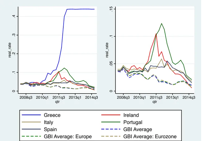
country order is barely changed in terms of the average rate and maximum realized rate for each country (Figure 1.13). Finally, Figure 1.14 reports the sovereign rates of the distressed European economies relative to several GBI averages during the European debt crisis. Clearly Greece experienced an exorbitant hike reflected in the Greek GBI index. Greece’s interest spike is followed by Portugal and Ireland’s and to a lesser extent by Spain and Italy. The GBI average excluding the distress economies are actually decreasing. As a robustness check (reported in a subsequent section), I discuss excluding the GIIPS from the analysis.

1.5

Identification

The widely accepted identification outlined by Blanchard and Perotti (2002) uses institutional knowledge. The paper as well as much of the subsequent literature con-strain the government to respond to macroeconomic fundamentals with at least a quarter delay. In other words within a period, the government cannot respond to macroeconomic fundamentals. The assumption is justified by pointing out institu-tional delays in implementing fiscal changes. The delays are related to both collecting data on the private sector as well as legislating and executing fiscal reforms. For this reason the use of quarterly data is essential. This identification can be recast as an A model outlined in detail in Lutkepohl (2007). In particular I assume that the observed

(31)

relationships in the data can be modeled as a stationary VAR of order p:

yt=A1yt 1+....+Apyt p+ut

yt is a vector



gt gdpt it tbyt rtus Rt

gtis government consumption,gdpt is output,itis in investment,tbytis trade balance

relative to GDP, rus

t is the world safe rate proxy and Rt is the sovereign interest rate.

All variables are expressed in real terms.

Further I assume that there is an A matrix such that:

Ayt =A⇤1yt 1+...+A⇤pyt p+et

where et is a vector of orthogonal structural shocks with a diagonal ⌃e covariance

matrix. The assumption implies the A-model formulation:

Aut =et

with AAi = A⇤i. After imposing appropriate restrictions on A we can bring the

following system to the data:

yt= [I A]

| {z }

Aestimate

yt+A⇤1yt 1+...+A⇤pyt p+et

Finally I can express yt in terms of orthogonal shocks:

yt = 1 X i=0 iut i = 1 X i iA 1Aut i = 1 X i ✓iet i

(32)

with ⇥i = iA 1

The restriction I impose on A are based on Blanchard and Perotti (2002) for the public sector part of the model and on Uribe and Yue (2006) for the macroeconomic fundamentals. Uribe and Yue (2006) propose the identification I employ and verify that it is consistent with the canonical IRBC model of a small open economy. In par-ticular their identification assumes that the interest rates respond to fundamentals within quarter while fundamental respond with 1 quarter delay. The restrictions are as follows: ug_t =eg_t ugdp_t =a21ugt +e y t ui t=a31ugt +a32ugdpt +eit utbyt =a41ugt +a42ugdpt +a43uit+e tby t urus t =ert uR t =a61ugt +a62ugdpt +a63uit+a64utbyt +a65rust +eRt 2 6 6 6 6 6 6 6 6 6 6 6 6 6 6 4 1 0 0 0 0 0 a21 1 0 0 0 0 a31 a32 1 0 0 0 a41 a42 a43 1 0 0 0 0 0 0 1 0 a61 a62 a63 a64 a65 1 3 7 7 7 7 7 7 7 7 7 7 7 7 7 7 5 u=et

I assume that a country cannot single-handedly influence the world safe rate. Hence

the impact and lagged feedback coefficients are set to 0. The literature is in general

(33)

studying both emerging and developed economies in parallel to establish di↵erences in their behavior, I have to consider to what extent this is a justifiable assumption. Ultimately we are looking for a measure of global factors i.e. a variable which has

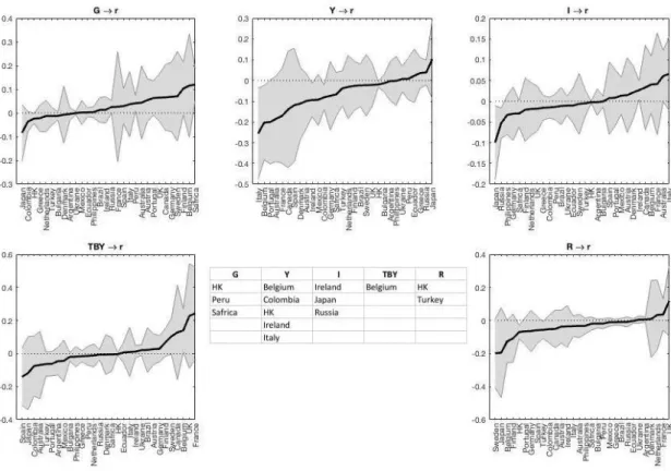
the same realization in all countries per time period.20 _{Figure 1.16 displays}

Graner-causality test. The figure shows the coefficient for each country in the system. For the

vast majority of countries we cannot reject the null that the country fundamentals

do not a↵ect the safe rate. The ”exceptions” are not the countries we would have

expected so I attribute the rejection of the null to the short time series.

The panel structure of the data allows us to get around the sparsity of individual country data. Data on fiscal variables as well as aggregate demand variables start mostly in the early 1990s. Apart from this consideration, the coverage of the EMBI and the GBI indices also imposes a similar constraint on the individual time series data. The dataset includes 84 quarters per country with some missing data for

in-dividual countries. This is by no means sufficiently long time-series to assure us in

the validity of the estimates. This problem is alleviated by the panel dimension. At the same time, the panel structure of the data posits the challenge of dealing with cross-country heterogeneity. I follow the panel VAR literature in assuming that the dynamic response for a country are the same up to randomly distributed country specific fixed e↵ect:

uit=µi+⌫it

It is further assumed that the two disturbance components are mean 0 and orthogonal to each other.

E(µi) = E(⌫it) =E(µi⌫it) = 0

20_{In the dynamic panel (GMM) exercise the data has been deseasonalized only as the main} equa-tion is specified in first di↵erences, while for the FE e↵ect estimation, I use linearly detrended and deseasonalized data. Estimates are extremely close if I quadratically detrend or if I use detrended data for the GMM exercise.

(34)

withi₂1 :N andt ₂1 :T. The presence of a fixed country e↵ect would bias pooled

estimates of the system’s coefficients.21 _{Lagged dependent variables in the system}

raise concern about the fixed e↵ect estimator su↵ering from Nickell bias (Nickell

(1981)) i.e. the demeaned lagged regressors being correlated with the demeaned dis-turbances. For this purpose I employ dynamic panel estimation. In particular I use

the di↵erence GMM estimator: the equations are estimated in first di↵erence with lags

of the regressors used as instruments. First di↵erencing the equations expunges the

fixed e↵ect. However, it introduces the problem that the first di↵erenced disturbances

(₄uit=uit uit 1) are endogenous to the lagged regressors (4yit 1 =yit 1 yit 2).

To address this issue the di↵erence GMM uses past realizations of the lagged

depen-dent variables to instrument for the endogenous first-di↵erenced regressors withyt T,

T ₂2...t 1 being all valid instruments in the absence of first order autocorrelation in

⌫it. 22 I choose to use three lags of instruments and verify that the results are robust

to using fewer or more instruments. To verify the validity of the instruments used in the GMM estimation, I report the Sargan / Hansen test for joint validity as well as the Arellano and Bond test for autocorrelation in the idiosyncratic disturbance

⌫it. Since 4uit is correlated with 4uit 1 by construction, testing for second order

autocorrelation in the di↵erenced errors is a valid test for first order autocorrelation

in the residuals in levels.23 _{Both the Sargan / Hansen test and the Arellano and}

Bond test confirm that the matrices yt p i for i2[1 : 3] are valid instruments. Only

for the investment equations is the null of no first order autocorrelation rejected. To

alleviate this concern, I also report estimates of the third row of the Ai matrices

using alternative dynamic panel estimators.24_,25 _{While the dynamic panel estimators}

21_{The bias would be less important, the longer is the time series.}

22_{Autocorrelation in the error would force us to truncate the sequence of appropriate instruments.} 23_{Autocorrelation test p+1 on the di}_↵_{erenced residuals tests for p correlation in the residuals in} levels.

24_{The Arellano Bond test statistic in constructed under the assumption of large N and small T} as well as E(eitejt) = 0. Controlling for the safe rate helps with the latter assumption, but the

relatively small N in the empirical sample (N = 30) might be problematic.

(35)

are less taxing in terms of degrees of freedom loss due to deeper-lag instruments, the

time series length (T = 82) in the data is perhaps sufficient to make the dynamic

bias small and to justify the use of a more straightforward estimation technique such

as the fixed e↵ect estimator. In turns out that in this particular empirical

specifi-cation the fixed e↵ect estimates of the system lead to instability issues. Empirically

I demonstrate that the distressed European economies as a group are the potential

culprit. Excluding them indeed fixes the problem. I report fixed e↵ect estimation for

the sample excluding this group (GIIPS: Greece, Italy, Ireland, Portugal, Spain) as a robustness check.

Finally in order to estimate di↵erences in dynamic responses between developed and

emerging economies I modify the estimation to include an emerging-dummy interac-tion26_:

al,ij = ˜al,0(ij) + ˜al,1(ij)⇥ [EM E]

al,ij is the ij-th element ofAl for l 2[0..p] and EME selects the emerging economies

in the sample.

The AIC criterion selects one lag as optimal (see Figure 1.37). The autoregressive

coefficients for the safe rate are estimated by OLS in first di↵erences.

1.6

SVAR Analysis

Figure 1.31 and figure 1.32 show the GMM estimates of the system for both the de-veloped and the emerging group. Figure 1.33 explicitly focuses on the government

(2009).

26_{This is equivalent to estimating the system separately for each group, but leads to a slight} efficiency improvement.

(36)

response. Overall, the government responds pro-cyclically to output for both groups. The point estimates suggest that worsening international financial conditions decrease government consumption. Increases in the safe rate as well as the sovereign interna-tional borrowing rate lead to a decrease in government consumption for both groups. Both the group by group estimates and the joint estimates suggest that emerging economies are more mindful of international credit constraints and decrease govern-ment consumption in response to an increase in the safe borrowing rate and their own sovereign borrowing rate. Conversely, international credit constraints have a lower bite for governments in developed economies vis-`a-vis those in emerging economies. Moreover, the government response to output is similar for the two groups and statis-tically indistinguishable. This juxtaposition sheds light on one of the main questions of the paper: whether emerging governments are more sensitive to the cycle and whether they respond more pro-cyclically to output fluctuations. Conditional on my identification, it turns out this is not the case.

Figure 1.34 reports results for the government response function estimated using private GDP instead. I confirm that emerging governments decrease consumption expenditure in response to increases in the borrowing rate they face on international

markets. This is still the main di↵erence between the two government response

func-tions. If anything, the coefficient on the interest rate is even higher in magnitude

when private GDP is used in the estimation. This is also the case with FE estimates

(figure 1.35). The FE estimation confirms that the main di↵erence between emerging

and developed economies stems from their response to the sovereign rate. Di↵erently

from GMM, the fixed e↵ect estimation suggests that government consumption does

not respond to GDP fluctuations at all. The coefficient on real GDP is lower and

imprecisely estimated. In the next section I show that the bootstrapped impulse re-sponse still implies an increase in government consumption following a positive output

(37)

shock even in the FE estimation case. Finally, figure 1.36 shows another robustness

check for the government response function. In particular, I report fixed e↵ect

esti-mates for a country subset which excludes Greece, Portugal and Italy. Greece and Portugal are the countries experiencing the largest increase in government yields rel-ative to the rest of several subsets of the GBI index family during the European debt crisis. I choose to report this particular cut of the data because excluding all of the distressed European economies leads to stability issues in the VAR analysis. I revisit this issues in the robustness section. I exclude Greece, Portugal and Italy and re-estimate the system with FE. I also report results from GMM estimation which excludes all distressed European economies (Greece, Portugal, Ireland, Italy and Spain). This particular GMM estimation should be interpreted with care, be-cause further decreasing the number of panels raises concerns. In the GMM case, the

di↵erence between the full sample and the sub-sample for the developed group is that

the coefficient on the lagged dependent variable increases and there is no response of

government consumption to fundamentals apart from that to the safe rate. For the emerging group the GMM estimates on the subset suggest just the opposite: govern-ment consumption is less persistent and more responsive to fundagovern-mentals relative to

emerging. The fixed e↵ect estimates on the full sample and subsample are quite

sim-ilar. In both FE exercises governments do not respond to fundamentals apart from the sovereign rate. Increases in the international sovereign rate are contractionary for both the full sample and the subset albeit imprecisely estimated in the subsample case.

Returning to the rest of the variables in the model (figure 1.31 & figure 1.32), we

already see that the efficacy of government consumption as a policy instrument is

substantially lower as captured by the impact coefficient on GDP. As anticipated

an increase in government consumption is expansionary. However, as the coefficient

(38)

economies is a third that for developed. The crowding-out of investment on the other

hand by government consumption is lower in emerging economies. The coefficient on

L.GC is practically o↵-set by the coefficient on L.GC_⇥I(Emerging) for investment.

Al-though the current analysis does not include measures of how the government finances government expenditure, the lack of crowding out for investment is symptomatic of revenue financed increases in government expenditure for emerging economies, which can be one factor behind the lower multiplier for this group (I discuss the multiplier in the next section). The estimates suggest that government consumption leads to a greater deterioration in the trade balance for developed economies which is consistent with either a greater share of imported goods and services in the government con-sumption basket or a stronger multiplier on private sector concon-sumption. Finally, for either group fluctuations in government consumption do not impact directly sovereign borrowing constraints.

As anticipated, investment is strongly pro-cyclical for both emerging and developed.

The trade balance is again as anticipated counter-cyclical due to the e↵ect of

invest-ment as emphasized by the IRBC. Sovereign credit constraints do not directly a↵ect

fundamentals except in the case of investment for developed economies. On the other hand the sovereign rate shows a lot of persistence for developed economies and less so for emerging. As a matter of fact I estimate a significant feedback from output to the sovereign borrowing rate for emerging and not for developed. The sovereign rate is less persistent in the case of emerging economies. To capture the rich dynamics of the system I discuss the impulse response analysis in the next section.

(39)

1.6.1

Impulse Responses

Shocks to Government Consumption

Figure 1.17 reports the impulse response to a unitary orthogonal shock to government consumption expenditure. Government consumption expenditure is expansionary for both emerging and rich economies. For the rich group there is a greater evidence of investment crowding out during the initial quarters for which the impulse response is statistically indistinguishable from 0. For subsequent quarters developed economies investment is higher but the impulse responses for the two groups are still

statisti-cally indistinguishable from each other. The e↵ectiveness of government consumption

in stimulating output is ostensibly higher for the developed group. Government con-sumption shocks cause a slight deterioration in the trade balance. Finally the response of the interest rate is the mirror image for the two groups with borrowing conditions improving for emerging economies in response to a government consumption shock. As we saw in the estimates of the system the response of the borrowing rate is de-termined by the response of the rate to output fluctuations rather than the directly through government consumption. Finally there is no response of the world safe rate

by construction. As the persistence of government consumption di↵ers between the

2 groups I calculate the multiplier next.

Figure 1.18 reports the government consumption multiplier. Following the literature, I define the government consumption spending multiplier as:

impact multiplier = 4X0 4G0 cumulative multiplier = PT t=04Xt PT t=04Gt

(40)

Xt2



gt gdpt it tbyt rust Rt

Normally the literature reports the multiplier e↵ect of government (consumption)

expenditure on GDP. To facilitate the comparison between the two groups, I report

the multiplier e↵ect of shocks on all variables in the system. There is a striking

dif-ference between the multiplier e↵ect of government consumption on output in the

two groups. In emerging economies government consumption is substantially less ef-fective in stimulating output; the impact multiplier is roughly two times lower than the impact multiplier for developed economies. For both groups the multiplier is less than 1, which is consistent with estimates of the multiplier in Ilzetzki et al. (2013).

However, di↵erently from them I do not obtain negative multipliers. I do not find

di↵erence in the two groups for the investment multiplier which is consistent with

bigger crowding out for the developed group. The deterioration in the trade bal-ance is of similar magnitude for both groups. Finally, as fundamentals improve, the sovereign borrowing rate also improves for emerging economies. On impact, a unitary increase in government consumption leads to a 16 basis points decrease in the rate.

The cumulative multiplier e↵ect is as high as 12%. In other words, a 10% increase in

government consumption decreases the sovereign borrowing rate by 1.23% for

emerg-ing economies and while the same increase in government consumption would induce an increases in the rate by 73 basis points for developed over the whole cycle. Fig-ure 1.18 also reports the government consumption multiplier on private GDP. The comparison between the two groups still holds with the short-run multipliers being up to 3 times lower and the long run multiplier up to 2 times lower for emerging

economies. It should be noted that estimates deal with officially reported GDP. If we

(41)

multiplier for the informal sector would be also very informative.

Shocks to Output

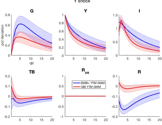
Next I consider shocks to output. Figure 1.19 reports the response of the variables in the model to a unitary shock to output. The empirical responses are consistent with the predictions of the SOE IRBC model: investment responds more than one for one with output and the trade balance is countercyclical. The impact response of investment in emerging economies is slightly higher. However the investment re-sponse converges to being indistinguishable between emerging and rich as the horizon increases. One of the key questions I am after is whether emerging governments

respond di↵erently to output fluctuations; in particular whether government

con-sumption expenditure re-enforces the cycle. While the median response for emerging governments is higher, the response of government consumption to output fluctuation is indistinguishable from the developed group’s. This results suggests that emerging governments do not necessarily have a more pro-cyclical stance. Instead as revealed by the response to interest rate shocks which is to be discussed next, government consumption expenditure is more sensitive to sovereign interest rate shocks. The sovereign rate responds to fundamentals in emerging economies while the response in developed is statistically indistinguishable from 0. Figure 1.20 reports the multiplier

e↵ect of an output shock on the rest of the model variables. The median multiplier

e↵ect of output on government consumption is higher- between 4 to 24 percentage

points, in emerging economies. Given that the coefficients on the response function

are the same, the higher multiplier is due to the fact that the increase in output relaxes the borrowing constants for emerging governments. In other words, emerging governments raise government consumption in response to a positive output shock because of the relaxed international borrowing constraints. In particular in emerg-ing economies the median impact improvement in the government interest rate is 14

(42)

percentage points and the long run improvement- 33 percentage points. For the de-veloped group the improvement in the long run is roughly 1 percentage point and is not statistically significant.

Shocks to the Sovereign Borrowing Rate

Figure 1.21 reports the impulse response of the model variables to a unitary shock in the sovereign borrowing rate. The shock leads to a contraction in emerging economies albeit a milder one relative to the estimates in Uribe and Yue (2006) and Akinci (2013). The developed group can weather the shock without a significant decrease in the government consumption or output. However, for the developed group, there is a substantial decrease in investment and an improvement in the trade balance. To

account for the di↵erence in persistence of the shock propagation I recast the impulse

response in a multiplier form as shown in figure 1.22. The median multiplier for emerging governments’ consumption to an interest rate shock is twice as high as that for developed. The median response for output is twice as high. However, as noted before investment in developed economies responds twice as strongly to an interest rate shock as investment in the emerging group.

Shocks to the Safe Rate

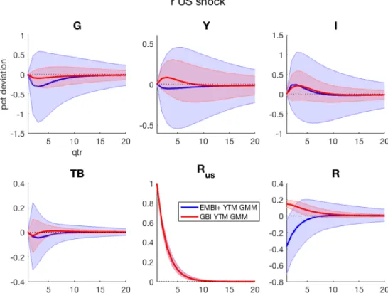
Figure 1.23 displays the impulse responses to a unitary shocks to the safe rate. As

the autoregressive process for the safe rate (0.992 in level and 0.596 in di↵erence) is

close to non-stationary I report estimates with the rate in di↵erences. The safe rate

shocks matter mostly for the international borrowing rate faced by sovereigns with a limited implication for other fundamentals. This is consistent with the findings of Akinci (2013) who also finds that the global safe rate is the least important among the international financial conditions she considers. It should be noted that an increase in the safe rate decreases the sovereign rate for emerging and increases the sovereign

(43)

rate for developed. My results concur with the analysis of Eichengreen and Mody (1998), which focuses on first issuance emerging markets spreads in the early 90s.

The sign of the e↵ect depends on whether supply or demand e↵ects are stronger on

net. On the one hand a fall in the US treasury rate shifts investor demand towards

bond markets which o↵er a higher yield. The demand e↵ect will lead to a same sign

movement in the safe rate and the sovereign rate. On the other hand as shown by Eichengreen and Mody (1998) an increase in the US rate decreases the likelihood of a bond issuance in emerging markets which in turn limits the supply and leads to a decrease in the bond rate. Therefore, the impulse response suggest that the supply

e↵ects are leading when it comes to emerging sovereign bonds. As I do not have

direct evidence on the dependence of issuance on the US rate for developed sovereign bonds, we I only conjecture that their issuance probability is either less sensitive to

the US rate or that demand e↵ec