Valuation using multiples. How do analysts reach their conclusions?

Full text

(1)IESE UNIVERSITY OF NAVARRA. VALUATION USING MULTIPLES. HOW DO ANALYSTS REACH THEIR CONCLUSIONS?. Pablo Fernández*. RESEARCH PAPER No 450 January, 2002. *. Professor of Financial Management, IESE. Research Division. IESE University of Navarra Av. Pearson, 21 08034 Barcelona - Spain. Copyright © 2002, IESE Do not quote or reproduce without permission.

(2) VALUATION USING MULTIPLES. HOW DO ANALYSTS REACH THEIR CONCLUSIONS?. Abstract This paper focuses on equity valuation using multiples. Our basic conclusion is that multiples nearly always have broad dispersion, which is why valuations performed using multiples may be highly debatable. We revise the 14 most popular multiples and deal with the problem of using multiples for valuation: their dispersion. 1,200 multiples from 175 companies illustrate the dispersion of multiples of European utilities, English utilities, European constructors, hotel companies, telecommunications, banks and Internet companies. We also show that PER, EBITDA and Profit after Tax (the most commonly used parameters for multiples) were more volatile than equity value during the period 1991-99. We also provide additional evidence of the analysts’ recommendations for Spanish companies: less than 15% of the recommendations are to sell. However, multiples are useful in a second stage of the valuation: after performing the valuation using another method, a comparison with the multiples of comparable firms enables us to gauge the valuation performed and identify differences between the firm valued and the firms it is compared with.. JEL Classification: G12, G31, M21 Keywords: multiples, dispersion of multiples, PER, relative multiples, analysts’ recommendations.. (1) I would like to thank Laura Reinoso and Laura Parga for their impressive work with data collection and Charlie Porter for his wonderful help revising earlier drafts of this paper..

(3) VALUATION USING MULTIPLES. HOW DO ANALYSTS REACH THEIR CONCLUSIONS?. This paper focuses on equity valuation using multiples. The basic conclusion is that multiples almost always have broad dispersion, which is why valuations performed using multiples are highly debatable. However, multiples are useful in a second stage of the valuation: after performing the valuation using another method, a comparison with the multiples of comparable firms enables us to gage the valuation performed and identify differences between the firm valued and the firms it is compared with.. 1. Valuation methods used by the analysts Figure 1 shows the valuation methods (2) most widely used by Morgan Stanley Dean Witter’s analysts for valuing European companies. Surprisingly, the discounted cash flow (DCF) is in fifth place, behind multiples such as the PER, the EV/EBITDA and the EV/EG. Figure 1. Most widely used valuation methods PER to Growth EV/Plant EV/FCF. Percentage of analysts that use each method. P/Sales EV/Sales P/CE FCF P/BV DCF EV/EG Residual Income EV/EBITDA PER 0%. 10%. 20%. 30%. Source: Morgan Stanley Dean Witter Research. (2) Weighted by the market capitalization of the industry in which it is applied.. 40%. 50%.

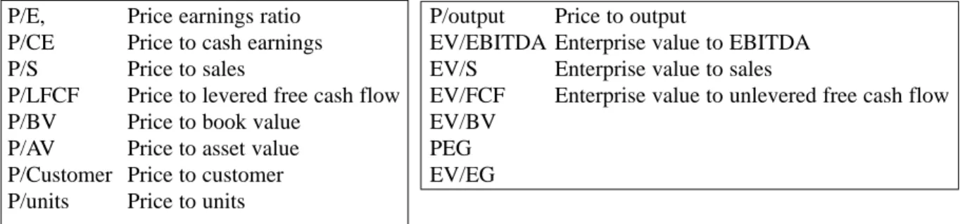
(4) 4. 2. Most commonly used multiples Although as Figure 1 shows, the PER and the EV/EBITDA seem to be the most popular multiples for valuing firms, it is also true that, depending on the industry being analyzed, certain multiples are more appropriate than others. Table 1. Most commonly used multiples. P/E, P/CE P/S P/LFCF P/BV P/AV P/Customer P/units. Price earnings ratio Price to cash earnings Price to sales Price to levered free cash flow Price to book value Price to asset value Price to customer Price to units. P/output EV/EBITDA EV/S EV/FCF EV/BV PEG EV/EG. Price to output Enterprise value to EBITDA Enterprise value to sales Enterprise value to unlevered free cash flow. The multiples can be divided into three groups (3): 1. Multiples based on the company’s capitalization (equity value: E). 2. Multiples based on the company’s value (equity value and debt value: E+D) (4). 3. Growth-referenced multiples. 2.1. Multiples based on capitalization The price- or capitalization-based multiples have the advantage of being very easy to understand and calculate. 1. Price Earnings Ratio (PER). PER = market capitalization / total net income = share price / earnings per share Sometimes, the mean of last or next few years’ earnings is used. 2. Price to Cash Earnings (P/CE). P/CE = market capitalization / (net income before depreciation and amortization) 3. Price to sales (P/S). P/S= market capitalization / sales = Share price / sales per share. (3) Morgan Stanley Dean Witters Report How We Value Stocks, 15 September 1999. (4) The value of the firm (E+D) is often called Enterprise Value (EV). However, the initials are also used sometimes to indicate the value of the shares (Equity Value)..

(5) 5. This multiple compares sales with capitalization (the shares’ value) only. However, sales are attributable to all the company’s stakeholders: shareholders, creditors, pensioners, Inland Revenue... As we will see in the next paper, this multiple is often used to value Internet companies... and also telecommunications infrastructure companies, bus companies and pharmacies. 4. Price to Levered Free Cash Flow (P/LFCF). P/LFCF= Market capitalization / (Operating income after interest and tax + depreciation + amortization – increased working capital requirements – investments in existing businesses (5)). One variant of this multiple is the P/FAD (funds available for distribution). 5. Price to Book Value (P/BV). VM/VC = P/BV= market capitalization / book value of shareholder’s equity In a firm with constant growth g, the relationship between market value and book value is: P/BV= (ROE-g)/ (Ke-g) This multiple is often used to value banks. Other industries that use P/BV or its derivatives are the paper and pulp industry, real estate and insurance. One variant of this multiple for the insurance industry is the capitalization / embedded value (shareholder’s equity + present value of the future cash flows on signed insurance contracts). 6. Price to Customer P / Customer = market capitalization / number of customers This multiple is very commonly used to value cellular phone and Internet companies. 7. Price to units This multiple is often used to value soft drinks and consumer product companies. 8. Price to output This multiple is used to value cement and commodities companies.. (5) “Investments in existing businesses” are those in businesses that the company already has. They do not include growth-oriented investments, either for new businesses or to increase capacity..

(6) 6. 9. Price to potential customer As we will see in the next paper, some analysts use this multiple to value Internet companies. 2.2. Multiples based on the company’s value These multiples are similar to those in the previous section, but instead of dividing the market capitalization by another parameter, they use the sum of the firm’s market capitalization and financial debt. This sum is usually called the Enterprise Value (EV) (6). 1. Enterprise Value to EBITDA (EV/EBITDA). EV/ EBITDA = Enterprise value / Earnings before interest, tax, depreciation and amortization. This is one of the most widely used multiples by analysts. However, the EBITDA (earnings before interest, tax, depreciation and amortization) has a number of limitations (7), including: 1. It does not include the changes in the working capital requirements (WCR) 2. It does not consider capital investments. 2. Enterprise Value to Sales (EV/Sales). EV/Sales = Enterprise value / Sales.. 3. Enterprise Value to Unlevered Free Cash Flow (EV/FCF). EV/FCF = Enterprise value / (Earnings before interest and after tax + depreciation + amortization - increased working capital requirements - capital investments (8)).. 2.3. Growth-referenced multiples 1. P/EG or PEG. PER to EPS growth PER/g = P/EG = PEG = PER / growth of earnings per share in the next few years. (6) If there are preferred shares and minority interests, the enterprise value is: market capitalization + preferred shares + minority interests + net debt. (7) For a good report on the limitations of the EBITDA, see Putting EBITDA In Perspective, Moody’s Investors Service, June 2000. (8) Sometimes recurrent free cash flow is used as well. In this case, investments in existing businesses are considered..

(7) 7. This multiple is mainly used in growth industries, such as luxury goods, health and technology. 2. EV/EG. Enterprise value to EBITDA growth EV/ EG= EV/EBITDA (historic) / growth of EBITDA in the next few years As with the previous multiple, it is mainly used in growth industries, particularly health, technology and telecommunications.. 3. Relative multiples All of these multiples by themselves can tell us very little. They need to be placed in a context. There are basically three relative valuations: 1. With respect to the firm’s own history 2. With respect to the market 3. With respect to the industry 1. With respect to the firm’s history History-referenced multiple = multiple / mean of recent years’ multiple One problem with historic multiples is that they depend on exogenous factors, such as interest rates and stock market situation. In addition, the composition and nature of many firms’ business changes substantially over time, so it does not make much sense to compare them with previous years. 2. With respect to the market Market-referenced multiple = firm multiple / market multiple 3. With respect to the industry Industry-referenced multiple = firm multiple / industry multiple This comparison with the industry is more appropriate than the two previous comparisons. However, one problem is that when the industry is overvalued, all of the companies in it are overvalued: a clear example of this situation was the Internet companies up to 2000. We shall also see in section 4 that the multiples of companies operating in the same industry normally have very wide dispersion..

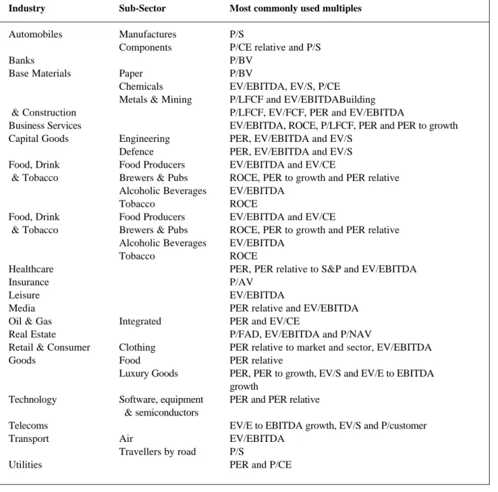
(8) 8. Table 2 is a summary of the most commonly used multiples for valuing different industries. Table 2. Most commonly used multiples in different industries Industry. Sub-Sector. Most commonly used multiples. Automobiles. Manufactures Components. P/S P/CE relative and P/S P/BV P/BV EV/EBITDA, EV/S, P/CE P/LFCF and EV/EBITDABuilding P/LFCF, EV/FCF, PER and EV/EBITDA EV/EBITDA, ROCE, P/LFCF, PER and PER to growth PER, EV/EBITDA and EV/S PER, EV/EBITDA and EV/S EV/EBITDA and EV/CE ROCE, PER to growth and PER relative EV/EBITDA ROCE EV/EBITDA and EV/CE ROCE, PER to growth and PER relative EV/EBITDA ROCE PER, PER relative to S&P and EV/EBITDA P/AV EV/EBITDA PER relative and EV/EBITDA PER and EV/CE P/FAD, EV/EBITDA and P/NAV PER relative to market and sector, EV/EBITDA PER relative PER, PER to growth, EV/S and EV/E to EBITDA growth PER and PER relative. Banks Base Materials. & Construction Business Services Capital Goods Food, Drink & Tobacco. Food, Drink & Tobacco. Healthcare Insurance Leisure Media Oil & Gas Real Estate Retail & Consumer Goods. Technology Telecoms Transport Utilities. Paper Chemicals Metals & Mining. Engineering Defence Food Producers Brewers & Pubs Alcoholic Beverages Tobacco Food Producers Brewers & Pubs Alcoholic Beverages Tobacco. Integrated Clothing Food Luxury Goods Software, equipment & semiconductors Air Travellers by road. EV/E to EBITDA growth, EV/S and P/customer EV/EBITDA P/S PER and P/CE. Table 3 shows the average multiple of different industries (9) in the US stock market in September 2000. The total number of companies analyzed was 5,903..

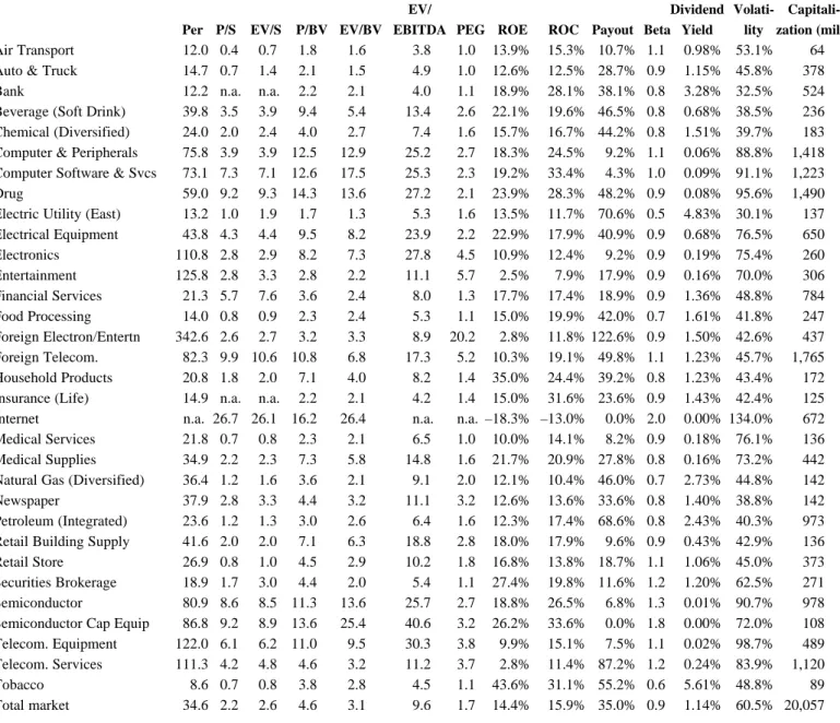
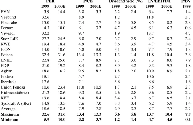
(9) 9. Table 3. Mean multiples of different American industries. September 2000.. Per P/S. Air Transport Auto & Truck Bank Beverage (Soft Drink) Chemical (Diversified) Computer & Peripherals Computer Software & Svcs Drug Electric Utility (East) Electrical Equipment Electronics Entertainment Financial Services Food Processing Foreign Electron/Entertn Foreign Telecom. Household Products Insurance (Life) Internet Medical Services Medical Supplies Natural Gas (Diversified) Newspaper Petroleum (Integrated) Retail Building Supply Retail Store Securities Brokerage Semiconductor Semiconductor Cap Equip Telecom. Equipment Telecom. Services Tobacco Total market. EV/S. EV/ P/BV EV/BV EBITDA PEG ROE. 12.0 0.4 0.7 1.8 14.7 0.7 1.4 2.1 12.2 n.a. n.a. 2.2 39.8 3.5 3.9 9.4 24.0 2.0 2.4 4.0 75.8 3.9 3.9 12.5 73.1 7.3 7.1 12.6 59.0 9.2 9.3 14.3 13.2 1.0 1.9 1.7 43.8 4.3 4.4 9.5 110.8 2.8 2.9 8.2 125.8 2.8 3.3 2.8 21.3 5.7 7.6 3.6 14.0 0.8 0.9 2.3 342.6 2.6 2.7 3.2 82.3 9.9 10.6 10.8 20.8 1.8 2.0 7.1 14.9 n.a. n.a. 2.2 n.a. 26.7 26.1 16.2 21.8 0.7 0.8 2.3 34.9 2.2 2.3 7.3 36.4 1.2 1.6 3.6 37.9 2.8 3.3 4.4 23.6 1.2 1.3 3.0 41.6 2.0 2.0 7.1 26.9 0.8 1.0 4.5 18.9 1.7 3.0 4.4 80.9 8.6 8.5 11.3 86.8 9.2 8.9 13.6 122.0 6.1 6.2 11.0 111.3 4.2 4.8 4.6 8.6 0.7 0.8 3.8 34.6 2.2 2.6 4.6. 1.6 1.5 2.1 5.4 2.7 12.9 17.5 13.6 1.3 8.2 7.3 2.2 2.4 2.4 3.3 6.8 4.0 2.1 26.4 2.1 5.8 2.1 3.2 2.6 6.3 2.9 2.0 13.6 25.4 9.5 3.2 2.8 3.1. 3.8 4.9 4.0 13.4 7.4 25.2 25.3 27.2 5.3 23.9 27.8 11.1 8.0 5.3 8.9 17.3 8.2 4.2 n.a. 6.5 14.8 9.1 11.1 6.4 18.8 10.2 5.4 25.7 40.6 30.3 11.2 4.5 9.6. 1.0 1.0 1.1 2.6 1.6 2.7 2.3 2.1 1.6 2.2 4.5 5.7 1.3 1.1 20.2 5.2 1.4 1.4 n.a. 1.0 1.6 2.0 3.2 1.6 2.8 1.8 1.1 2.7 3.2 3.8 3.7 1.1 1.7. Dividend Volati- CapitaliROC Payout Beta Yield lity zation (mill.). 13.9% 15.3% 10.7% 1.1 12.6% 12.5% 28.7% 0.9 18.9% 28.1% 38.1% 0.8 22.1% 19.6% 46.5% 0.8 15.7% 16.7% 44.2% 0.8 18.3% 24.5% 9.2% 1.1 19.2% 33.4% 4.3% 1.0 23.9% 28.3% 48.2% 0.9 13.5% 11.7% 70.6% 0.5 22.9% 17.9% 40.9% 0.9 10.9% 12.4% 9.2% 0.9 2.5% 7.9% 17.9% 0.9 17.7% 17.4% 18.9% 0.9 15.0% 19.9% 42.0% 0.7 2.8% 11.8% 122.6% 0.9 10.3% 19.1% 49.8% 1.1 35.0% 24.4% 39.2% 0.8 15.0% 31.6% 23.6% 0.9 –18.3% –13.0% 0.0% 2.0 10.0% 14.1% 8.2% 0.9 21.7% 20.9% 27.8% 0.8 12.1% 10.4% 46.0% 0.7 12.6% 13.6% 33.6% 0.8 12.3% 17.4% 68.6% 0.8 18.0% 17.9% 9.6% 0.9 16.8% 13.8% 18.7% 1.1 27.4% 19.8% 11.6% 1.2 18.8% 26.5% 6.8% 1.3 26.2% 33.6% 0.0% 1.8 9.9% 15.1% 7.5% 1.1 2.8% 11.4% 87.2% 1.2 43.6% 31.1% 55.2% 0.6 14.4% 15.9% 35.0% 0.9. 0.98% 1.15% 3.28% 0.68% 1.51% 0.06% 0.09% 0.08% 4.83% 0.68% 0.19% 0.16% 1.36% 1.61% 1.50% 1.23% 1.23% 1.43% 0.00% 0.18% 0.16% 2.73% 1.40% 2.43% 0.43% 1.06% 1.20% 0.01% 0.00% 0.02% 0.24% 5.61% 1.14%. 53.1% 64 45.8% 378 32.5% 524 38.5% 236 39.7% 183 88.8% 1,418 91.1% 1,223 95.6% 1,490 30.1% 137 76.5% 650 75.4% 260 70.0% 306 48.8% 784 41.8% 247 42.6% 437 45.7% 1,765 43.4% 172 42.4% 125 134.0% 672 76.1% 136 73.2% 442 44.8% 142 38.8% 142 40.3% 973 42.9% 136 45.0% 373 62.5% 271 90.7% 978 72.0% 108 98.7% 489 83.9% 1,120 48.8% 89 60.5% 20,057. 4. The problem with multiples: their dispersion. 4.1. Dispersion of the utilities’ multiples Table 4 shows multiples used to value European utilities. Table 5 concentrates solely on English utilities. Note the multiples’ wide dispersion in all cases..

(10) 10. Table 4. Multiples of European utilities (excluding the English utilities). September 2000. PER 1999 2000E. P/CE 1999 2000E. EVN Verbund Electrabe Fortum Vivendi Suez LdE RWE E.ON Edison ENEL EDP Agbar Endesa Iberdrola Unión Fenosa Hidrocantábrico REE Sydkraft A (SKr) Average. –5.9 32.6 15.0 4.3 32.2 27.2 19.4 14.0 32.5 22.8 21.0 18.6 18.1 17.6 10.6 21.2 19.6 14.8 18.6. 14.4. 23.4 18.6 18.4 13.3 18.5. 3.8 8.9 7.4 6.1 9.7 6.8 4.9 5.8 13.4 7.7 8.4 9.5 5.7 7.1 11.0 9.3 8.8 7.6 7.9. Maximum Minimum. 32.6 –5.9. 31.6 10.0. 13.4 3.8. 15.1 10.0 24.5 18.4 10.6 31.6 25.6 19.2 16.2. 5.3. Dividend yield (%) EV/EBITDA 1999 2000E 1999 2000E. 2.4. 10.5 8.5 8.4 7.0 7.8. 2.2 1.2 5.6 4.7 1.9 2.7 3.6 3.1 1.3 2.7 3.9 1.8 2.7 3.6 1.7 2.6 3.4 3.3 2.9. 2.1 2.8 3.7 3.4 3.3. 6.4 11.8 8.5 6.1 13.7 9.7 4.7 7.7 11.8 7.3 9.3 10.9 10.6 8.6 7.5 9.6 6.7 6.2 8.7. 13.3 3.7. 5.6 1.2. 5.8 1.4. 13.7 4.7. 7.7 3.7 7.0 4.7 8.0 13.3 8.9 8.2 8.2. 6.9 8.5 6.5 5.9 7.7. 1.4 3.7 2.8 0.6 4.7 2.4 3.4 1.8 3.6 7.9 1.8 2.1 2.5 1.6 2.3 2.2 2.1 1.4 2.7. 10.4 4.5. 7.9 0.6. Dividend yield (%) EV/EBITDA 2000 2001E 2000 2001E. P/BV 2000. 5.8 4.5 2.9 3.9 3.4 1.4 3.0 4.2 2.0. 7.7. P/BV 1999. 8.2 6.3 8.3 4.5 7.9 10.4 8.6 9.3 8.9. Source: Morgan Stanley Dean Witter Research.. Table 5. Multiples of English utilities. September 2000. PER 2000 2001E. P/CE 2000 2001E. British Energy National Grid National Power PowerGen Scottish Power Scottish & Southern Anglian Water Hyder Kelda Pennon Severn Trent Thames United Utilities Average. 7.4 25.0 12.8 8.9 7.3 12.3 9.6 5.2 6.8 7.7 9.9 12.5 8.4 10.3. –26.1 29.8 14.7 7.4 18.2 12.4 12.0 5.0 10.6 11.9 10.9 27.7 12.1 11.3. 1.8 17.2 7.6 5.1 7.8 9.0 5.5 2.1 4.0 5.3 4.4 7.8 5.0 6.4. 2.4 14.7 8.9 5.1 8.7 8.9 5.8 2.2 4.8 6.3 4.9 11.7 6.0 7.0. 4.6 2.3 3.2 6.2 4.7 4.9 7.4 5.6 6.5 7.2 6.2 3.9 6.5 5.3. 4.6 2.5 3.4 6.8 5.0 5.1 7.6 5.9 6.9 5.4 6.5 4.1 6.7 5.4. 4.4 11.6 8.1 6.9 9.1 7.5 6.9 5.9 6.7 6.9 6.9 7.8 6.8 7.3. 5.7 11.4 10.0 6.3 7.6 7.6 7.1 5.2 7.1 7.9 6.3 8.6 7.3 7.5. 0.8 4.5 3.3 1.9 1.5 2.9 1.0 0.6 0.8 1.0 1.0 1.9 1.5 1.7. Maximum Minimum. 25.0 5.2. 29.8 –26.1. 17.2 1.8. 14.7 2.2. 7.4 2.3. 7.6 2.2. 11.6 4.4. 11.4 5.2. 4.5 0.6. Source: Morgan Stanley Dean Witter Research..

(11) 11. 4.2. Dispersion of the multiples of construction companies Table 6 shows different multiples for construction and building materials companies in Europe, America, Asia and Spain. Table 7 contains multiples for hotel companies Table 6. Multiples of construction companies. August 2000. PER 1999 2000E 2001 2002E. EV/EBITDA 1999 2000E 2001 2002E. 1999. CRH Holderbank Lafarge Saint Gobain Cemex Lafarge corporation Martin Marietta Materials Vulcan Materials Siam Cement Acciona ACS Dragados FCC Ferrovial Average. 17.5 19.5 15.2 18.0 5.5. 10.1 8.7 7.2 5.4 5.1. 7.6 7.6 5.9 4.6 5.7. 7.3 7.0 5.8 4.1 5.1. 7.0 6.5 5.5 3.7 4.9. 10.7 8.9 6.8 8.0 4.1. 8.8 8.2 6.1 5.9 5.0. 8.4 7.1 6.0 5.2 4.7. 8.0 6.6 5.7 4.7 4.5. 4.8. 4.7 7.2 2.7 3.2 11.5 10.6 9.6 5.7 8.3 7.1. 6.6 3.5 2.6 9.9 9.7 8.0 5.3 7.2 6.5. 2.3 9.0 8.8 7.6 5.1 6.3 6.2. Maximum Minimum. 11.5 2.7. 9.9 2.6. 9.0 2.3. 14.4 13.0 17.1 13.7 12.2 11.8 11.5 9.8 6.6 6.1. 12.4 12.2 10.2 8.4 5.7. 6.5. 6.0. 5.8. 5.3. 15.8 19.2 9.6 26.5 18.8 14.1 11.4 16.9 15.3. 15.0 17.0 6.6 22.3 15.3 13.6 11.3 13.0 13.0. 13.0 13.5 5.6 18.5 13.7 10.4 11.1 10.5 11.2. 16.1 12.1 9.1 10.6 9.2 10.6. 6.7 9.8 8.5 12.5 10.6 7.2 5.8 21.2 8.9. 6.2 5.6 8.9 7.5 5.7 5.1 9.1 7.8 7.8 7.1 6.5 5.9 5.6 5.3 16.2 14.2 7.3 6.6. 4.9 7.0 6.4 5.0 5.0 12.3 6.2. 7.9 2.4 4.1 15.4 12.4 9.6 6.1 10.1 8.2. 26.5 5.5. 22.3 18.5 6.0 5.6. 16.1 5.7. 21.2 5.1. 16.2 14.2 4.6 4.1. 12.3 37. 15.4 2.4. Source: Morgan Stanley Dean Witter Research.. Table 7. Multiples of hotel companies. November 2000. EV/EBITDA 2000E 2001E. Accor Bass Club Med Hilton Group Hilton Hotels Corp. Marriot Int’l Millenium & Copthorne NH Hotels Scandic Hotels Sol Meliá Starwood Thistle Hotels Average Maximum Minimum. PER 2000E. 2001E. 10.0 5.8 10.5 10.0 7.6 10.6 8.7 12.8 7.7 10.0 7.4 8.1. 9.0 6.3 8.2 8.8 7.3 9.4 8.0 9.9 6.5 8.7 7.1 7.8. 23.1 11.8 26.2 13.2 13.5 20.5 11.2 21.4 15.2 17.6 16.0 9.2. 20.0 10.7 18.4 11.4 12.8 18.4 9.8 18.1 14.5 14.4 14.2 9.2. 9.1 12.8 5.8. 8.1 9.9 6.3. 16.6 26.2 9.2. 14.3 20.0 9.2. P/CE 2000E 2001 2002E.

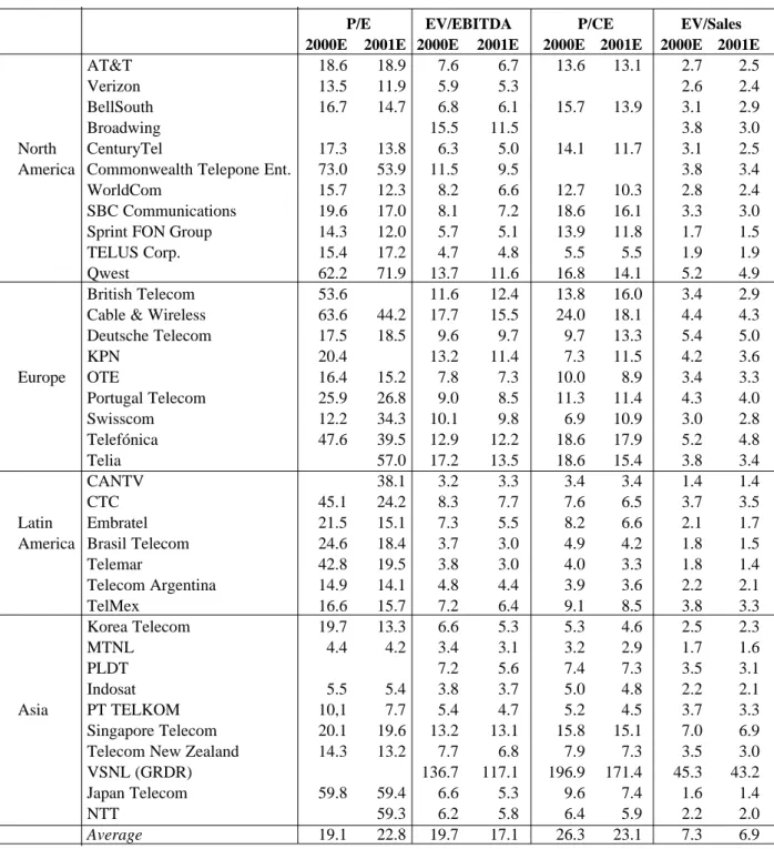
(12) 12. 4.3. Dispersion of the multiples of telecommunications Table 8 shows the leading telecommunications operators divided by geographical area. In the case of North America, Europe, and Latin America, it can be seen that the PER is the multiple with the highest dispersion, particularly for the year 2000E, ranging between 13.5 - 73, 12.2 - 63 and 14.9 - 45.1, respectively. In the case of Asia, the differences are substantial in all multiples, particularly the EV/EBITDA, which ranges between 3.4 and 136.7 (for 2000E) and 3.1 and 117.1 (for 2001E), and the P/CE, with data between 3.2 196.9 and 2.9 - 171.4 for 2000E and 2001E, respectively. Table 9 shows multiples for cellular phone companies. Note, again, the multiples’ wide dispersion. Table 8. Valuation by multiples of telecommunications companies P/E EV/EBITDA 2000E 2001E 2000E 2001E. AT&T Verizon BellSouth Broadwing North CenturyTel America Commonwealth Telepone Ent. WorldCom SBC Communications Sprint FON Group TELUS Corp. Qwest British Telecom Cable & Wireless Deutsche Telecom KPN Europe OTE Portugal Telecom Swisscom Telefónica Telia CANTV CTC Latin Embratel America Brasil Telecom Telemar Telecom Argentina TelMex Korea Telecom MTNL PLDT Indosat Asia PT TELKOM Singapore Telecom Telecom New Zealand VSNL (GRDR) Japan Telecom NTT Average. 18.6 13.5 16.7. 18.9 11.9 14.7. 17.3 73.0 15.7 19.6 14.3 15.4 62.2 53.6 63.6 17.5 20.4 16.4 25.9 12.2 47.6. 13.8 53.9 12.3 17.0 12.0 17.2 71.9 44.2 18.5. 45.1 21.5 24.6 42.8 14.9 16.6 19.7 4.4. 15.2 26.8 34.3 39.5 57.0 38.1 24.2 15.1 18.4 19.5 14.1 15.7 13.3 4.2. 5.5 10,1 20.1 14.3. 5.4 7.7 19.6 13.2. 59.8. 59.4 59.3 22.8. 19.1. 7.6 5.9 6.8 15.5 6.3 11.5 8.2 8.1 5.7 4.7 13.7 11.6 17.7 9.6 13.2 7.8 9.0 10.1 12.9 17.2 3.2 8.3 7.3 3.7 3.8 4.8 7.2 6.6 3.4 7.2 3.8 5.4 13.2 7.7 136.7 6.6 6.2 19.7. Source: Morgan Stanley Dean Witter Research. 15 September 2000.. 6.7 5.3 6.1 11.5 5.0 9.5 6.6 7.2 5.1 4.8 11.6 12.4 15.5 9.7 11.4 7.3 8.5 9.8 12.2 13.5 3.3 7.7 5.5 3.0 3.0 4.4 6.4 5.3 3.1 5.6 3.7 4.7 13.1 6.8 117.1 5.3 5.8 17.1. P/CE 2000E 2001E. 13.6. 13.1. 15.7. 13.9. 14.1. 11.7. 12.7 18.6 13.9 5.5 16.8 13.8 24.0 9.7 7.3 10.0 11.3 6.9 18.6 18.6 3.4 7.6 8.2 4.9 4.0 3.9 9.1 5.3 3.2 7.4 5.0 5.2 15.8 7.9 196.9 9.6 6.4 26.3. 10.3 16.1 11.8 5.5 14.1 16.0 18.1 13.3 11.5 8.9 11.4 10.9 17.9 15.4 3.4 6.5 6.6 4.2 3.3 3.6 8.5 4.6 2.9 7.3 4.8 4.5 15.1 7.3 171.4 7.4 5.9 23.1. EV/Sales 2000E 2001E. 2.7 2.6 3.1 3.8 3.1 3.8 2.8 3.3 1.7 1.9 5.2 3.4 4.4 5.4 4.2 3.4 4.3 3.0 5.2 3.8 1.4 3.7 2.1 1.8 1.8 2.2 3.8 2.5 1.7 3.5 2.2 3.7 7.0 3.5 45.3 1.6 2.2 7.3. 2.5 2.4 2.9 3.0 2.5 3.4 2.4 3.0 1.5 1.9 4.9 2.9 4.3 5.0 3.6 3.3 4.0 2.8 4.8 3.4 1.4 3.5 1.7 1.5 1.4 2.1 3.3 2.3 1.6 3.1 2.1 3.3 6.9 3.0 43.2 1.4 2.0 6.9.

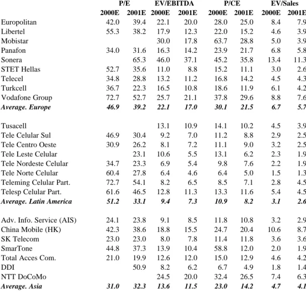
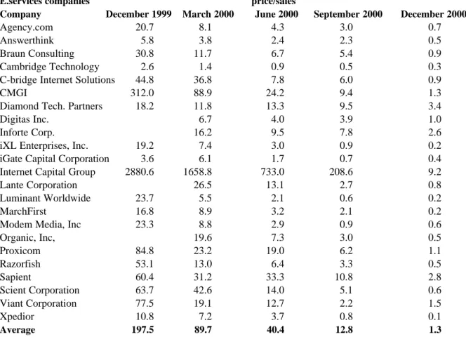
(13) 13. Table 9. Multiples of cellular phone companies. September 2000. P/E EV/EBITDA 2000E 2001E 2000E 2001E. Europolitan Libertel Mobistar Panafon Sonera STET Hellas Telecel Turkcell Vodafone Group. 52.7 34.8 36.7 72.7. 31.6 65.3 35.6 28.8 22.3 52.7. 20.0 12.3 17.8 14.2 37.1 8.8 11.2 10.8 21.1. 28.0 22.0 63.7 23.9 45.2 15.2 16.8 18.6 37.8. 25.0 15.2 28.8 21.7 35.8 11.1 14.2 11.9 29.6. 8.4 4.6 5.0 6.8 13.4 3.0 4.5 6.1 8.8. 7.9 3.9 3.9 5.8 11.3 2.6 4.3 4.2 7.6. 46.9. 39.2. 22.1. 17.0. 30.1. 21.5. 6.7. 5.7. 46.9 30.9 34.7 60.4 72.7 61.6. 30.4 26.2 23.1 23.3 27.8 54.1 46.5. 13.1 9.2 8.1 10.6 6.9 6.4 8.2 12.8. 10.9 7.0 7.2 5.5 5.4 4.6 6.5 11.3. 14.1 11.2 11.1 13.1 9.8 6.4 8.5 13.3. 10.2 8.8 9.0 6.2 7.6 5.0 7.1 11.6. 4.5 2.9 3.2 2.3 2.2 1.5 2.8 5.4. 3.9 2.5 2.5 1.9 1.9 1.3 4.5 4.5. Average. Latin America. 51.2. 33.1. 9.4. 7.3. 10.9. 8.2. 3.1. 2.6. Adv. Info. Service (AIS) China Mobile (HK) SK Telecom SmarTone Total Acces Com. DDI NTT DoCoMo. 24.1 42.3 23.0 44.8 21.0. 23.8 38.6 23.0 37.3 19.9 50.9. 9.1 18.8 8.0 13.9 12.6 8.2 24.5. 8.5 15.5 7.8 10.4 12.0 6.2 20.0. 11.8 24.7 11.4 58.8 15.0 6.7 32.4. 10.8 20.4 11.8 12.0 12.9 4.9 26.5. 3.2 10.6 3.6 2.0 4.6 1.8 7.4. 2.9 8.7 3.6 1.9 4.2 1.4 6.3. Average. Asia. 31.0. 32.3. 13.6. 11.5. 23.0. 14.2. 4.7. 4.1. Tusacell Tele Celular Sul Tele Centro Oeste Tele Leste Celular Tele Nordeste Celular Tele Norte Celular Teleming Celular Part. Telesp Celular Part.. 39.4 38.2. 34.0. EV/Sales 2000E 2001E. 22.1 17.9 30.0 16.3 46.0 11.0 13.2 16.5 25.7. Average. Europe. 42.0 55.3. P/CE 2000E 2001E. 4.4. Dispersion of the multiples of banks Table 10 shows multiples for Spanish and Portuguese banks in November 2000. The PER in 2000 ranges between 10.4 and 30.9; the price to book value multiple ranges between 1.5 and 4.7; the ROE ranges between 12.9% and 28.2%. The multiples are much more homogenous in the case of the Portuguese banks..

(14) 14. Table 10. Multiples of Spanish and Portuguese banks. November 2000. 2000. PER P/BV P/NAV Dividend yield 2001 2002 2000 2001 2000 2000 2001. 21.5 19.6 16.5 30.9 10.4 17.8 13.7 18.6 17.7 13.7 14.0 15.1. 17.3 15.8 14.2 29.9 9.5 16.6 12.4 16.5 16.2 12.2 12.8 13.7. BBVA BSCH Banco Popular Bankinter Banco Pastor Banco Zaragozano Banco Valencia Spain BCP BES BPI Portugal. 13.9 12.9 12.5 27.0 9.2 16.6 11.5 14.8 14.4 11.6 11.4 12.5. 3.9 3.2 4.7 4.0 1.5 1.7 2.2 3.0 3.0 2.6 2.6 2.7. 3.5 2.9 4.1 3.8 1.4 1.6 2.0 2.9 2.8 2.4 2.4 2.5. 3.4 4.2 4.1 3.2 1.5 n.a. 2.2 3.1 3.0 2.6 2.6 2.7. 2.2% 2.6% 3.3% 2.2% 2.8% 2.4% 3.5% 2.7% 2.4% 3.5% 2.9% 2.9%. 2.6% 3.4% 3.9% 2.3% 3.1% 2.9% 5.7% 3.4% 2.6% 4.0% 3.1% 3.3%. ROE 2000 2001. 20.2% 19.6% 28.2% 12.9% 14.7% 15.0% 16.4% 18.1% 18.6% 18.6% 18.6% 18.6%. 21.4% 19.2% 30.7% 12.8% 14.2% 16.0% 17.0% 18.8% 19.8% 14.4% 21.4% 18.5%. ROE/P/BV 2000 2001. 5.2 6.2 6.0 3.2 9.5 8.8 7.4 6.3 6.3 7.3 7.0 6.9. 6.1 6.6 7.5 3.3 10.3 10.0 8.5 6.8 7.0 6.0 8.9 7.3. 4.5. Dispersion of the multiples of Internet companies Table 11 contains the price/sales multiple of Internet companies. Note the wide dispersion and the multiple’s decrease in 2000. Table 11. Multiples of Internet companies in 1999 and 2000 E.services companies Company. December 1999. Agency.com 20.7 Answerthink 5.8 Braun Consulting 30.8 Cambridge Technology 2.6 C-bridge Internet Solutions 44.8 CMGI 312.0 Diamond Tech. Partners 18.2 Digitas Inc. Inforte Corp. iXL Enterprises, Inc. 19.2 iGate Capital Corporation 3.6 Internet Capital Group 2880.6 Lante Corporation Luminant Worldwide 23.7 MarchFirst 16.8 Modem Media, Inc 23.3 Organic, Inc, Proxicom 84.8 Razorfish 53.1 Sapient 60.4 Scient Corporation 63.7 Viant Corporation 77.5 Xpedior 10.8 Average. 197.5. March 2000. price/sales June 2000. September 2000. December 2000. 8.1 3.8 11.7 1.4 36.8 88.9 11.8 6.7 16.2 7.4 6.1 1658.8 26.5 5.5 8.9 8.8 19.6 23.2 13.0 31.2 42.6 19.1 7.2. 4.3 2.4 6.7 0.9 7.8 24.2 13.3 4.0 9.5 3.0 1.7 733.0 13.1 2.1 3.2 2.9 7.3 19.0 6.4 33.3 14.0 12.7 3.7. 3.0 2.3 5.4 0.5 6.0 9.4 9.5 3.9 7.8 0.9 0.7 208.6 2.7 0.6 2.1 0.9 3.0 6.2 3.3 10.8 5.1 2.2 0.8. 0.7 0.5 0.9 0.3 0.9 1.3 3.4 1.0 2.6 0.2 0.4 9.2 0.8 0.2 0.2 0.6 0.5 1.1 0.5 2.8 0.6 1.5 0.1. 89.7. 40.4. 12.8. 1.3.

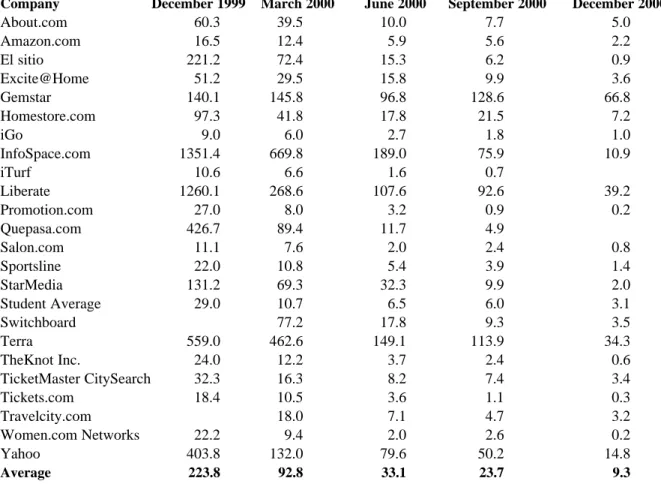
(15) 15. DOT COMS Company. December 1999. About.com Amazon.com El sitio Excite@Home Gemstar Homestore.com iGo InfoSpace.com iTurf Liberate Promotion.com Quepasa.com Salon.com Sportsline StarMedia Student Average Switchboard Terra TheKnot Inc. TicketMaster CitySearch Tickets.com Travelcity.com Women.com Networks Yahoo. 60.3 16.5 221.2 51.2 140.1 97.3 9.0 1351.4 10.6 1260.1 27.0 426.7 11.1 22.0 131.2 29.0. price/sales June 2000. September 2000. 22.2 403.8. 39.5 12.4 72.4 29.5 145.8 41.8 6.0 669.8 6.6 268.6 8.0 89.4 7.6 10.8 69.3 10.7 77.2 462.6 12.2 16.3 10.5 18.0 9.4 132.0. 10.0 5.9 15.3 15.8 96.8 17.8 2.7 189.0 1.6 107.6 3.2 11.7 2.0 5.4 32.3 6.5 17.8 149.1 3.7 8.2 3.6 7.1 2.0 79.6. 7.7 5.6 6.2 9.9 128.6 21.5 1.8 75.9 0.7 92.6 0.9 4.9 2.4 3.9 9.9 6.0 9.3 113.9 2.4 7.4 1.1 4.7 2.6 50.2. 223.8. 92.8. 33.1. 23.7. 559.0 24.0 32.3 18.4. Average. March 2000. December 2000. 5.0 2.2 0.9 3.6 66.8 7.2 1.0 10.9 39.2 0.2 0.8 1.4 2.0 3.1 3.5 34.3 0.6 3.4 0.3 3.2 0.2 14.8 9.3. 5. Volatility of the most widely used parameters for multiples Table 12 shows the average volatility of several of the most commonly used parameters for multiples and of some of the multiples for the 26 largest Spanish companies during the period 1991-99. PER, EBITDA and profit after tax were more volatile than equity value. Table 12. Average volatility of several parameters used for multiples. 26 Spanish companies. 1991-1999. Equity value. Average volatility. 41%. Profit After fax EBITDA. 49%. 59%. Dividends Book value. 20%. 18%. ROE. ROA. PER. 4%. 2%. 76%. 6. Analysts’ recommendations: hardly ever sell Table 13 shows the recommendations of 226 brokers during the period 1989-1994. Note that the recommendations range mostly between hold and buy. Less than 10% of the recommendations are to sell..

(16) 16. Table 14 shows the analysts’ recommendations for Spanish companies in the IBEX 35 index. Note that the recommendations mostly range between holding and buying. Less than 15% of the recommendations are to sell. On 14 February 2000, the IBEX stood at 12,458 points; by 23 October it had fallen to 10,329 points. Table 13. North American analysts’ recommendations. 1989-1994 From ↓. Το → Strong buy. Buy. Hold. Sell. Strong Sell. Sum. Percentage. 8,190 2,323 3,622 115 115. 2,234 4,539 3,510 279 39. 4,012 3,918 13,043 1,826 678. 92 262 1,816 772 345. 154 60 749 375 407. 14,682 11,102 22,740 3,367 1,584. 27.5% 20.8% 42.5% 6.3% 3.0%. 14,365 26.9. 10,601 19.8. 23,477 43.9. 3,287 6.1. 1,745 3.3. 53,475. Strong buy Buy Hold Sell Strong Sell Sum Percentage Source: Welch (2000).. Table 14. Analysts’ recommendations on Spanish stocks (In percentage). Buy. 14 February 2000 Hold. Sell. Buy. 23 October 2000 Hold Sell. ACS Acciona Aceralia Acerinox Acesa Aguas Bna. Alba Altadis Amadeus Bankinter BBVA BSCH Cantábrico Continente Dragados Endesa FCC Ferrovial Gas Natural Iberdrola Indra NH Hoteles Popular Repsol Sogecable Sol Melia Terra Tele pizza Telefónica TPI Unión Fenosa Vallehermoso. 90.0 37.5 82.4 68.8 54.6 69.2 80.0 72.7 75.0 31.6 57.7 63.0 42.9 71.4 50.0 67.9 70.0 50.0 18.8 57.9 55.6 85.0 54.6 75.8 87.5 60.0 87.5 50.0 94.7 50.0 88.2 50.0. 0.0 25.0 5.9 18.8 36.4 15.4 0.0 18.2 0.0 47.4 34.6 37.0 42.9 14.3 41.7 28.6 30.0 30.0 43.8 36.8 33.3 15.0 36.4 18.2 0.0 26.7 0.0 37.5 5.3 37.5 11.8 10.0. 10.0 37.5 11.8 12.5 9.1 15.4 20.0 9.1 25.0 21.1 7.7 0.0 14.3 14.3 8.3 3.6 0.0 20.0 37.5 5.3 11.1 0.0 9.1 6.1 12.5 13.3 12.5 14.3 0.0 18.5 0.0 40.0. 81.8 88.9 79.0 70.6 72.7 50.0 62.5 76.9 58.6 33.3 54.7 51.8 27.8 53.3 66.7 52.9 51.3 70.0 22.2 50.0 76.9 81.3 70.0 48.6 62.4 76.5 59.1 41.5 86.3 38.5 85.7 76.9. 18.2 0.0 21.1 17.7 27.3 36.7 25.0 15.4 34.3 38.9 33.5 48.2 44.4 40.0 33.3 44.4 48.7 30.0 50.0 38.0 23.1 18.8 30.0 45.9 25.9 17.7 31.8 35.4 11.8 30.8 14.3 23.1. 0.0 11.1 0.0 11.8 0.0 13.1 12.5 7.7 7.1 27.8 11.8 0.0 27.8 6.7 0.0 2.8 0.0 0.0 27.8 12.0 0.0 0.0 0.0 5.6 11.8 5.9 9.1 23.1 2.0 30.8 0.0 0.0. Average. 64.1. 23.1. 13.1. 61.8. 29.8. 8.4. Source: Actualidad Económica..

(17) 17. Key concepts Multiple Dispersion Analysts’ recommendations. References Fernández, Pablo (2001), “Internet Valuations: The Case of Terra-Lycos” SSRN Working Paper. http://papers.ssrn.com/sol3/papers.cfm?abstract_id=265608 Moody’s Investors Service (June 2000), Putting EBITDA In Perspective. Morgan Stanley Dean Witters, How We Value Stocks, 15 September 1999. Welch, Ivo (2000), “Herding among Security Analysts”, Journal of Financial Economics, 58, pp. 369-396..

(18)

No results found