Evaluating Combined Non-Replicable Forecasts

Full text

(1)KIER DISCUSSION PAPER SERIES KYOTO INSTITUTE OF ECONOMIC RESEARCH Discussion Paper No.744. “Evaluating Combined Non-Replicable Forecasts”. Michael McAleer. December 2010. KYOTO UNIVERSITY KYOTO, JAPAN.

(2) Evaluating Combined Non-Replicable Forecasts*. Chia-Lin Chang Department of Applied Economics National Chung Hsing University Taichung, Taiwan. Philip Hans Franses Econometric Institute Erasmus School of Economics Erasmus University Rotterdam The Netherlands. Michael McAleer Econometric Institute Erasmus School of Economics Erasmus University Rotterdam The Netherlands and Tinbergen Institute Amsterdam, The Netherlands and Institute of Economic Research Kyoto University, Japan. Revised: December 2010. * For financial support, the first author wishes to thank the National Science Council, Taiwan, and the third author wishes to thank the Australian Research Council, National Science Council, Taiwan, and the Japan Society for the Promotion of Science.. 1.

(3) Abstract. Macroeconomic forecasts are often based on the interaction between econometric models and experts. A forecast that is based only on an econometric model is replicable and may be unbiased, whereas a forecast that is not based only on an econometric model, but also incorporates an expert’s touch, is non-replicable and is typically biased. In this paper we propose a methodology to analyze the qualities of combined non-replicable forecasts. One part of the methodology seeks to retrieve a replicable component from the non-replicable forecasts, and compares this component against the actual data. A second part modifies the estimation routine due to the assumption that the difference between a replicable and a non-replicable forecast involves a measurement error. An empirical example to forecast economic fundamentals for Taiwan shows the relevance of the methodological approach.. Key words: Combined forecasts, efficient estimation, generated regressors, replicable forecasts, non-replicable forecasts, expert’s intuition. JEL Classifications: C53, C22, E27, E37. 2.

(4) 1. Introduction. Econometric models are frequently used to provide base-level forecasts in macroeconomics. Usually, these model-based forecasts are adjusted by experts who have domain knowledge. For example, Franses, Kranendonk and Lanser (2010) document that this holds for all forecasts (for GDP, inflation, and so on) generated from the large macroeconomic model created at the CPB Netherlands Bureau for Economic Policy Analysis. The difference between the pure model-based forecast and the final forecast is often called intuition or judgment. It is a trade secret owned by a forecaster, as it is rarely written down, but it can have significant value in forecasting key economic fundamentals.. A forecast that is based on an econometric model is replicable and may be unbiased, whereas a forecast that is not based on an econometric model is non-replicable and is typically biased. In practice, most macroeconomic forecasts (from CPB, but also from the FED, the World Bank, OECD and IMF) are non-replicable. In some cases, the model-based forecasts are available and one can then derive their link with the final expert-touched forecasts, but in many cases only the final forecast is available.. In this paper we examine the evaluation of the quality of a range of available non-replicable forecasts, with a specific focus on the combinations of these potentially biased forecasts. For this, we propose a methodology that approaches this issue from two different angles. The first aims to de-bias the non-replicable forecast by retrieving and comparing their replicable components. The second approach modifies the estimation method.. In order to illustrate, we use data from Taiwan for three reasons. First, a consistent data set is available for the government and two professional quarterly forecasts of economic fundamentals over an extended period. Second, no previous comparison seems to have been made of the competing combined forecasts. Third, there does not seem to have been any comparison of individual and combined forecasts based on an optimal subset of the multiple forecasts.. The plan of the remainder of the paper is a follows. Section 2 presents the econometric model specification, analyses replicable and non-replicable forecasts, considers optimal forecasts and efficient estimation methods, compares individual replicable forecasts with an optimal subset combined replicable forecast, and presents a direct test of forecasting expertise. The data analysis 3.

(5) and a relevant empirical example of multiple forecasts of economic fundamentals for Taiwan are discussed in Section 3. Some concluding comments are given in Section 4.. 2. Model Specification. In this section we present a method to evaluate non-replicable forecasts. First we deal with individual forecasts, and then we consider combined forecasts.. 2.1. Individual Forecasts. Consider a variable y as a T x 1 vector of observations to be explained (typically, an economic fundamental, such as the inflation rate or the real GDP growth rate), and assume that there are m forecasts X i for this variable y, where i = 1,2,…,m. In order to evaluate the quality of each individual forecast, one can consider the auxiliary regression y = α i + β i X i + ui. (1). where the error term has mean zero and common variance σ u2i . The interest lies in the estimated values of α i and β i , where the true parameters are 0 and 1, respectively.. When the forecasts, X i , would be fully based on an econometric model, then one can apply ordinary least squares (OLS) to (1) to estimate the parameters, α i and β i , and test their values against 0 and 1, respectively. However, when X i is the end-product of the interaction between model output and an expert’s touch, OLS is not valid (see Franses et al. (2009)).. There are now two possible strategies to approach this issue. The first is to replace the X i by a model-based forecast created by the analyst. Assume that this analyst has access to publicly available information contained in the T x k i matrix Wi . The analyst can now run the regression X i = Wi δ i + η i. (2). 4.

(6) where it is assumed that the first column of Wi concerns the intercept, and where the error term has mean zero and common variance σ η2i . Applying OLS to (2) yields X̂ i . In a next step, the analyst can replace (1) by. y = α i + β i Xˆ i + ui. (3). As the regressor X̂ i in (3) is a generated regressor, the error term in (3) also contains a term with the measurement error η i in (2), and hence when OLS is used, it is essential that the appropriate covariance matrix is computed. Franses et al. (2009) show how to do this. An alternative is to apply OLS to (3) and to incorporate the Newey-West HAC covariance matrix estimator.. A second approach is to replace (1) by y = α i + β i (Wi δ i + η i ) + u i. (4). which can be written as y = α i + β i X i + u i − β iη i. (5). for which it is clear that OLS is inconsistent for (5) as X i is correlated with η i . A simple solution is to use the Generalized Methods of Moments (GMM).. 2.2. Combined Forecasts. An alternative to evaluating the m forecasts individually is to combine them into a combined forecast. m. ∑λ X i =1. i. (6). i. where λi are known constants. Typical constants would be λi = possible. The equivalent of (1) now becomes 5. 1 m. , but also other variants are.

(7) m. y = α + β ∑ λi X i + u. (7). i =1. where the error term has mean zero and common variance σ u2 .. The equivalent of (3) now becomes. m. y = α + β ∑ λi Xˆ i + ε. (8). i =1. with. m. ε = u + β ∑ λi ( X i − Xˆ i ). (9). i =1. Given (2), we have. Xˆ i = Wi (Wi 'Wi ) −1Wi ' X i = Pi X i. (10). Substituting (10) into (9) gives. m. ε = u + β ∑ λi (Wi δ i − Pi X i ) i =1. or equivalently. m. ε = u − β ∑ λi Piη i. (11). i =1. The covariance matrix of ε is given by. 6.

(8) m. V = E (εε ' ) = σ u2 I + β 2 ∑ λi2σ i2 Pi. (12). i =1. if u and η i are uncorrelated for all i = 1,2,..., m. If OLS is used to estimate (8), the covariance matrix should be based on (12).. Defining. m. H = [1; ∑ λi Xˆ i ]. (13). i ==1. and. θ ' = (α , β ). then (8) can be written as y = Hθ + ε. (14). so that the covariance matrix of θˆ is given by Var (θˆ) = ( H ' H ) −1 H 'VH ( H ' H ) −1. (15). When V in (12) is substituted in (15), one has ⎛ m ⎞ Var (θˆ) = σ u2 ( H ' H ) −1 + β 2 ( H ' H ) −1 H ' ⎜ ∑ λiσ i2 Pi ⎟ H ( H ' H ) −1 ⎝ i =1 ⎠. (16). which shows that the standard OLS covariance matrix of θˆ , namely the first term on the right-hand side of (16), leads to a downward bias in the covariance matrix and a corresponding upward bias in the corresponding t-ratios. The covariance matrix in (16) can be consistently estimated by the Newey-West HAC covariance matrix. Smith and McAleer (1994) evaluate the finite sample. 7.

(9) properties of the HAC estimator for purposes of testing hypotheses and constructing confidence intervals in the case of generated regressors.. Again, an alternative approach builds on (5) and is given as. m. y = α + β ∑ λi ( X i − η i ) + u i =1. or. m m ⎛ ⎞ y = α + β ∑ λi X i + ⎜ u − β ∑ λiη i ⎟ i =1 i =1 ⎝ ⎠. m. As. ∑λ X i =1. i. (17). m. i. is correlated with. ∑λη i =1. i. i. , one again needs to apply GMM.. 3. Data and Empirical Analysis. Since 1978, actual data and three sets of updated forecasts of the inflation rate and real GDP growth rate have been released by the Government of Taiwan, Republic of China (for further details, see Chang et al. (2009)). The unemployment rate is not regarded as a key economic fundamental in Taiwan. In this paper, we use the most recent revised government forecasts. The government forecasts (F1) and actual values of the inflation rate and real GDP growth rate are obtained from the Quarterly National Economic Trends, Directorate-General of Budget, Accounting and Statistics, Executive Yuan, Taiwan, 1980-2009. The forecasts from the two private forecasting institutions are obtained from the Chung-Hua Institution for Economic Research (F2) and Taiwan Institute of Economic Research (F3). In addition to comparing actual data on both the inflation rate and real growth rate with three sets of forecasts, four combined forecasts are also considered, namely the mean of all three forecasts and of three pairs of mean forecasts. In the Tables, M refers to the mean of all three forecasts, M12 refers to the mean of F1 and F2, M13 refers to the mean of F1 and F3, and M23 refers to the mean of F2 and F3. 8.

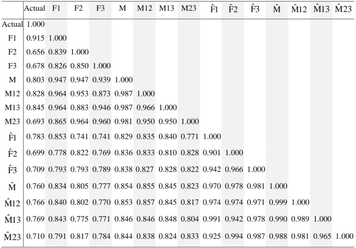
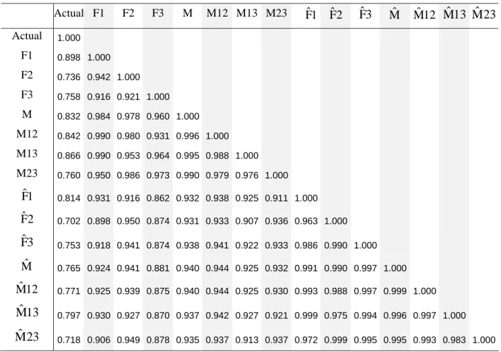
(10) As the actual values of the inflation rate and real GDP growth rate are available, the accuracy of the government and two private forecasts, as well as the effects of econometric model versus intuition, can be compared and tested. The sample period used for the actual values and the three sets of forecasts of seasonally unadjusted quarterly inflation rate and real growth rate of GDP is 1995Q32009Q2, for a total of 56 observations.. We have analyzed the data on unit roots and structural breaks. The diagnostics for unit roots (which are unreported) indicate that we can work with the growth rates data, as in Figures 1 and 2. Visual inspection from the same graphs does not suggest potential structural breaks, and there is also no evidence of structural breaks caused by any changes in measurement methods at the government agency and two private forecasting institutions in Taiwan.. The inflation rate and the three forecasts, F1, F2 and F3, are given in Figure 1, and the corresponding plots of the real GDP growth rate and the three forecasts are given in Figure 2. Figure 3 gives the inflation rate, the mean of the three forecasts, and the means of pairs of forecasts, while the corresponding plots of the real GDP growth rate, the mean of the three forecasts, and the means of pairs of forecasts are given in Figure 4.. Table 1 gives the correlations of the inflation rate, three forecasts, the mean of three forecasts, the means of pairs of forecasts (and their replicable counterparts, which are obtained from Tables 4 and 5 (to be discussed below) , with the corresponding plots of the real GDP growth rate given in Table 2. In these two tables, hats (circumflex) denote their replicable counterparts. In Tables 1 and 2, the highest correlations for both the actual inflation rate and the real GDP growth rate are with F1, followed by M13; for both variables, F1 is highly correlated with M12, M13 and M23, F2 is highly correlated with M12 and M23, F3 is highly correlated with M23, M is highly correlated with M12 and M13, M12 is highly correlated with M13, and M13 is highly correlated with M23. The correlations are generally higher between the original variables than between their fitted counterparts.. The goodness-of-fit measures, namely root mean square error (RMSE) and mean absolute deviation (MAD), of the replicable and non-replicable forecasts are given in Table 3 for both variables. For the non-replicable forecasts, in the upper panel of Table 3, the single forecast, F1, is best for both variables using RMSE and MAD, while the mean of two forecasts, M13, is second best for the 9.

(11) inflation rate, and M12 is second best for the real GDP growth rate. A similar outcome holds for the replicable forecasts, with F̂1 best for both variables using RMSE and MAD, while M̂13 is second best for both variables using RMSE and MAD.. These results suggest that, in general, the first single forecast is best in terms of both RMSE and MAD, followed by a mean combination of the first and third forecasts, for both the inflation rate and real GDP growth rate, regardless of whether a non-replicable or replicable forecast is used. Table 3 also shows that the biased non-replicable forecasts are apparently much more accurate than the replicable forecasts. Hence, the added intuition of the experts seems to lead to substantial improvement. This improvement is most evident for F1, where RMSE for the replicable forecast is about twice as large as for the non-replicable forecast.. In Tables 4a-4b and Tables 5a-5b, we report on the retrieval of a replicable part from the nonreplicable forecasts based on public information for the inflation rate and real GDP growth rate, respectively. This public information is set at one-period lagged real growth, one-period lagged inflation, one period lagged forecast for forecaster 1, one period lagged forecast for forecaster 2 and one period lagged forecast for forecaster 3.. It is evident that the lagged values of the forecasts of all three forecasters are insignificant in all four tables, so the forecasters do not seem to include each other’s predictions. The one-period lagged real GDP growth rate is significant for all seven forecasts for both the inflation rate and real GDP growth rate. Apart from the significant case of F1 in Table 4a, the one-period lagged inflation rate is not significant in capturing expertise for any of the seven forecasts for either variable. The F tests for the significance of the replicable part in Tables 4a-4b and Tables 5a-5b indicate clearly that the expertise in equation (3) is captured by the one-period lagged variables, specifically the one-period lagged real GDP growth rate.. In order to examine if the replicable forecasts are unbiased, we consider equations (3) and (8) for three forecasts and four mean forecasts, which are given in Tables 6a-6b for the inflation rate and real GDP growth rate. As the replicable forecasts lead to generated regressors, the appropriate Newey-West HAC standard errors are calculated for valid inference. The F test is a test of the null hypothesis H 0 : α = 0 , β i = 1 for i = 1,2,3. If the null hypothesis is not rejected, then the model via the replicable forecast can predict the actual value, whereas rejection of the null means that expert 10.

(12) intuition could triumph over the model in case the non-replicable forecasts are not biased. Except for F1 and F2 for the real GDP growth rate in Table 6a, the null hypothesis is rejected in all cases, which makes it clear that intuition is significant in explaining actual values, and hence dominates the model. This supports the RMSE and MAD scores in Table 3.. Tables 7a-7b and Tables 8a-8b focus on the accuracy of the non-replicable forecasts for three forecasts and four mean forecasts in equations (5) and (17) for the inflation rate and real GDP growth rate. As the non-replicable forecasts are correlated with the measurement errors, GMM is necessary for valid inference, where the instrument list for GMM for forecaster i includes oneperiod lagged real growth, one-period lagged inflation, one-period lagged forecast for forecaster 1, and one-period lagged forecast for forecaster 2 and one period lagged forecast for forecaster 3. The F test is a test of the null hypothesis H 0 : α = 0 , β i = 1 for i = 1,2,3. Conditional on the information set, if the null hypothesis is not rejected, then the non-replicable forecast can accurately predict the actual value, whereas rejection of the null hypothesis means that the non-replicable forecast is biased.. Except in one case, namely GMM estimation of M for the inflation rate in Table 7b, the null hypothesis is rejected for all individual forecasts and mean forecasts. Thus, conditional on the information set, the non-replicable forecast cannot predict the actual inflation rate. Ignoring the OLS results in Tables 8a-8b, mirroring the results in Tables 7a-7b, except for one case, namely GMM estimation of F1 for the real GDP growth rate in Table 8a, the null hypothesis is rejected for all individual forecasts and mean forecasts. Thus, conditional on the information set, the nonreplicable forecast cannot predict the actual real GDP growth rate. If we compare the F test values in Tables 7 and 8 with those in Table 6, we see that the non-replicable forecasts have greater bias than the replicable forecasts. Again, the non-replicable forecasts are much more accurate than the replicable forecasts, which means that the intuition possessed by the forecasters greatly improves any model-based forecasts. As in many other studies, combining forecasts can be beneficial. For inflation, we see that the GMM-based results in Table 7b indicate the M delivers unbiased forecasts. For GDP growth, the situation is somewhat different. There we see that the non-replicable F1 is unbiased (Table 8a), and Table 3 also suggests it has the smallest forecast error. However, Table 8b clearly shows that combining forecasts is not sensible as all the combinations examined in Table 8b lead to biased forecasts.. 11.

(13) 4. Concluding Remarks. A forecast that is based on an econometric model is replicable and may be unbiased, whereas a forecast that is not based on an econometric model is non-replicable and is typically biased. Government and professional forecasters alike can, and do, provide both replicable and nonreplicable forecasts. Both types of forecasts can be combined into a single combined forecast, such as a mean or trimmed mean forecast.. This paper developed a methodology to evaluate combined forecasts using efficient estimation methods, and compared individual replicable forecasts with combined forecasts. An empirical example to forecast economic fundamentals for Taiwan showed the relevance of the methodological approach proposed in the paper. The empirical analysis showed that replicable and non-replicable forecasts could be distinctly different from each other, that efficient and inefficient estimation methods, as well as consistent and inconsistent covariance matrix estimates, could lead to significantly different outcomes, combined forecasts could yield different forecasts from their multiple individual components, and the relative importance of econometric model versus intuition could be evaluated in terms of forecasting performance.. It was shown that individual forecasts could perform quite differently from the mean forecasts of two or three individual forecasts, that intuition was significant in explaining actual values, and hence dominated the model, and that expert intuition that has been used to obtain the non-replicable forecasts of the inflation rate and real GDP growth rate was not sufficient to forecast accurately the actual values.. One of the major findings is that a proper analysis of combined forecasts could suggest a weaker dominance of other forecasts, as is typically documented in the literature. The GMM-based analysis shows that the combined forecasts could well be found to be biased, while the OLS-based analysis did not give any such warning signals.. 12.

(14) References. Chang, C.-L., P.H. Franses and M. McAleer (2009), How accurate are government forecasts of economic fundamentals? The case of Taiwan, International Journal of Forecasting, to appear. Available at SSRN: http://ssrn.com/abstract=1431007. Franses, P.H., H. Kranendonk, and D. Lanser (2010), One model and various experts: Evaluating Dutch macroeconomic forecasts, International Journal of Forecasting, to appear. Franses, P.H., M. McAleer and R. Legerstee (2009), Expert opinion versus expertise in forecasting, Statistica Neerlandica, 63, 334-346. Smith, J. and M. McAleer (1994), Newey-West covariance matrix estimates for models with generated regressors, Applied Economics, 26, 635-640.. 13.

(15) Figure 1. Inflation Rate and Three Forecasts, 1995Q3-2009Q2. 5 4 3 2 1 0 -1 -2 1996. 1998. 2000 Actual. 2002 F1. 2004 F2. 2006. 2008. F3. Figure 2. Real GDP Growth Rate and Three Forecasts, 1995Q3-2009Q2. 10.0 7.5 5.0 2.5 0.0 -2.5 -5.0 -7.5 -10.0 1996. 1998. 2000 Actual. 2002 F1. 14. 2004 F2. 2006 F3. 2008.

(16) Figure 3. Inflation Rate, Mean of Three Forecasts, Means of Pairs of Forecasts, 1995Q3-2009Q2. 5. 4. 3. 2. 1. 0. -1 1996. 1998. 2000. 2002. Actual M13. 2004. M M23. 2006. 2008. M12. Figure 4. Real GDP Growth Rate, Mean of Three Forecasts, Means of Pairs of Forecasts, 1995Q3-2009Q2. 10.0 7.5 5.0 2.5 0.0 -2.5 -5.0 -7.5 -10.0 1996. 1998. 2000. 2002. Actual M13. M M23. 15. 2004. 2006 M12. 2008.

(17) Table 1. Correlations of Inflation Rate, Three Forecasts, Mean of Three Forecasts, Means of Pairs of Forecasts, and their Replicable Counterparts Actual F1. F2. F3. M. M12 M13 M23. F̂1. F̂2. F̂3. M̂. M̂12 M̂13 M̂23. Actual 1.000 F1. 0.915 1.000. F2. 0.656 0.839 1.000. F3. 0.678 0.826 0.850 1.000. M. 0.803 0.947 0.947 0.939 1.000. M12 0.828 0.964 0.953 0.873 0.987 1.000 M13 0.845 0.964 0.883 0.946 0.987 0.966 1.000 M23 0.693 0.865 0.964 0.960 0.981 0.950 0.950 1.000. F̂1. 0.783 0.853 0.741 0.741 0.829 0.835 0.840 0.771 1.000. F̂2. 0.699 0.778 0.822 0.769 0.836 0.833 0.810 0.828 0.901 1.000. F̂3. 0.709 0.793 0.793 0.789 0.838 0.827 0.828 0.822 0.942 0.966 1.000. M̂. 0.760 0.834 0.805 0.777 0.854 0.855 0.845 0.823 0.970 0.978 0.981 1.000. M̂12 0.766 0.840 0.802 0.770 0.853 0.857 0.845 0.817 0.974 0.974 0.971 0.999 1.000. M̂13 0.769 0.843 0.775 0.771 0.846 0.846 0.848 0.804 0.991 0.942 0.978 0.990 0.989 1.000 M̂23 0.710 0.791 0.817 0.784 0.844 0.838 0.824 0.833 0.925 0.994 0.987 0.988 0.981 0.965 1.000 Notes: F1: DGBAS: Directorate General of Budget, Accounting and Statistics (Government), F2: ChungHua: Chung-Hua Institution for Economic Research, F3: Taiwan: Taiwan Institute of Economic Research, M: Mean of three forecasts, M12: Mean of F1 and F2, M13: Mean of F1 and F3, M23: Mean of F2 and F3. Hats (circumflex) denote the replicable counterparts.. 16.

(18) Table 2. Correlations of Real GDP Growth Rate, Three Forecasts, Mean of Three Forecasts, Means of Pairs of Forecasts, and their Replicable Counterparts Actual F1 Actual. F2. F3. M. M12 M13 M23. F̂1. F̂2. F̂3. M̂. M̂12 M̂13 M̂23. 1.000. F1. 0.898 1.000. F2. 0.736 0.942 1.000. F3. 0.758 0.916 0.921 1.000. M. 0.832 0.984 0.978 0.960 1.000. M12. 0.842 0.990 0.980 0.931 0.996 1.000. M13. 0.866 0.990 0.953 0.964 0.995 0.988 1.000. M23. 0.760 0.950 0.986 0.973 0.990 0.979 0.976 1.000. F̂1. 0.814 0.931 0.916 0.862 0.932 0.938 0.925 0.911 1.000. F̂2. 0.702 0.898 0.950 0.874 0.931 0.933 0.907 0.936 0.963 1.000. F̂3. 0.753 0.918 0.941 0.874 0.938 0.941 0.922 0.933 0.986 0.990 1.000. M̂. 0.765 0.924 0.941 0.881 0.940 0.944 0.925 0.932 0.991 0.990 0.997 1.000. M̂12. 0.771 0.925 0.939 0.875 0.940 0.944 0.925 0.930 0.993 0.988 0.997 0.999 1.000. M̂13. 0.797 0.930 0.927 0.870 0.937 0.942 0.927 0.921 0.999 0.975 0.994 0.996 0.997 1.000. M̂23. 0.718 0.906 0.949 0.878 0.935 0.937 0.913 0.937 0.972 0.999 0.995 0.995 0.993 0.983 1.000. Notes: F1: DGBAS: Directorate General of Budget, Accounting and Statistics (Government), F2: ChungHua: Chung-Hua Institution for Economic Research, F3: Taiwan: Taiwan Institute of Economic Research, M: Mean of three forecasts, M12: Mean of F1 and F2, M13: Mean of F1 and F3, M23: Mean of F2 and F3. Hats (circumflex) denote the replicable counterparts.. 17.

(19) Table 3 Goodness-of-fit of Replicable and Non-Replicable Forecasts for Three Forecasts, Means of Three Forecasts, Means of Pairs of Forecasts, 1995Q3-2009Q2. Inflation Rate. Real GDP Growth Rate. Non-replicable Forecasts. RMSE. MAD. RMSE. MAD. F1. 0.413. 0.524. 3.795. 1.323. F2. 1.409. 0.943. 8.079. 1.888. F3. 1.082. 0.758. 9.919. 2.123. M. 0.856. 0.726. 7.433. 1.865. M12. 0.790. 0.715. 5.568. 1.584. M13. 0.627. 0.619. 6.383. 1.744. M23. 1.201. 0.836. 9.690. 2.130. Inflation Rate. Real GDP Growth Rate. Replicable Forecasts. RMSE. MAD. RMSE. MAD. F̂1. 0.895. 0.754. 6.209. 1.946. F̂2. 1.325. 0.964. 9.678. 2.262. F̂3. 1.108. 0.851. 10.51. 2.217. M̂. 1.064. 0.841. 8.364. 2.112. M̂12. 1.061. 0.838. 7.691. 2.082. M̂13. 0.946. 0.777. 7.666. 2.020. M̂23. 1.222. 0.917. 10.01. 2.245. Note: RMSE and MAD denote root mean square error and mean absolute deviation, respectively.. 18.

(20) Table 4a Retrieving Replicable Components from the three Non-Replicable Forecasts Included Variables. Inflation Rate F1. F2. F3. 0.092. 0.401. 0.176. (0.235). (0.243). (0.246). 0.127. 0.156. 0.103. (0.030)***. (0.030)***. (0.031)***. 0.544. 0.133. 0.119. (0.228)**. (0.225). (0.240). 0.040. 0.266. 0.255. (0.368). (0.373). (0.383). -0.155. 0.167. 0.175. (0.263). (0.261). (0.274). 0.312. -0.079. 0.072. (0.224). (0.213). (0.240). 0.684. 0.620. 0.538. 17.89***. 12.08***. 9.840***. Intercept. Real GDP Growth(t-1). Inflation(t-1). F1(t-1). F 2(t-1). F 3(t-1). Adj. R2 F test. Notes: The regression model is (2) where i = 1 for F1 forecast (government), i = 2 for F2 forecast (ChungHwa institution), and i = 3 for F3 forecast (Taiwan institution). Wi in (2) for the forecast for forecaster 1 is approximated by one-period lagged real growth, one-period lagged inflation, one period lagged forecast for forecaster 1, one period lagged forecast for forecaster 2 and one period lagged forecast for forecaster 3. The F test is a test of expertise. Standard errors in parentheses. ** and *** denote significance at the 5% and 1% levels, respectively.. 19.

(21) Table 4b Retrieving Replicable Components from the Four Non-Replicable Mean Forecasts Included Variables. Inflation Rate M. M12. M13. M23. 0.304. 0.291. 0.153. 0.347. (0.221). (0.229). (0.218). (0.226). 0.135. 0.149. 0.116. 0.130. (0.027)***. (0.029)***. (0.028)***. (0.028)***. 0.274. 0.312. 0.353. 0.146. (0.204). (0.211). (0.212). (0.209). 0.222. 0.214. 0.152. 0.237. (0.337). (0.351). (0.339). (0.345). 0.034. -0.040. 0.002. 0.190. (0.236). (0.246). (0.242). (0.242). 0.035. 0.090. 0.157. -0.032. (0.198). (0.200). (0.212). (0.203). 0.682. 0.682. 0.665. 0.639. 15.15***. 15.55***. 16.12***. 12.68***. Intercept. Real GDP Growth(t-1). Inflation(t-1). F1(t-1). F 2(t-1). F 3(t-1). Adj. R2 F test. Notes: The regression model is (2) where i = 1 for mean of 3 forecasters, i = 2 for mean of F1 and F2, i = 3 for mean of F1 and F3, and i = 4 for mean of F2 and F3. Wi in (2) for the forecast for forecaster 1 is approximated by one-period lagged real growth, one-period lagged inflation, one period lagged forecast for forecaster 1, one period lagged forecast for forecaster 2 and one period lagged forecast for forecaster 3. The F test is a test of expertise. Standard errors in parentheses. *** denotes significance at the 1% level.. 20.

(22) Table 5a Retrieving Replicable Components from the Three Non-Replicable Forecasts Included Variables. Real GDP Growth Rate F1. F2. F3. 0.495. 0.765. 2.077. (0.761). (0.502). (0.546)***. 0.664. 0.246. 0.222. (0.141)***. (0.095)**. (0.102)**. -0.172. -0.093. -0.035. (0.160). (0.108). (0.116). 0.131. 0.383. 0.220. (0.382). (0.256). (0.275). 0.407. 0.577. 0.126. (0.446). (0.307)*. (0.321). -0.344. -0.400. -0.069. (0.386). (0.259). (0.277). 0.844. 0.885. 0.725. 45.52***. 59.74***. 22.05***. Intercept. Real GDP Growth(t-1). Inflation(t-1). F1(t-1). F2(t-1). F3(t-1). Adj. R2 F test. Notes: The regression model is (2) where i = 1 for F1 forecast (government), i = 2 for F2 forecast (ChungHwa institution), and i = 3 for F3 forecast (Taiwan institution). Wi in (2) for the forecast for forecaster i is approximated by one-period lagged real growth, one-period lagged inflation, one period lagged forecast for forecaster 1, one period lagged forecast for forecaster 2 and one period lagged forecast for forecaster 3. The F test is a test of expertise. Standard errors in parentheses. * , ** and *** denote significance at the 10%, 5% and 1% levels, respectively.. 21.

(23) Table 5b Retrieving Replicable Components from the Four Non-Replicable Mean Forecasts Included Variables. Real GDP Growth Rate M3. M12. M13. M23. 1.053. 0.577. 1.283. 1.391. (0.554)*. (0.613). (0.597)**. (0.477)***. 0.392. 0.471. 0.447. 0.235. (0.106)***. (0.116)***. (0.111)***. (0.091)**. -0.072. -0.110. -0.099. -0.050. (0.120). (0.132). (0.127). (0.103). 0.200. 0.212. 0.168. 0.291. (0.284). (0.313). (0.301). (0.244). 0.461. 0.569. 0.272. 0.402. (0.339). (0.374). (0.351). (0.292). -0.331. -0.418. -0.210. -0.271. (0.286). (0.315). (0.303). (0.246). 0.865. 0.875. 0.834. 0.859. 48.55***. 53.98***. 41.21***. 46.10***. Intercept. Real GDP Growth(t-1). Inflation(t-1). F1(t-1). F2(t-1). F3(t-1). Adj. R2 F test. Notes: The regression model is (2) where i = 1 for mean of 3 forecasters, i = 2 for mean of F1 and F2, i = 3 for mean of F1 and F3, and i = 4 for mean of F2 and F3. Wi in (2) for the forecast for forecaster i is approximated by one-period lagged real growth, one-period lagged inflation, one period lagged forecast for forecaster 1, one period lagged forecast for forecaster 2 and one period lagged forecast for forecaster 3. The F test is a test of expertise. Standard errors in parentheses. *, ** and *** denote significance at the 10%, 5% and 1% levels, respectively.. 22.

(24) Table 6a Are Replicable Forecasts for Three Forecasts Accurate?. Estimation Method OLS HAC OLS HAC OLS HAC. Estimation Method OLS HAC OLS HAC OLS HAC. Inflation Rate Intercept. F1. -0.340 (0.248) [0.156]***. 1.035 (0.135)*** [0.115]***. -0.729 (0.358)** [0.305]***. F2. F3. 1.126 (0.185)** [0.180]***. -0.673 (0.328)** [0.237]***. 1.249 (0.191)*** [0.176]***. Adj. R2. F Test. 0.598. 3.58**. 0.493. 6.17***. 0.517. 5.03**. Real GDP Growth Rate Intercept. F1. -0.374 (0.591) [0.710]. 1.081 (0.127) [0.128]***. -1.107 (0.909) [1.094]. F2. F3. 1.220 (0.209)*** [0.209]***. -4.396 (1.216)*** [1.434]***. 1.982 (0.288)*** [0.296]***. Adj. R2. F Test. 0.637. 0.20. 0.447. 0.56. 0.531. 5.63***. Notes: The regression model is (3) where i = 1 for F1 forecast (government), i = 2 for F2 forecast (ChungHwa institution), and i = 3 for F3 forecast (Taiwan institution). Standard errors in parentheses. Newey-West HAC standard errors are in brackets. ** and *** denote significance at the 5% and 1% levels, respectively. The F test is a test of the null hypothesis H 0 : α = 0 , β i = 1 , i = 1,2,3.. 23.

(25) Table 6b Are Replicable Forecasts for Four Combined Forecasts Accurate? Inflation Rate. Estimation Method. OLS HAC OLS HAC OLS HAC OLS HAC Estimation Method. OLS HAC OLS HAC OLS HAC OLS HAC. Intercept. M. -0.693 (0.306)** [0.264]**. 1.195 (0.167)*** [0.179]***. -0.632 (0.295)** [0.257]**. M12. M13. M23. 1.134 (0.157)*** [0.167]***. -0.534 (0.276)* [0.190]***. 1.171 (0.157)*** [0.145]***. -0.788 (0.351)** [0.325]**. 1.216 (0.190)*** [0.225]***. Adj. R2. F Test. 0.562. 4.55**. 0.568. 4.38**. 0.583. 4.39**. 0.505. 4.50**. Adj. R2. F Test. 0.548. 1.93. 0.559. 0.65. 0.605. 2.30*. 0.472. 2.47*. Real GDP Growth Rate Intercept. M. -1.576 (0.823)* [1.215]. 1.353 (0.190)*** [0.208]***. -0.784 (0.719) [1.074]. M12. M13. M23. 1.172 (0.161)*** [0.176]***. -1.830 (0.771)** [1.100]. 1.412 (0.177)*** [0.186]***. -2.314 (1.043)** [1.572]. 1.500 (0.244)*** [0.286]***. Notes: The regression model is (8) where i = 1 for mean of 3 forecasters, i = 2 for mean of F1 and F2, i = 3 for mean of F1 and F3, and i = 4 for mean of F2 and F3. Standard errors in parentheses. Newey-West HAC standard errors are in brackets. *, **, and *** denote significance at the10%, 5% and 1% levels, respectively. The F test is a test of the null hypothesis H 0 : α = 0 , β i = 1 , i = 1,2,3,4.. 24.

(26) Table 7a Examining Bias in Non-Replicable Forecasts for Three Forecasts. Estimation Method. Inflation Rate Adj. R2. F Test. 1.009 (0.056)***. 0.853. 9.29***. 0.993 (0.060)***. 0.838. 11.33***. Intercept. F1. OLS. -0.357 (0.118)***. GMM. -0.306 (0.092)***. OLS. GMM. OLS. GMM. F2. F3. -0.206 (0.280). 0.822 (0.124)***. 0.467. 7.77***. -0.394 (0.273). 0.747 (0.174)***. 0.314. 10.05***. -0.231 (0.235). 0.902 (0.135)***. 0.492. 3.41**. -0.323 (0.201). 0.738 (0.186)***. 0.400. 10.44***. Notes: The regression model is (5) where i = 1 for F1 forecast (government), i = 2 for F2 forecast (ChungHwa institution), and i = 3 for F3 forecast (Taiwan institution). The instrument list for GMM for forecaster i includes one-period lagged real growth, one-period lagged inflation, one-period lagged forecast for forecaster 1, and one-period lagged forecast for forecaster 2 and one period lagged forecast for forecaster 3. Standard errors in parentheses. *** denotes significance at the 1% level. The F test is a test of the null hypothesis H 0 : α = 0 , β i = 1 , i = 1,2,3.. 25.

(27) Table 7b Examining Bias in Non-Replicable Forecasts for Four Combined Forecasts. Estimation Method. Inflation Rate Adj R2. F Test. 1.044 (0.124)***. 0.636. 4.67**. 1.210 (0.128)***. 0.577. 1.44. 1.010 (0.094)***. 0.700. 7.64***. 0.893 (0.133)***. 0.631. 8.69***. 1.065 (0.096)***. 0.730. 5.68***. 0.828 (0.145)***. 0.659. 11.73***. 0.925 (0.152)***. 0.472. 3.90**. 0.666 (0.184)***. 0.321. 8.98***. Intercept. M. OLS. -0.471 (0.231)**. GMM. -0.410 (0.249). OLS. -0.455 (0.203)**. GMM. -0.382 (0.191)*. OLS. -0.440 (0.168)**. GMM. -0.326 (0.152)**. OLS. -0.324 (0.286). GMM. -0.262 (0.242). M12. M13. M23. Notes: The regression model is (17) where i = 1 for mean of 3 forecasters, i = 2 for mean of F1 and F2, i = 3 for mean of F1 and F3, and i = 4 for mean of F2 and F3. The instrument list for GMM for forecaster i includes one-period lagged real growth, one-period lagged inflation, one-period lagged forecast for forecaster 1, and one-period lagged forecast for forecaster 2 and one period lagged forecast for forecaster 3. Standard errors in parentheses. ** and *** denote significance at the 5% and 1% levels, respectively. The F test is a test of the null hypothesis H 0 : α = 0 , β i = 1 , i = 1,2,3,4.. 26.

(28) Table 8a Examining Bias in Non-Replicable Forecasts for Three Forecasts. Estimation Method. Real GDP Growth Rate Adj R2. F Test. 1.118 (0.085)***. 0.760. 1.03. 0.960 (0.050)***. 0.768. 0.35. 1.217 (0.164)***. 0.516. 1.09. 2.845 (0.559)***. -0.586. 7.47***. 1.789 (0.239)***. 0.550. 6.26***. 3.515 (0.497)***. -0.098. 15.8***. Intercept. F1. OLS. -0.565 (0.429). GMM. 0.177 (0.324). OLS. -1.160 (0.788). GMM. -8.903 (2.396)***. OLS. -3.720 (1.789)***. GMM. -11.72 (2.098)***. F2. F3. Notes: The regression model is (5) where i = 1 for F1 forecast (government), i = 2 for F2 forecast (ChungHwa institution) and i= 3 for F3 forecast (Taiwan institution). The instrument list for GMM for forecaster i includes one-period lagged real growth, one-period lagged inflation, one-period lagged forecast for forecaster 1, one-period lagged forecast for forecaster 2 and one period lagged forecast for forecaster 3.Standard errors in parentheses. *** denotes significance at the 1% level. The F test is a test of the null hypothesis H 0 : α = 0 , β i = 1 , i = 1,2,3.. 27.

(29) Table 8b Examining Bias in Non-Replicable Forecasts for Four Combined Forecasts. Estimation Method. Real GDP Growth Rate Adj R2. F Test. 1.411 (0.160)***. 0.647. 3.59**. 2.439 (0.345)***. 0.187. 11.5***. 1.209 (0.117)***. 0.674. 1.72. 2.068 (0.293)***. 0.241. 10.1***. 1.447 (0.140)***. 0.703. 5.56***. 2.232 (0.287)***. 0.426. 12.5***. 0.534. 3.38**. -0.514. 10.2***. Intercept. M. OLS. -1.845 (0.720)**. GMM. -6.926 (1.469)***. OLS. -1.012 (0.577)*. GMM. -5.328 (1.240)***. OLS. -2.019 (0.632)***. GMM. -5.978 (1.215)***. OLS. -2.473 (2.521)**. GMM. -11.26 (2.521)***. M12. M13. M23. 1.529 (0.586)***. 3.410 (0.586)***. Notes: The regression model is (17) where i = 1 for mean of 3 forecasters, i = 2 for mean of F1 and F2, i = 3 for mean of F1 and F3, and i = 4 for mean of F2 and F3. The instrument list for GMM for forecaster i includes one-period lagged real growth, one-period lagged inflation, one-period lagged forecast for forecaster 1, and one-period lagged forecast for forecaster 2 and one period lagged forecast for forecaster 3. Standard errors in parentheses. *, ** and *** denote significance at the 10%, 5% and 1% levels, respectively. The F test is a test of the null hypothesis H 0 : α = 0 , β i = 1 , i = 1,2,3,4.. 28.

(30)

No results found