Journal of Statistical Software

November 2008, Volume 28, Issue 7. http://www.jstatsoft.org/

GLUMIP

2.0:

SAS/IML

Software for Planning

Internal Pilots

The University of Florida

Christopher S. Coffey The University of Alabama

at Birmingham

Keith E. Muller The University of Florida

Abstract

Internal pilot designs involve conducting interim power analysis (without interim data analysis) to modify the final sample size. Recently developed techniques have been de-scribed to avoid the type I error rate inflation inherent to unadjusted hypothesis tests, while still providing the advantages of an internal pilot design. We presentGLUMIP2.0, the latest version of our free SAS/IML software for planning internal pilot studies in the general linear univariate model (GLUM) framework. The new analytic forms incorporated into the updated software solve many problems inherent to current internal pilot tech-niques for linear models with Gaussian errors. Hence, the GLUMIP2.0 software makes it easy to perform exact power analysis for internal pilots under the GLUM framework with independent Gaussian errors and fixed predictors.

Keywords: sample size re-estimation, power, adaptive designs.

1. Internal pilot designs

The greatest barrier to an appropriate choice of sample size in a study is often the choice of valid nuisance parameter values. Internal pilot designs involve conducting interim power analysis (without interim data analysis) to modify the final sample size of a study. When the best nuisance parameter values available for study planning may not reflect the true population parameter values, internal pilot designs become extremely advantageous.

For a linear model with Gaussian errors, the internal pilot is designed to avoid the uncer-tainty of the error variance. Data collection begins based on the sample size chosen with the best guess for the error variance. Some fraction of the planned observations are then used

to re-estimate the variance. An interim power analysis is conducted based on the revised variance estimate and the initially specified effect of interest. The interim power analysis allows adjusting the sample size up or down to help achieve the target power and not waste resources. Such designs differ from traditional (external) pilot studies in that the observa-tions used to estimate the variance are included in the final analysis. In contrast to a group sequential design, an internal pilot design involves only an interim power analysis, with no interim hypothesis testing.

TheGLUMIP2.0 software package is designed to accurately assist in planning and implemen-tation of internal pilot designs in the General Linear Univariate Model (GLUM) framework with Gaussian errors and fixed predictors using exact theory for power and type I error rate. 1.2. A detailed example

Consider a study of contrast-limited adaptive histogram equalization (CLAHE) to determine which image processing parameters improve observers’ abilities to detect breast cancer in mammograms as a function of two within-subject image processing factors (clip value and region size) each having three levels (Pisano et al. 1998). One major objective was testing the difference, in log contrast units, between each of the nine processed conditions (clip value×region size combinations) versus the unprocessed condition. Thus, the task reduces to nine paired t tests. In planning the study, we seek the required sample size to ensure some level of target power (Pt) for a specified effect of interest (θ∗) at a target type I error rate

(αt). The true sample size required to meet these conditions also depends on the unknown

variance, a nuisance parameter. The design parameters used for sample size determination were chosen from an unpublished earlier study:

Target type I error rate (Bonferroni corrected): αt= 0.01/9 = 0.0011

Target power: Pt= 0.90

Effect of interest (meaningful difference): θ∗= 0.1

Variance estimate (from an unpublished study): σ₀2 = 0.0065 .

With a univariate linear model of Gaussian data (and fixed sample size), the usual test of a general linear hypothesis achieves an actual type I error rate equal to the target type I error rate. However, in many situations, the two differ. For example, a Bonferroni correction often creates a conservative test because it only guarantees achieving an actual type I error rate no more than the target. For the example above, we shall avoid any discussion of type I error rate for the group of nine tests, and consider only the properties of a single test.

Many different programs allow computing power for studies with fixed sample sizes. Choices include free software, such asPOWERLIB(Johnsonet al.2008) orPS(Dupont and Plummer 2004), and commercial software, such asnQuery(Statistical Solutions 2005) orPASS(NCSS 2005). For the CLAHE example, the calculations suggested that 20 readers (subjects) would be required to achieve 0.90 power to detect the effect of interest.

Unfortunately, after the study design had been completed and planning had begun for a study involving 20 readers, an error was discovered in the image processing for the previous study providing the variance estimate. This error caused concern about the validity of σ2₀. Since there was no consensus regarding the direction of the possible bias in the estimate, the scientists feared that this uncertainty could lead to a study with incorrect power. Hence, this

study could have greatly benefited from the use of an internal pilot design. This example will be further discussed with enumeration in Section3.2.

1.3. Review of internal pilot literature

The internal pilot design was introduced byWittes and Brittain(1990) for two group settings with Gaussian outcomes. The method uses the updated variance estimate at the interim stage to re-estimate the sample size. In the final test, a variance estimate using all subjects is used with a usual test statistic and critical value assuming a fixed sample study.

In the case of continuous outcomes, most research in internal pilot designs involves only the independent groupt test setting (Jennison and Turnbull 2000). However, not all designs, or even all clinical trials involve only two groups. Therefore, Coffey and Muller(1999,2000a,b, 2001) and Coffey et al. (2007) described methods and many exact results, including a com-putable form of the distribution of the test statistic, for any univariate linear model with fixed predictors and Gaussian errors. Manyttest results are special cases. Good reviews for internal pilot designs have been recently published byProschan(2005) andFriede and Kieser (2006).

One potential drawback to utilizing an internal pilot design is that the final sample size becomes a random variable. The proposal byWittes and Brittain(1990), anunadjusted test, ignores the randomness of the final sample size and uses the fixed sample test statistic and critical value (TEST=0 in the GLUMIP program). The approach can have great benefits in terms of either increasing power if the original variance value was too small or reducing the expected sample size if the original variance value was too large. One major advantage of the unadjusted test is that it requires no new software for implementation. Existing software for power analysis can be used for the sample size re-estimation and, since the randomness of the final sample size is ignored, most standard statistical software packages can be used at the analysis phase. However, the risk of type I error rate inflation may offset the benefits in the minds of many researchers (Kieser and Friede 2000) and regulatory agencies (ICH Guideline E9 1998). A key motivating reason for using the software described here lies in the need to examine and account for potential inflation of type I error rate when using an internal pilot design.

With internal pilots, the randomness of the final sample size leads to a downwardly biased unconditional final variance estimate which causes type I error rate inflation (Proschan and Wittes 2000; Miller 2005). The amount of type I error rate inflation for the unadjusted test varies directly with the degree of downward bias in the final variance estimate (Coffey and Muller 2000a). Upward bias in the type I error rate results from the downward biased variance estimate residing in the denominator of the unadjusted test statistic. Any approach with comparable power and expected sample size which preserves the type I error rate at or below the target level will be preferred to the unadjusted approach. Consequently, the focus in the two independent group univariate setting has shifted to retaining most benefits of an internal pilot design while controlling the type I error rate.

Proposed methods for controlling the type I error rate generally fall into two categories cor-responding to whether or not the blind for treatment group allocation is maintained. For blinded sample size re-estimation,Gould and Shih(1992) andZuckeret al. (1999) suggested using the one-sample variance estimator, with a simple adjustment based on the planned treatment effect of interest. When the true treatment difference is close to the prespecified

difference, Kieser and Friede (2003) showed that this approach approximately controls the type I error rate. From a regulatory standpoint, methods that keep the treatment group al-location blinded may be preferred to those that require unblinding (ICH Guideline E9 1998). However, as Miller (2005) pointed out, the decision as to whether a blinded or unblinded procedure should be used must be made on a case by case basis. In many instances, an un-blinded procedure may be appropriate provided that steps are taken to minimize the number of individuals who have access to the unblinded information, e.g., the use of an independent statistician.

All of the internal pilot methods contained in the GLUMIP 2.0 software require treatment group unblinding. Included methods to address the concern of type I error rate inflation fall generally into two categories:

1. Three approaches replace the downward biased unadjusted estimate with an unbiased variance estimate in the denominator of the test statistic to control the unconditional type I error rate. Each uses all of the available data for estimating the numerator of the test statistic (mean effect), but differ in the amount of information used in the denominator (variance estimate). Hence, each method controls the type I error rate by weighting the observations unequally for the purpose of computing a final variance estimate.

Stein (1945): Use a variance estimate based only on the internal pilot sample.

Zucker et al.(1999): Use a variance estimate based only on that part of the final sums of squares error orthogonal to the internal pilot sample. The approach controls type I error rate both conditionally and unconditionally.

Proschan and Wittes (2000): Combine the two estimates using fixed weights that are not a function of the observed data. Note that this test is only appropriate if the final sample size is not allowed to decrease below the originally planned sample size.

2. One approach uses the unadjusted test statistic but increases the critical value to ensure that the maximum possible type I error rate is no greater than the target level.

Coffey and Muller(2001): Approach referred to as aboundingmethod since it guarantees an upper bound on type I error rate. The test may be conservative, i.e., the observed type I error rate may be less than the target level.

Other unblinded methods for controlling the type I error rate have also been proposed. Miller (2005) proposed a correction to the unadjusted variance estimate that holds the type I er-ror rate at or below the target level. Denne and Jennison (1999) proposed a method that approximately controls the type I error rate using a degrees of freedom adjustment factor to calculate the critical value. These methods are not included in GLUMIP 2.0 but may be included in future versions.

Coffey and Muller (2001) compared the performance of three of the approaches above, Stein (1945),Zuckeret al.(1999), andCoffey and Muller(2001), in terms of maintaining the benefits of the internal pilot design while controlling type I error rate across a range of conditions. They varied 1) the rule for sample size re-estimation, 2) the true variance value, 3) the size of the internal pilot sample, 4) whether or not the final sample size was allowed to decrease if the original variance value was too large, and 5) whether or not a finite maximum sample size was specified. With large samples (∼ 500+), the choice of method had little impact on the

power and expected sample size. Furthermore, in general, there was minimal (if any) type I error rate inflation with the unadjusted test. Thus, internal pilot designs can be utilized in large randomized clinical trials to assess key nuisance parameters and make appropriate modifications with little cost in terms of an inflated type I error rate. However, in small to moderate samples, the inflation of the type I error rate with the unadjusted test was a concern and the choice of method had a big impact on the power and expected sample size. In general, the bounding test best maintained the benefits of an internal pilot design while controlling type I error rate across the entire range of conditions considered. Coffey and Muller (2000b) demonstrated that the inflation of type I error rate diminishes as the size of the study increases. This suggests that if one were able to determine a priori that the maximum possible inflation of type I error rate was so small as not to cause concern, researchers could easily gain the benefits of the internal pilot using the unadjusted method without having to worry about potential problems with type I error rate inflation.

It is important to distinguish the similarities and differences between internal pilot designs and other common approaches to analyzing and monitoring data from clinical trials. In the past 20 years, the use of group sequential methods to monitor the efficacy and safety data on an interim basis has become common in large clinical trials. Such methods often involve multiple interim analyses and allow early stopping for efficacy or futility, early termination of ineffective arms, and more efficient utilization of limited resources. Hence, group sequential (GS) methods protect against observing a larger or smaller than expected effect during the course of a trial. On the other hand, since internal pilot designs protect against the mis-specification of nuisance parameters at the design stage of a study, they are usually effective with just two stages. Current research is looking at ways to simultaneously obtain the benefits of both approaches, i.e., combine the early stopping benefits of GS methods with sample size re-estimation methods protecting against mis-specification of nuisance parameters (Tsiatis 2006).

More recently there has been great interest in the development of adaptive design (AD) methodology. Adaptive designs offer researchers flexibility to redesign trial procedures and analysis at interim stages if the data disagree with planning assumptions. The large volume of recent research has created a confusion in terminology with many types of study modification referred to asadaptive. In Spring 2005, a PhRMA working group on ADs in clinical drug de-velopment was formed to investigate and facilitate their acceptance and usage. An Executive Summary of the group’s findings (Gallo et al.2006) defines an adaptive design as “a clinical study design that uses accumulating data to decide how to modify aspects of the study as it continues, without undermining the validity and integrity of the trial.” Under this definition, the adaptations only use information from accumulating data as opposed to flexible designs which can also incorporate external information (Burman and Sonesson 2006). The PhRMA working group also stresses that the changes should be made “by design” and not under-taken on an ad hoc basis. Adaptive designs often include planned sample size re-estimation based on revised estimates of nuisance parameters and treatment effects. Under the PhRMA definition, it is clear that internal pilots are a special case of adaptive designs with sample size re-estimation based only on updated nuisance parameter estimates. For a more detailed recent discussion comparing various types of adaptive designs and group sequential methods, see Shih(2006).

Various software packages and modules have been released to assist in the planning and anal-ysis for group sequential and adaptive designs. Notable among these packages areADDPLAN

(Wassmer and Eisebitt 2007) and East(Cytel Inc. 2007). ADDPLAN was originally devel-oped to perform the inverse normal combination test proposed byLehmacher and Wassmer (1999), but currently also supports group sequential methods as well as other methods such as the adaptive inverse normal design which allow for data-driven adaptations. East is a well known software package mainly used for planning and analysis of group sequential trials. However, it allows for study adaptation through information based monitoring techniques that can adjust study sample sizes. Wassmer and Vansemeulebroeck (2006) published a review on available group sequential and adaptive software with more details. Very little currently exists in available software to directly assist in the design and implementation of internal pilot designs, however, East can be utilized to plan large sample internal pilot studies as a special case of the information based monitoring tools. The underlying theory of the program, however, is based on large samples and trial and error simulations would be needed in order to implement accurate planning in small sample situations. Additionally, a recent SAS macro byWanget al.(2008) uses computationally intensive simulations to assist in the planning and design of blinded internal pilots with the randomization test described byKieser and Friede (2003).

2. Program description

TheGLUMIP 2.0 software package uses exact theory to perform power analysis for internal pilot designs under the GLUM framework using results fromCoffey and Muller(1999,2000a,b, 2001) and Coffey et al. (2007). Accordingly, while accurate for larger studies, the software package has its primary value in planning small sample studies. Broad classes of ANOVA and regression problems can be treated with these methods. Key restrictions include the assumption of Gaussian errors, fixed predictor values, common design for all replications, and no missing data. The notation used in the program is based on the model introduced in Coffey and Muller(1999), which includes the two sample ttest as a special case:

y₊ N+×1 = X+ N+×q β + e+ N+×1 . (1)

The internal pilot design leads to interest in two different but intimately connected models. The combined model for the final analysis may be written as

  y₁ n1×1 y₂ N2×1   =   X1 n1×q X2 N2×q  β +   e1 n1×1 e2 N2×1   , (2)

with partitioning corresponding to then1 and, random,N2 observations in the internal pilot

and second samples, respectively. All rows of e1 and e2 are assumed to follow independent

Gaussian distributions with mean zero and variance σ2. Let Es(X) represent the essence

matrix, i.e., the matrix created by deleting duplicate rows from a design matrix (Helms 1988). We restrict Es(X1) = Es(X2). Hence, the software applies to designs where the

values of the predictors are known in advance and we increment random total sample size, N+ = n1 +N2, only in multiples of a constant replication factor, m. Consequently, the

columns of X1 and X2 span the same space and hence rk(X1) = rk(X2) =rk(X+) = r.

We test H0 :θ=Cβ=θ0, with C a fixeda×q contrast matrix. Without loss of generality

assume θ0 =0. We seek a sample size large enough to ensure target power (Pt) and type I

error rate (αt) for a scientifically important effect of interest (θ=θ∗). SeeCoffey and Muller

(1999,2001) or Coffey et al. (2007) for additional details.

Three sample size re-estimation rules are available within the current GLUMIP version: ˆ RULE=0(Unadjusted): Sample size re-estimation is based on a fixed sampleF

approx-imation (Wittes and Brittain 1990).

ˆ RULE=1 (Stein): Sample size re-estimation is based on an F approximation withn1−r

denominator degrees of freedom (Stein 1945).

ˆ RULE=2 (Second Sample): Sample size re-estimation is based on anF approximation with n2 denominator degrees of freedom Zuckeret al. (1999).

Five testing techniques are available within the currentGLUMIP version.

ˆ TEST=0 (Unadjusted): Ignores the randomness of the final sample size and uses the fixed sample test statistic and critical value (Wittes and Brittain 1990).

ˆ TEST=1 (Stein): Use a variance estimate based only on the internal pilot sample. This approach is based on Stein’s two-stage procedure (Stein 1945).

ˆ TEST=2(Second Sample): Use a variance estimate based only on that part of the final sums of squares error orthogonal to the internal pilot sample (Zucker et al.1999). ˆ TEST=3(Bounding):Use the unadjusted test statistic but increases the critical value to

ensure that the maximum possible type I error rate is no greater than the target level (Coffey and Muller 2001).

ˆ TEST=4 (Weighted): Combine the two estimates using fixed weights that are not a function of the observed data (Proschan and Wittes 2000). Note that this test is only appropriate if the final sample size is not allowed to decrease below the originally planned sample size.

For the purposes of this software, an internal pilot Method is defined as a combination of sample size re-estimation rule (RULE) and testing technique (TEST). For example, Method 0/3 implies thatRULE=0 and TEST=3. In theory (and in fact GLUMIP 2.0 allows for it) one can combine any of the re-estimation rules and tests, however, five natural combinations seem most appealing:

ˆ Method 0/0 (Unadjusted): Sample size re-estimation is based on a fixed sample F approximation. The randomness of the final sample size is ignored and the fixed sample test statistic is used (may inflate type I error rate).

ˆ Method 1/1 (Stein): Sample size re-estimation is based on anF approximation with n1−r denominator degrees of freedom. The denominator of the test statistic contains

ˆ Method 2/2 (Second Sample): Sample size re-estimation is based on an F ap-proximation withn2 denominator degrees of freedom. The denominator of test statistic

contains the variance estimate using observations orthogonal to the firstn1 observations.

ˆ Method 0/3 (Bounding): The sample size re-estimation and test statistic are the same as for the unadjusted, but the critical value is modified to ensure that the maximum type I error rate as a function of γ, the ratio of the true variance to the variance value used for planning, equals the target type I error rate.

ˆ Method 0/4 (Weighted): The sample size re-estimation is the same as in the un-adjusted method. The test statistic is based on combining the variance estimate using only the first n1 observations and the variance estimate using only those observations

orthogonal to the first n1 observations using fixed, pre-determined weights.

2.2. What’s new?

GLUMIP2.0 includes one new test and one modified test as compared to the previous version. Additionally, a new module (N2CALC) has been created to assist in the calculation of the second stage sample size during study implementation.

The weighted test statistic proposed byProschan and Wittes(2000) has been added (TEST=4). For this method, the sample size re-estimation rule is the same as for the unadjusted test, but the test statistic is based on combining the variance estimate using only the first n1

observations and the variance estimate using only those observations orthogonal to the first n1 observations using fixed, pre-determined weights. In previous versions of the software,

TEST=1 corresponded to a modified Stein test in which the test statistic was based on a variance estimate using only the minimum number of observations certain to be in the final sample (n+,min). In the current version,TEST=1corresponds to a pure Stein-like test for which

the test statistic is based on a variance estimate using only the internal pilot sample (n1).

Coffey and Muller(2001) demonstrated that the bounding method best maintained the ben-efits of an internal pilot design while controlling type I error rate across a wide range of con-ditions. Unfortunately, the computational tools utilized in previous versions of theGLUMIP

software for this method were often very slow and unstable, which limited the practicability of doing a large number of calculations. GLUMIP 2.0 has several changes that provide notable improvements in computing stability, speed, and accuracy. The problems addressed and the modifications used to address them in the new version of the software are summarized below. SeeCoffeyet al. (2007) for additional theoretical and descriptive details.

1. The old algorithm computed type I error rate or power by nesting two numerical in-tegrations and required the use of Davies’ algorithm (Davies 1980). New expressions, based on simple forms for the test statistic density, allow the CDF of the internal pilot test statistic to be written as a series of single integrations with well-behaved function evaluations. The new expressions are faster, more stable, and more accurate than the previous versions.

2. The old algorithm for finding the maximum type I error rate for a given value of α sometimes failed to converge. This problem was eliminated by replacing a derivative-based algorithm with a Fibonacci search (Kiefer 1953) in the_MAXTS module.

3. Although theoretically it should be, the computed type I error rate was not always a locally monotone function of γ using the old algorithm. The underlying problem was due to the lack of consistency of stopping values among different γ values (with all other inputs held constant). To correct this, the algorithm in the _NDIST module was modified to ensure more consistent stopping values.

4. Although always very close, the desired bound in type I error rate was often not fully achieved using the old algorithm, particularly for examples with small target type I error rates. This problem was addressed by modifying the stopping rule used in the _FINDADJmodule in several ways to guarantee a proper bound on the type I error rate. The new algorithms provide much faster and more stable calculations of type I error rate and power. As a consequence, the bounding method becomes practical and easy to implement even in small sample studies, where it has the most value.

With knowledge of the sample size re-estimation rules, current software can be employed to calculate the second stage sample size based on the revised variance estimate. However, the module N2CALCwas created to simplify and automate this process when desired. The module uses the given sample size update rule (RULE), a variance input, and the study design to calculate the additional sample size needed for the second stage. See Section 2.5 for more details.

2.3. Running the program

TheGLUMIPprogram consists of a set of modules written inSAS/IML. Because the program is run from within theSAS/IML package, the user must first issue thePROC IML; statement. The GLUMIP program code can then be attached to the user’s program with a %INCLUDE statement. GLUMIP can be called from the user’s program by four different commands: RUN GLUMIP;, RUN MAXTS;, RUN FINDADJ;, or RUN N2CALC;. The RUN GLUMIP; command accesses the main module and is used for power, type I error rate, and expected sample size calculations for all of the possible RULE/TEST combinations. The RUN MAXTS; command can be used to determine the maximum type I error rate for the unadjusted test (TEST=0) as a function ofγ =σ2/σ2₀ (the ratio of the true variance to the variance value used for planning). TheRUN FINDADJ; command can be used with the bounding test (TEST=3) to determine an adjusted level ofαthat can be used to solve for a critical value such that the maximum type I error rate (over possible values of γ) is no larger than αt. The RUN N2CALC; command can

be used to determine the second stage sample size needed during the interim analysis for a given first stage variance estimate,σ_b2₁ (SIGHAT1), and a given sample size re-estimation rule (RULE).

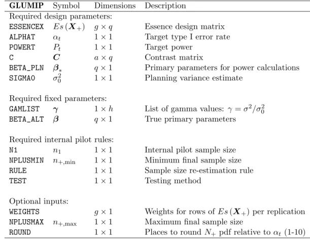
The following module names are used by the software, and hence should not be used by the user: _MAXTSB, _FINDADJB,_GLUMIP, _FCTS1, _FCTS2, _FCTT,_GETPOW,_QUAD2D01,_NDIST, _FINDADJ, _MAXTS, and _N2CALC. With 27 exceptions, all matrices used within the modules are locally defined, so there is no possibility of accidentally redefining a user-defined matrix. The exceptions are the required input matrices (SIGMA0, SIGHAT1, ALPHAT, POWERT, C, N1, BETA_PLN,ESSENCEX,BETA_ALT,GAMLIST,NPLUSMIN,RULE,TEST), the optional input matrices (NPLUSMAX, ROUND,WEIGHTS), the output matrices (_IPCALCS,_IPNAMES,_MAXTS,_MAXTSNM, _FINDADJ,_FINDADJNM,_N2CALCS,_N2CALCNM) and the matrices of parameters necessary for invoking the algorithms (GLOBAL1,GLOBAL2,_ZERO_).

GLUMIP Symbol Dimensions Description Required design parameters:

ESSENCEX Es(X+) g×q Essence design matrix

ALPHAT αt 1×1 Target type I error rate

POWERT Pt 1×1 Target power

C C a×q Contrast matrix

BETA_PLN β_∗ q×1 Primary parameters for power calculations

SIGMA0 σ2₀ 1×1 Planning variance estimate

Required fixed parameters:

GAMLIST γ 1×h List of gamma values: γ =σ2/σ₀2

BETA_ALT β q×1 True primary parameters

Required internal pilot rules:

N1 n1 1×1 Internal pilot sample size

NPLUSMIN n+,min 1×1 Minimum final sample size

RULE 1×1 Sample size re-estimation rule

TEST 1×1 Testing method

Optional inputs:

WEIGHTS g×1 Weights for rows of Es(X+) per replication

NPLUSMAX n+,max 1×1 Maximum final sample size

ROUND 1×1 Places to round N+ pdf relative toαt (1-10)

Table 1: Program inputs (with notation from Coffey and Muller 2001).

Table1summarizes the notation. SeeCoffey and Muller(1999,2001) orCoffeyet al.(2007) for additional details. The table also provides the corresponding variable names in theGLUMIP

program. The user must specify the design parameters for the initial power calculation. These include scalars for the initial variance estimate (SIGMA0), target type I error rate (ALPHAT), and target power (POWERT), a column vector of primary planning parameters used for sample size calculations (BETA_PLN), anessence matrix (ESSENCEX), and contrast matrix (C) for the initial power calculation. Note that these parameters are simply those that would be required for a power calculation in a fixed sample setting. The user must also specify a column vector containing the true matrix of primary parameters (BETA_ALT) and a list of gamma values (GAMLIST, where gamma is the ratio of the true variance to the variance value used for planning) to be used in the power calculations. The program tolerates definingGAMLIST as either a row or column vector. Finally, the user must specify the internal pilot specifications to be utilized for the chosen study. These consist of scalars for the choice of internal pilot sample size (N1), the minimum allowable size of the final sample (NPLUSMIN), the sample size re-estimation rule to apply (RULE), and the method for hypothesis testing (TEST).

By default the program performs computations assuming a balanced design with no finite upper bound on the final sample size. The user may choose to modify this by supplying one or more optional matrices. The user can specify a scalar (NPLUSMAX) to define a maximum allowable final sample size. In addition, the user can specify ROUND, a value between 1 and

10. This value determines when probabilities are sufficiently small to stop calculating the pdf of the final sample size for the largest value inGAMLIST. To allow for purposefully unbalanced designs, the user can specify a vector of weights (WEIGHTS) for each row of ESSENCEX per replication. For example, in a two group comparison where it is desired to maintain a 2:1 ratio in group 1 vs. group 2, one would choose a 2×2 identity matrix for ESSENCEX along with the following weight vector: WEIGHTS={2 1}‘;. Note that the replication factor m is calculated by the program as the sum of the elements of the WEIGHTS vector. For this unbalanced design, this implies thatm= 3 while in a corresponding balanced design,m= 2 is the number of independent groups. This factor does not ever have to be specified and WEIGHTSdoes not have to be specified for balanced designs.

The current version of the software has a limited error checking capacity. GLUMIP 2.0 will check to make sure that all required inputs are valid. If an invalid input is encountered (e.g., a negative variance), the program will stop and warn the user.

2.4. How the program works

TheGLUMIPpackage can be called from the user’sSAS/IMLprogram by any of four different commands: RUN GLUMIP;,RUN MAXTS;, orRUN FINDADJ;orRUN N2CALC;. TheRUN GLUMIP; command accesses the software’s main module, which calls on other modules to perform various tasks and functions.

If theRUN GLUMIP; command is given, the program first determines whatα value to use for critical value calculations associated with the final test statistic. For all tests (TEST=0, 1, 2, or 4) other than the bounding test (TEST=3), this is simply the target level input to the program (ALPHAT). If the bounding test is selected, the program uses the_FINDADJmodule to determine the adjusted level of alpha to use for determining the critical value such that the maximum type I error rate as a function ofγ will equalALPHAT. The_FINDADJmodule begins by calling the_MAXTS module to determine maximum type I error rate at the specified value ofALPHAT. Linear interpolation is then used as an initial guess for the requiredαadjustment, along with +/- 10% on either side. The algorithm then uses a doubly iterative search to find the desired adjustment. The inner iteration calls the _MAXTS module to determine the maximum type I error rate at a specified value ofα (which changes during each loop). The outer iteration searches for the adjusted α_* value such that the maximum type I error rate acrossγequalsαt. Success of the outer iteration depends directly on the accuracy in achieving

type I error rate bounded at or belowαt. The outer iteration continues until either 1)α* ≤αt

is found with maximum type I error rate sufficiently close in relative difference to αt, or 2)

the lower and upper limits ofα* are sufficiently close to each other relative toαt. In the first

case, theα* value is returned. In the latter case, the lower limit is returned.

For all tests (TEST=0, 1, 2, 3, or 4), following selection of the α value for critical value calculations, the program determines the distribution of the final sample size for the maximum value in the GAMLIST vector. This process uses the _NDIST module and depends on the specified re-estimation rule (RULE). The distribution of the final sample size is obtained by noting the monotone relationship between the final sample size,n+, and the variance estimate

obtained from the internal pilot sample, _bσ₁2. For each possible value of n+, the program

determines the cut point of bσ 2

1 that, if used in a sample size calculation, would lead to a

sample size less than or equal ton+ (Coffey and Muller 1999, 2001). This process continues

sample size greater or equal to the current value ofn+ falls below some threshold defined by

αt·10−ROUND (by default ROUND is 3). The program then begins looping through each of the

other specified values in GAMLIST. For each γ value, the process described above is applied until the algorithm first encounters the maximum final sample size specified by the user, the sample size at which the algorithm stopped for the maximum value inGAMLIST, or the current value ofn+ falls below some threshold defined by αt·10−(ROUND+2).

The distribution obtained from_NDISTis used to calculate the expected final sample size and is used in the_GETPOWmodule to compute the exact power under an internal pilot design for the specified testing method. ForTEST=0,1,2, or4, the critical value is obtained by choosing the 1−αtpercentile of an appropriateF distribution. IfTEST=3(the bounding test), the program

uses the adjusted alpha level returned by the _FINDADJfunction for determining the critical value. The power calculation consists of two stages. In the first stage, we condition onn+and

perform appropriate calculations. ForTEST=0or3, theSAS/IMLQUADfunction is used along with either the _FCTT module (if n+ =n1) or the _FCTS1 and _FCTS2 modules to integrate

the CDF of the test statistic across the cut points for each possiblen+ value determined from

_NDIST. For TEST=1, the QUAD function is used along with the _FCTT module to integrate the CDF. ForTEST=2, the test statistic conditionally follows an F distribution and only the SDF function is required for the conditional calculation. ForTEST=4, the_QUAD2D01 module is used to invoke theDavis and Rabinowitz(1984) method of numerical integration to perform 2D numerical integration of the quantile transformed integrand of the test statistic. Finally, the_GETPOWmodule returns the unconditional power determined by applying the law of total probability and summing over all possible values for the final sample size.

The _GLUMIP module repeats the above for each value specified in GAMLIST. After looping through all values, the module returns a matrix, _IPCALCS, that has one row for each value inGAMLIST and eleven columns corresponding to the values forALPHAT, the alpha value used to compute the critical value (equal to ALPHAT unless the bounding test is used), POWERT, GAMMA, N1,NPLUSMIN,NPLUSMAX(the SAS missing value .I is returned if no finite maximum sample size is specified),RULE,TEST, expected sample size, and power (or type I error rate if under null hypothesis). The program also returns a matrix,_IPNAMES, which contains column labels useful when printing the _IPCALCS matrix. These matrices are available to the user for further manipulation until the next RUN GLUMIP; command is issued. If the user wants to keep these values after an additional invocation of GLUMIP, they should be stored in matrices with distinct names before reissuing theRUN GLUMIP; command, or the results will be lost.

In some extreme cases, all of the probability may lie in one value for the final sample. For example, consider a case where no reduction in the planned sample size is allowed but we have dramatically overstated the true variance during planning. It may follow that the original planned sample size will be observed with a probability of 1. In such situations, we effectively have a fixed sample size and calculations can be simplified and based on an appropriate F distribution.

This software was written and has run successfully underSAS 9.1.3 using the Microsoft PC-Windows operating system.

2.5. Additional useful functions

deter-mining the maximum type I error rate as a function ofγ when using the unadjusted method. This command requires the same design parameters and internal pilot rules (except forRULE and TEST) as the RUN GLUMIP; command. The RUN MAXTS; command accesses the main module, which calls on the_MAXTSBand_MAXTS modules to implement an optimal Fibonacci algorithm to determine the maximum type I error rate for the given set of inputs. This com-mand produces a list: _MAXTS, which contains the value of γ at which the maximum type I error rate occurs, the maximum type I error rate, and the ratio of the maximum type I error rate to the target type I error rate. The module also produces _MAXTSNM, a list of column labels useful when printing _MAXTS. See Section 3.1 or 3.2 for use of the MAXTS module in examples.

If the user wants to implement a bounding test to protect against type I error rate inflation, theGLUMIP program provides the RUN FINDADJ; command as a stand alone option. The command finds an adjusted alpha level to ensure that the maximum type I error rate (over possible values ofγ) is no larger thanALPHAT. The same design parameters and internal pilot rules as theRUN GLUMIP;command are required except forRULEandTEST. TheRUN FINDADJ; command accesses the main module, which calls on the_FINDADJB and _FINDADJ modules. This command returns a scalar value,_FINDADJ, which contains the adjusted alpha value and _FINDADJNM, a column label useful when printing the returned value. See Section 3.2for use of theFINDADJ module in an example.

The GLUMIP program provides the RUN N2CALC; command as a stand alone option for determining the second stage sample size needed during study implementation. This command requires the same design parameters and internal pilot rules (except forTESTand SIGMA0) as theRUN GLUMIP; command. Additionally, the first sample error variance estimate (SIGHAT1) is a necessary input. TheRUN N2CALC; command accesses the main module, which calls on the_N2CALCmodule to implement the necessary sample size calculations.

The code determines the second stage sample size in the following manner. For each can-didate value for the second stage sample size (increasing by replication factorm), a critical value is determined using the given sample size re-estimation rule (RULE). Next, the minimum noncentrality factor needed for significance of the final test is calculated. From this noncen-trality, assuming the effect size of interest, a cut-off for a sufficiently low variance value is determined and the program stops if the first sample variance estimate is less than or equal to this value. Otherwise the program increases the sample size until either the condition is met, or the maximum sample size (NPLUSMAX) is attained.

This command produces a list: _N2CALCS, which containsSIGHAT1,N1,RULE,N2CALC(second stage sample size),NPLUSCALC(total sample size), and the projected power of the study using the given total sample size. The module also produces _N2CALCNM, a list of column labels useful when printing_N2CALCS. See Section3.5for use of the N2CALC module in an example.

2.6. Calling the program from a user written module

The software can also be run by using a CALL statement. This allows using the GLUMIP

software within other modules. Note that theGLUMIPinput matrices must all be specified as global variables in the modules referring to them. The following incomplete code (Program1) illustrates how to define a user module that calls theGLUMIP software.

START user_defined_module (parm1, parm2, ... parmn)

GLOBAL (ESSENCEX, ALPHAT, POWERT, C, BETA_PLN, SIGMA0, N1 NPLUSMIN, GAMLIST, BETA_ALT, RULE, TEST, WEIGHTS, NPLUSMAX, ROUND);

*some of your code here;

RUN _GLUMIP(_IPCALCS,_IPNAMES); *some more of your code here; FINISH user_defined_module;

Program 1: CallingGLUMIP from user-written module.

3. Example programs

We illustrate the usefulness of our code by reproducing results reported in four journal articles and one textbook. With the exception of our own works, the original published results were based on simulations. However, power calculation via simulation should only be a last resort since simulations have many practical disadvantages when compared to exact or approximate methods. Specifically, simulations typically require large amounts of computer time and each slight design change requires waiting for a new set of simulations to run. These limitations are worsened by the additional dimensions of study design created by the introduction of an internal pilot design. (Due to the fact that we are re-estimating the sample size at the internal pilot phase, a power calculation is embedded in the internal pilot phase. Hence simulating the power of an internal pilot design conditional on a particular first stage sample size requires, in essence, a simulation embedded in a simulation.) The output given are results using exact theory embedded in theGLUMIPprogram that are fast, stable, and accurate, thus removing the need to conduct simulations.

3.1. Example from Wittes and Brittain (1990) paper

A two group comparison previously described in Wittes and Brittain (1990) illustrates the use of the software. For this example with αt = 0.05, Pt = 0.90, θ∗ = 1 and σ20 = 2, a

fixed sample size power calculation suggests 43 subjects per group (n0= 86). We consider

an internal pilot design with 22 subjects per group in the internal pilot sample (n1= 44),

no finite maximum sample size, and no reduction of the final sample size if the variance was originally overstated (n+,min= 86). Program 2 invokes the RUN GLUMIP; command to

reproduce the power calculations reported in Table I of theWittes and Brittain(1990) paper and Table II of the Coffey and Muller (1999) paper. For all examples displayed here, the

GLUMIP code is attached using a SASmacro variable (&PROGPATH) to point to the directory where the GLUMIP 2.0 program is saved. For instance, all of the examples displayed here assume that the GLUMIP source code is saved in the H:\GLUMIPZIP\IML directory on the user’s hard drive. Please note that this line of code will need to be changed to point to the directory where the GLUMIP 2.0 program is saved on the user’s computer. The user must then provide values for all required inputs and any optional inputs desired. Using the /NOSOURCE2 option prevents the hundreds of lines of GLUMIP code from appearing in the SASlog. TheRUN GLUMIP;command begins execution of the GLUMIPprogram. Program2

* User must change next line to point to the directory where the GLUMIP program is saved;

%LET PROGPATH = C:\GLUMIP\IML; PROC IML WORKSIZE=1000 SYMSIZE=300;

RESET FUZZ FW=5;

%INCLUDE "&PROGPATH.\GLUMIP20.IML" / NOSOURCE2; ESSENCEX = I(2); ALPHAT = .05; POWERT = .90; C = {-1 1}; BETA_PLN = {0 1}`; SIGMA0 = 2; N1 = 44; GAMLIST = {.5 .75 1 1.5 2}; BETA_ALT = {0 1}`; TEST = 0; RULE = 0; NPLUSMIN = 86; RUN GLUMIP; PRINT _IPCALCS[COLNAME=_IPNAMES]; QUIT;

Program 2: Power calculations for Wittes and Brittain example.

generates the following output, indicating that the internal pilot design successfully maintains power at the target level of 0.90 regardless of the true value of the variance.

ALPHAT CRITVAL POWERT GAMMA N1 NPLUSMIN NPLUSMAX RULE TEST E(N) POWER

0.05 0.05 0.9 0.5 44 86 I 0 0 86 0.996

0.05 0.05 0.9 0.75 44 86 I 0 0 86.6 0.964

0.05 0.05 0.9 1 44 86 I 0 0 93.8 0.923

0.05 0.05 0.9 1.5 44 86 I 0 0 129.4 0.896

0.05 0.05 0.9 2 44 86 I 0 0 171.1 0.892

Program3invokes theRUN GLUMIP;command to reproduce the type I error rate calculations for this same example. Note that BETA_ALT, the vector of true parameters, takes the null vector value of02 for this calculation. Program 3generates the following output.

ALPHAT CRITVAL POWERT GAMMA N1 NPLUSMIN NPLUSMAX RULE TEST E(N) POWER

0.05 0.05 0.9 0.5 44 86 I 0 0 86 0.0500

0.05 0.05 0.9 0.75 44 86 I 0 0 86.6 0.0501

0.05 0.05 0.9 1 44 86 I 0 0 93.8 0.0510

0.05 0.05 0.9 1.5 44 86 I 0 0 129.4 0.0518

* User must change next line to point to the directory where the GLUMIP program is saved;

%LET PROGPATH = C:\GLUMIP\IML; PROC IML WORKSIZE=1000 SYMSIZE=300;

RESET FUZZ FW=6;

%INCLUDE "&PROGPATH.\GLUMIP20.IML" / NOSOURCE2; ESSENCEX = I(2); ALPHAT = .05; POWERT = .90; C = {-1 1}; BETA_PLN = {0 1}`; SIGMA0 = 2; N1 = 44; GAMLIST = {.5 .75 1 1.5 2}; BETA_ALT = {0 0}`; TEST = 0; RULE = 0; NPLUSMIN = 86; RUN GLUMIP; PRINT _IPCALCS[COLNAME=_IPNAMES]; QUIT;

Program 3: Type I error rates for Wittes and Brittain example.

While the results above suggest that type I error rate inflation is not a significant issue, we only observed the type I error rate for 5 specific values ofγ. If one were able to determine a priori that the maximum inflation of type I error rate was so small as not to cause any concern, researchers could gain the benefits of the internal pilot using the unadjusted method without having to worry about potential problems with type I error rate inflation. Program4 invokes theRUN MAXTS;command to determine the extent of potential type I error rate inflation for this example.

Program4generates the following output, indicating the maximum type I error rate of 0.0518 occurs atγ = 1.4425. Hence, for this example, the maximum amount of type I error rate in-flation is a little under 4% and no adjustment may be required. As a consequence, researchers could ignore the randomness of the final sample size and use most standard statistical software packages at the analysis phase.

_MAXTS

GAMMA(MAX) MAX TYPE I ERR. RATE RATIO: MAX/ALPHAT

1.4425 0.0518 1.0369

(n1= 44), no finite maximum sample size, and no reduction of the final sample size if the

* User must change next line to point to the directory where the GLUMIP program is saved;

%LET PROGPATH = C:\GLUMIP\IML; PROC IML WORKSIZE=1000 SYMSIZE=300;

RESET FUZZ FW=6;

%INCLUDE "&PROGPATH.\GLUMIP20.IML" / NOSOURCE2; ESSENCEX = I(2); ALPHAT = .05; POWERT = .90; C = {-1 1}; BETA_PLN = {0 1}`; SIGMA0 = 2; N1 = 44; NPLUSMIN = 86; RUN MAXTS; PRINT _MAXTS[COLNAME=_MAXTSNM]; QUIT;

Program 4: Maximum type I error rate for Wittes and Brittain example.

In Program 5, we slightly alter the example from Wittes and Brittain (1990) in order to exemplify the use of unbalanced groups for power and expected sample size calculations with theGLUMIP 2.0 software. We will assume a 2:1 unbalanced two group design, which might be considered if a new treatment were more expensive than the control treatment. With the same effect size and planning variance used, the fixed sample, unbalanced design requires 96 subjects (n0 = 96). The internal pilot sample will use 48 subjects (n1 = 48) with

the minimum final sample size not allowed to decrease (n+,min = 96). Note the addition of

the WEIGHTS = {2 1}‘; line to the program to specify the non-default unbalanced design preference. Program5 generates the following output for the unbalanced design.

ALPHAT CRITVAL POWERT GAMMA N1 NPLUSMIN NPLUSMAX RULE TEST E(N) POWER

0.05 0.05 0.9 0.5 48 96 I 0 0 96 0.995

0.05 0.05 0.9 0.75 48 96 I 0 0 96.7 0.963

0.05 0.05 0.9 1 48 96 I 0 0 104.8 0.922

0.05 0.05 0.9 1.5 48 96 I 0 0 145.6 0.896

0.05 0.05 0.9 2 48 96 I 0 0 192.6 0.893

3.2. Example from Coffey and Muller (2001) paper

We revisit the CLAHE example (Pisano et al. 1998) described in Section 1.2 and used in Coffey and Muller (2001) to demonstrate the performance of various methods of control-ling type I error rate while gaining the benefits of an internal pilot design. Specifically, we consider an internal pilot design with the following specifications: 1) a pre-planned sample

* User must change next line to point to the directory where the GLUMIP program is saved;

%LET PROGPATH = C:\GLUMIP\IML; PROC IML WORKSIZE=1000 SYMSIZE=300;

RESET FUZZ FW=5;

%INCLUDE "&PROGPATH.\GLUMIP20.IML" / NOSOURCE2; ESSENCEX = I(2); WEIGHTS = {2 1}`; ALPHAT = .05; POWERT = .90; C = {-1 1}; BETA_PLN = {0 1}`; SIGMA0 = 2; N1 = 48; GAMLIST = {.5 .75 1 1.5 2}; BETA_ALT = {0 1}`; TEST = 0; RULE = 0; NPLUSMIN = 96; RUN GLUMIP; PRINT _IPCALCS[COLNAME=_IPNAMES]; QUIT;

Program 5: Power calculations for unbalanced Wittes and Brittain example.

size of n0 = 20 radiologists, 2) the first n1 = 10 radiologists comprise the internal pilot

sample (N1=10), 3) the final sample size is allowed to decrease if the original variance value overestimates the true variance (NPLUSMIN=10), and 4) a finite upper bound of n+,max = 30

radiologists (NPLUSMAX=30). Program 6 invokes the RUN MAXTS;command to determine the maximum type I error rate using the unadjusted method for the CLAHE example in this setting. Program6generates the following output, indicating the maximum type I error rate of 0.0019 occurs atγ= 1.70:

_MAXTS

GAMMA(MAX) MAX TYPE I ERR. RATE RATIO: MAX/ALPHAT

1.7037 0.0019 1.695

Hence, for this example, ignoring the randomness of the final sample size introduced by using an internal pilot design could lead to as much as a 70% inflation of the target type I error rate. In such situations, one should attempt to maintain the benefits of an internal pilot design while controlling type I error rate using one of the methods described inCoffey and Muller (2001).

The bounding method provides one option for controlling the type I error rate for this example. Program 7 invokes the RUN _FINDADJ; command to determine the adjusted alpha value to

* User must change next line to point to the directory where the GLUMIP program is saved;

%LET PROGPATH = C:\GLUMIP\IML; PROC IML WORKSIZE=1000 SYMSIZE=300;

RESET FUZZ FW=6;

%INCLUDE "&PROGPATH.\GLUMIP20.IML" / NOSOURCE2; ESSENCEX = I(1); ALPHAT = .0011; POWERT = .90; C = {1}; BETA_PLN = {0.10}; SIGMA0 = .0065; N1 = {10}; NPLUSMIN = N1; NPLUSMAX = 30; RUN MAXTS; PRINT _MAXTS[COLNAME=_MAXTSNM]; QUIT;

Program 6: Maximum type I error rate for Coffey and Muller example. * User must change next line to point to the directory

where the GLUMIP program is saved; %LET PROGPATH = C:\GLUMIP\IML;

PROC IML WORKSIZE=1000 SYMSIZE=300; RESET FUZZ FW=6;

%INCLUDE "&PROGPATH.\GLUMIP20.IML" / NOSOURCE2; ESSENCEX = I(1); ALPHAT = .0011; POWERT = .90; C = {1}; BETA_PLN = {0.10}; SIGMA0 = .0065; N1 = {10}; NPLUSMIN = N1; NPLUSMAX = 30; RUN FINDADJ; PRINT _FINDADJ[COLNAME=_FINDADJNM]; QUIT;

* User must change next line to point to the directory where the GLUMIP program is saved;

%LET PROGPATH = C:\GLUMIP\IML; PROC IML WORKSIZE=1000 SYMSIZE=300;

RESET FUZZ FW=6;

%INCLUDE "&PROGPATH.\GLUMIP20.IML" / NOSOURCE2; ESSENCEX = I(1); ALPHAT = .0011; POWERT = .90; C = {1}; BETA_PLN = {.10}; SIGMA0 = .0065; N1 = {10}; GAMLIST ={.5 1 2}; BETA_ALT = {.10}; NPLUSMAX = 30; DO TEST=0 TO 3;

IF TEST=2 THEN NPLUSMIN=12; ELSE NPLUSMIN=10;

IF TEST=3 THEN RULE=0; ELSE RULE=TEST; RUN GLUMIP;

PRINT _IPCALCS[COLNAME=_IPNAMES]; END;

QUIT;

Program 8: Power calculations for Coffey and Muller example.

use for determining the critical value. Program 7 generates the following output, indicating that the critical value for the bounding test should be computed usingα∗= 0.0006.

_FINDADJ Adjusted Alpha

0.0006

In general, if the analysis calls for a final sample size n+, the critical value for a one group

ttest for a givenαcan be writtentcrit=Ft−1(1−α/2, n+−1). For this example, ifn+= 20 is

determined, this translates to using an adjusted critical value oftcrit=Ft−1(1−0.0006/2,19) =

4.11 while the unadjusted test withα= 0.0011 would usetcrit=Ft−1(1−0.0011/2,19) = 3.84.

However, the bounding test is not the only option for controlling the type I error rate. Rows 4–6 of Table 2 in Coffey and Muller (2001) provided some results for expected sample size and power when applying Methods 0/0, 1/1, 2/2, and 0/3 to the CLAHE example with these internal pilot rules. Program8usesGLUMIP 2.0 to reproduce the calculations in addition to

including calculations for Method 2/2. In the current version of the software,RULEand TEST must be scalar values. Hence, we had to write our own DO-END loop to compute the power and expected sample size for multiple combinations of the two. In addition, note that when using Method 2/2, we must set NPLUSMIN=12 to ensure that we have enough observations in the second sample to compute an estimate of the variance. Program 8produces the following results, which clearly agree with the results shown in rows 4–6 of Table 2 inCoffey and Muller (2001):

ALPHAT CRITVAL POWERT GAMMA N1 NPLUSMIN NPLUSMAX RULE TEST E(N) POWER

0.0011 0.0011 0.9 0.5 10 10 30 0 0 12.7 0.9709

0.0011 0.0011 0.9 1 10 10 30 0 0 18.9 0.9134

0.0011 0.0011 0.9 2 10 10 30 0 0 26.4 0.7916

ALPHAT CRITVAL POWERT GAMMA N1 NPLUSMIN NPLUSMAX RULE TEST E(N) POWER

0.0011 0.0011 0.9 0.5 10 10 30 1 1 14.9 0.9761

0.0011 0.0011 0.9 1 10 10 30 1 1 23.8 0.8953

0.0011 0.0011 0.9 2 10 10 30 1 1 28.9 0.5534

ALPHAT CRITVAL POWERT GAMMA N1 NPLUSMIN NPLUSMAX RULE TEST E(N) POWER

0.0011 0.0011 0.9 0.5 10 10 30 2 2 17.7 0.8571

0.0011 0.0011 0.9 1 10 10 30 2 2 22.6 0.8239

0.0011 0.0011 0.9 2 10 10 30 2 2 27.8 0.7266

ALPHAT CRITVAL POWERT GAMMA N1 NPLUSMIN NPLUSMAX RULE TEST E(N) POWER

0.0011 0.0006 0.9 0.5 10 10 30 0 3 12.7 0.9438

0.0011 0.0006 0.9 1 10 10 30 0 3 18.9 0.8728

0.0011 0.0006 0.9 2 10 10 30 0 3 26.4 0.7298

3.3. Example from Proschan and Wittes (2000) paper

A two group comparison previously described in Proschan and Wittes(2000) withαt= 0.05,

Pt = 0.90, σ2 = 1, and θ∗ = 1 illustrates the performance of the weighted test. The

au-thors reported simulation results to evaluate the type I error rate and power of Stein’s test, the weighted test, and the unadjusted test for three different scenarios, corresponding to whether the prior estimate of the standard deviation was 25% low, on target, or 25% high

σ₀2 ∈0.5625,1.0,1.5625

. For these three scenarios, a fixed sample size power calculation sug-gests 12, 22, and 34 subjects per group, respectively (n0∈24,44,68). They considered an

in-ternal pilot design with one-half of the originally planned subjects included in the inin-ternal pilot sample (n1∈12,22,34), no finite maximum sample size, and no reduction of the final sample

size if the variance was originally overstated. Program 9invokes theRUN GLUMIP; command to reproduce the type I error rate calculations reported for Table 1 in theProschan and Wittes (2000) paper. Note that when TEST=4 is used, GLUMIP issues the following caution (not included in output): WARNING: TEST=4 is only appropriate when NPLUSMIN = N_not, the originally planned sample size. Otherwise interpret results with caution. Program 9 generates the following output.

* User must change next line to point to the directory where the GLUMIP program is saved;

%LET PROGPATH = C:\GLUMIP\IML; PROC IML WORKSIZE=1000 SYMSIZE=300;

RESET FUZZ FW=5;

%INCLUDE "&PROGPATH.\GLUMIP20.IML" / NOSOURCE2; TESTLIST = {1 4 0}; ESSENCEX = I(2); ALPHAT = .05; POWERT = .90; C = {-1 1}; BETA_PLN = {0 1}`; SIGLIST = {0.5625 1 1.5625}; N1LIST = {12 22 34}; GAMLISTB = {1.78 1 0.64}; NPMINLIST= {24 44 68}; RULE = 0; BETA_ALT = {0 0}`; DO I=1 TO NCOL(SIGLIST); SIGMA0 = SIGLIST[,I]; N1 = N1LIST[,I]; GAMLIST = GAMLISTB[,I]; NPLUSMIN = NPMINLIST[,I]; DO J=1 TO NCOL(TESTLIST); TEST = TESTLIST[,J]; RUN GLUMIP; OUT=OUT//_IPCALCS; END; END; PRINT OUT[COLNAME=_IPNAMES]; QUIT;

Program 9: Type I error rates for Proschan and Wittes example. OUT

ALPHAT CRITVAL POWERT GAMMA N1 NPLUSMIN NPLUSMAX RULE TEST E(N) POWER

0.05 0.05 0.9 1.78 12 24 I 0 1 45.6 0.05 0.05 0.05 0.9 1.78 12 24 I 0 4 45.6 0.047 0.05 0.05 0.9 1.78 12 24 I 0 0 45.6 0.055 0.05 0.05 0.9 1 22 44 I 0 1 49.7 0.05 0.05 0.05 0.9 1 22 44 I 0 4 49.7 0.05 0.05 0.05 0.9 1 22 44 I 0 0 49.7 0.052 0.05 0.05 0.9 0.64 34 68 I 0 1 68.1 0.05 0.05 0.05 0.9 0.64 34 68 I 0 4 68.1 0.05 0.05 0.05 0.9 0.64 34 68 I 0 0 68.1 0.05

To reproduce the power calculations for Table 1 in the Proschan and Wittes (2000) paper, the only change that is required to the above code is to replace the statement BETA_ALT = {0 0}‘; with the statement BETA_ALT = {0 1}‘;. The code (Program 10) generates the following output.

OUT

ALPHAT CRITVAL POWERT GAMMA N1 NPLUSMIN NPLUSMAX RULE TEST E(N) POWER

0.05 0.05 0.9 1.78 12 24 I 0 1 45.6 0.869 0.05 0.05 0.9 1.78 12 24 I 0 4 45.6 0.873 0.05 0.05 0.9 1.78 12 24 I 0 0 45.6 0.879 0.05 0.05 0.9 1 22 44 I 0 1 49.7 0.924 0.05 0.05 0.9 1 22 44 I 0 4 49.7 0.929 0.05 0.05 0.9 1 22 44 I 0 0 49.7 0.931 0.05 0.05 0.9 0.64 34 68 I 0 1 68.1 0.98 0.05 0.05 0.9 0.64 34 68 I 0 4 68.1 0.983 0.05 0.05 0.9 0.64 34 68 I 0 0 68.1 0.983

3.4. Example from Jennison and Turnbull (2000) textbook

In Table 14.4 of their textbook,Jennison and Turnbull (2000) reported simulation results to examine the mean total sample size, type I error rate, and power of the unadjusted test for comparing two means. For their example, they setαt = 0.05, Pt = 0.90, and θ∗ = 1. They

considered five different scenarios for the variance, but in each case they assume that the prior estimate of the variance is equal to the true, unknown value. For these five scenarios, a fixed sample size power calculation suggests 8, 12, 23, 44, and 86 subjects per group, respectively. They considered an internal pilot design with varying fractions of the originally planned subjects included in the internal pilot sample, no finite maximum sample size, and allowed the final sample size to be reduced if the variance was originally overstated. Program 11 invokes the RUN GLUMIP; command to reproduce the type I error rate calculations reported for Table 14.4 in the Jennison and Turnbull(2000) text. Program 11 generates the following output.

OUT

ALPHAT CRITVAL POWERT GAMMA N1 NPLUSMIN NPLUSMAX RULE TEST E(N) POWER

0.05 0.05 0.9 1 4 4 I 0 0 16 0.09 0.05 0.05 0.9 1 6 6 I 0 0 16 0.076 0.05 0.05 0.9 1 10 10 I 0 0 16.1 0.062 0.05 0.05 0.9 1 20 20 I 0 0 20.4 0.05 0.05 0.05 0.9 1 4 4 I 0 0 24.3 0.085 0.05 0.05 0.9 1 6 6 I 0 0 24.2 0.074 0.05 0.05 0.9 1 10 10 I 0 0 24.2 0.065 0.05 0.05 0.9 1 20 20 I 0 0 25.1 0.055 0.05 0.05 0.9 1 6 6 I 0 0 45.1 0.065 0.05 0.05 0.9 1 10 10 I 0 0 45.1 0.06 0.05 0.05 0.9 1 20 20 I 0 0 45.1 0.057 0.05 0.05 0.9 1 40 40 I 0 0 46.7 0.053

* User must change next line to point to the directory where the GLUMIP program is saved;

%LET PROGPATH = C:\GLUMIP\IML; PROC IML WORKSIZE=1000 SYMSIZE=300;

RESET FUZZ FW=5;

%INCLUDE "&PROGPATH.\GLUMIP20.IML" / NOSOURCE2; ESSENCEX = I(2); ALPHAT = .05; POWERT = .90; C = {-1 1}; BETA_PLN = {0 1}`; SIGLIST = {0.3 0.5 1.0 2.0 4.0}; RULE = 0; TEST = 0; N1LISTB = { 4 6 10 20, 4 6 10 20, 6 10 20 40, 6 10 20 40, 10 20 40 80}; GAMLIST = {1}; BETA_ALT = {0 0}`; DO I=1 TO NCOL(SIGLIST); SIGMA0 = SIGLIST[,I]; N1LIST = N1LISTB[I,]; DO J=1 TO NCOL(N1LIST); N1 = N1LIST[,J]; NPLUSMIN = N1; RUN GLUMIP; OUT=OUT//_IPCALCS; END; END; PRINT OUT[COLNAME=_IPNAMES]; QUIT;

Program 11: Type I error rates for Jennison and Turnbull example.

0.05 0.05 0.9 1 6 6 I 0 0 87.1 0.058 0.05 0.05 0.9 1 10 10 I 0 0 87 0.055 0.05 0.05 0.9 1 20 20 I 0 0 87 0.054 0.05 0.05 0.9 1 40 40 I 0 0 87 0.053 0.05 0.05 0.9 1 10 10 I 0 0 171.1 0.052 0.05 0.05 0.9 1 20 20 I 0 0 171.1 0.052 0.05 0.05 0.9 1 40 40 I 0 0 171.1 0.052 0.05 0.05 0.9 1 80 80 I 0 0 171.1 0.051

To reproduce the power calculations for Table 14.4 inJennison and Turnbull(2000), the only change that is required to the above code is to replace the statement BETA_ALT = {0 0}‘; with the statement BETA_ALT = {0 1}‘;. The code (Program 12) generates the following output.

OUT

ALPHAT CRITVAL POWERT GAMMA N1 NPLUSMIN NPLUSMAX RULE TEST E(N) POWER

0.05 0.05 0.9 1 4 4 I 0 0 16 0.83 0.05 0.05 0.9 1 6 6 I 0 0 16 0.893 0.05 0.05 0.9 1 10 10 I 0 0 16.1 0.931 0.05 0.05 0.9 1 20 20 I 0 0 20.4 0.977 0.05 0.05 0.9 1 4 4 I 0 0 24.3 0.782 0.05 0.05 0.9 1 6 6 I 0 0 24.2 0.852 0.05 0.05 0.9 1 10 10 I 0 0 24.2 0.897 0.05 0.05 0.9 1 20 20 I 0 0 25.1 0.931 0.05 0.05 0.9 1 6 6 I 0 0 45.1 0.811 0.05 0.05 0.9 1 10 10 I 0 0 45.1 0.862 0.05 0.05 0.9 1 20 20 I 0 0 45.1 0.898 0.05 0.05 0.9 1 40 40 I 0 0 46.7 0.921 0.05 0.05 0.9 1 6 6 I 0 0 87.1 0.787 0.05 0.05 0.9 1 10 10 I 0 0 87 0.842 0.05 0.05 0.9 1 20 20 I 0 0 87 0.88 0.05 0.05 0.9 1 40 40 I 0 0 87 0.898 0.05 0.05 0.9 1 10 10 I 0 0 171.1 0.832 0.05 0.05 0.9 1 20 20 I 0 0 171.1 0.871 0.05 0.05 0.9 1 40 40 I 0 0 171.1 0.89 0.05 0.05 0.9 1 80 80 I 0 0 171.1 0.899

3.5. 3-Group ANOVA Example from Coffey and Muller (1999) paper To illustrate the flexibility and usefulness of the GLUMIP software package, we consider a three-group analysis of variance (ANOVA) design described as Example C in Coffey and Muller(1999). For the two degree of freedom test of differences among groups withαt= 0.05,

Pt = 0.90, σ2 = 1, and θ∗ =0.5 1.0 0

, a fixed sample calculation suggests 27 observations per group. To mirror the results found in Coffey and Muller (1999), we consider the three-group ANOVA example for an internal pilot with the following specifications: 1) a pre-planned sample size of n0= 81, 2) the firstn1 = 39 (13 per group) observations comprise the internal

pilot sample (N1=39), 3) both allowing and not allowing the final sample size to decrease if the original variance value overestimates the true variance (NPLUSMIN=39 and NPLUSMIN=81, respectively), 4) no finite upper bound of observations, 5) using Unadjusted Method for sample size re-estimation and testing (RULE=0 and TEST=0). Program 13 invokes the RUN GLUMIP; command to reproduce the type I error rate results found in Coffey and Muller (1999, Table V).

* User must change next line to point to the directory where the GLUMIP program is saved;

%LET PROGPATH = C:\GLUMIP\IML; PROC IML WORKSIZE=1000 SYMSIZE=300;

RESET FUZZ FW=6;

%INCLUDE "&PROGPATH.\GLUMIP20.IML" / NOSOURCE2; ESSENCEX = I(3); ALPHAT = .05; POWERT = .90; C = {1 -1 0, 0 1 -1}; BETA_PLN = {0 0.5 1}`; SIGMA0 = 1; N1 = {39}; GAMLIST ={0.5 0.75 1 1.5 2}; BETA_ALT = {0 0 0}`; TEST=0; RULE=0; NPLUSMINLIST={81 39}; DO I=1 TO NCOL(NPLUSMINLIST); NPLUSMIN=NPLUSMINLIST[I]; RUN GLUMIP; PRINT _IPCALCS[COLNAME=_IPNAMES]; END; QUIT;

Program 13: Type I error rates for Coffey and Muller (1999) example.

_IPCALCS

ALPHAT CRITVAL POWERT GAMMA N1 NPLUSMIN NPLUSMAX RULE TEST E(N) POWER

0.05 0.05 0.9 0.5 39 81 I 0 0 81 0.05

0.05 0.05 0.9 0.75 39 81 I 0 0 81.6 0.0501

0.05 0.05 0.9 1 39 81 I 0 0 87.9 0.0512

0.05 0.05 0.9 1.5 39 81 I 0 0 119 0.0525

0.05 0.05 0.9 2 39 81 I 0 0 156.4 0.0522

ALPHAT CRITVAL POWERT GAMMA N1 NPLUSMIN NPLUSMAX RULE TEST E(N) POWER

0.05 0.05 0.9 0.5 39 39 I 0 0 44.5 0.0528

0.05 0.05 0.9 0.75 39 39 I 0 0 61.7 0.0556

0.05 0.05 0.9 1 39 39 I 0 0 80.5 0.0547

0.05 0.05 0.9 1.5 39 39 I 0 0 118.4 0.0531

To reproduce the power calculations for Table V inCoffey and Muller(1999), the only change that is required to the above code is to replace the statementBETA_ALT = {0 0 0}‘; with the statementBETA_ALT = {0 0.5 1.0}‘;. The code (Program 14) generates the following output.

OUT

ALPHAT CRITVAL POWERT GAMMA N1 NPLUSMIN NPLUSMAX RULE TEST E(N) POWER

0.05 0.05 0.9 0.5 39 81 I 0 0 81 0.9974

0.05 0.05 0.9 0.75 39 81 I 0 0 81.6 0.9709

0.05 0.05 0.9 1 39 81 I 0 0 87.9 0.9305

0.05 0.05 0.9 1.5 39 81 I 0 0 119 0.8976

0.05 0.05 0.9 2 39 81 I 0 0 156.4 0.8914

ALPHAT CRITVAL POWERT GAMMA N1 NPLUSMIN NPLUSMAX RULE TEST E(N) POWER

0.05 0.05 0.9 0.5 39 39 I 0 0 44.5 0.9325

0.05 0.05 0.9 0.75 39 39 I 0 0 61.7 0.9118

0.05 0.05 0.9 1 39 39 I 0 0 80.5 0.9038

0.05 0.05 0.9 1.5 39 39 I 0 0 118.4 0.8955

0.05 0.05 0.9 2 39 39 I 0 0 156.4 0.8913

The following program (Program 15) illustrates the use of the new (N2CALC) module for the three-group ANOVA example. The program will consider sample size calculations for various first sample variance estimates (SIGHAT1) using either the unadjusted or the Stein-like sample size re-estimation rules (RULE=0 or 1, respectively).

Program15 generates the following output, giving needed second stage sample sizes. N2CALCOUT

SIGMAHAT1 N1 RULE N2CALC NPLUSCALC Projected Power

0.5 39 0 3 42 0.9068 1 39 0 42 81 0.9077 1.5 39 0 78 117 0.9002 0.5 39 1 3 42 0.9049 1 39 1 45 84 0.9049 1.5 39 1 87 126 0.9049

4. Discussion

The results in Coffey and Muller(2001) extend many internal pilot design concepts from the t test setting to the classic general linear univariate model setting. The introduction of the

GLUMIP program further extends the practicability of internal pilot designs in two ways: 1. Researchers can examine the maximum inflation of type I error rate possible if an

internal pilot is used with the unadjusted test. This can allow a very quick and early determination as to whether type I error rate inflation should be a concern in any particular study.

* User must change next line to point to the directory where the GLUMIP program is saved;

%LET PROGPATH = C:\GLUMIP\IML; PROC IML WORKSIZE=1000 SYMSIZE=300;

RESET FUZZ FW=6;

%INCLUDE "&PROGPATH.\GLUMIP20.IML" / NOSOURCE2; ESSENCEX = I(3); ALPHAT = .05; POWERT = .90; C = {1 -1 0, 0 1 -1}; BETA_PLN = {0 0.5 1}`; N1 = {39}; NPLUSMIN=39; RULELIST={0 1}; SIG1LIST={0.5 1 1.5}; FREE N2CALCOUT; DO J=1 TO NCOL(RULELIST); RULE=RULELIST[J]; DO I=1 TO NCOL(SIG1LIST); SIGHAT1=SIG1LIST[I]; RUN N2CALC; N2CALCOUT=N2CALCOUT//_N2CALCS; END; END; PRINT N2CALCOUT[COLNAME=_N2CALCNM]; QUIT;

Program 15: N2 calculations for Coffey and Muller (1999) example.

2. When there is reason to be concerned about type I error rate inflation, investigators have several options as to how to control type I error rate and maintain the benefits of an internal pilot design. GLUMIP can allow investigators to examine the impact on power and sample size for each choice and make a decision to maximize the benefits of the internal pilot design for their particular study.

Furthermore, the new and much simpler density and cumulative distribution function forms included in this updated version make the bounding method more practical and convenient even in very small samples where it has the most value. The speed also allows quickly plotting power and expected sample size over wide ranges of design parameters. The ability to produce such plots in a timely manner has many advantages. For example, there is an obvious trade-off between choosing a large enough value of n1 to ensure a reliable estimate ofσ2 and choosing

the smallest possible value ofn1such that modifications to sample size, and any corresponding

logistical changes to the on-going study, can be implemented as early as possible. Historically, completely arbitrary values, such as n1 =n0/2, have been chosen. Examining plots of power

which retains the desired benefits of an internal pilot.

TheGLUMIP program is intended to aid in study planning when incorporating an internal pilot design. While the inclusion of theN2CALC facilitates study implementation, the current software does not fully support study analysis. However, with GLUMIP and careful use of other standard software, analysis can be implemented as follows.

1. UseGLUMIPto explore possible design parameters with respect to sample size, power, and type I error rate properties in order to determine appropriate design.

2. Use software such as POWERLIB (Johnson et al. 2008) to determine necessary fixed study sample size

3. Sample subjects needed for first stage according to design

4. Use N2CALC to calculate necessary second stage sample size according to sample size update rule (RULE) chosen at design stage

5. Perform usual analysis at final stage using desired variance estimate and testing proce-dure (TEST) chosen at design stage

Step 5 is straightforward with the unadjusted (TEST=0) or bounding (TEST=3) tests since they use the usual test statistic and critical value calculations involve only traditional forms using either the preplanned α (TEST=0) or the adjusted α∗ predetermined

us-ing the RUN _FINDADJ; command (TEST=3 in GLUMIP; see examples in Section 3.2). Implementation for the other three testing methods included for planning purposes in

GLUMIP 2.0 (TEST=1, TEST=2 or TEST=4) is more difficult. Since they do not use the usual test statistic in final analysis, the correct variance and degree of freedom compo-nents must be carefully picked off from appropriate locations and combined to create the necessary statistic and critical values. These testing methods would have the most to gain from the availability of additional analysis software.

Although we provide valid arguments for utilizing theGLUMIP2.0 software for internal pilot designs, users must be cautioned that this is still a work in progress. The user should consult the appropriate articles in the reference list to understand the limitations of the program. There are several ways in which we hope to improve the software in the future:

ˆ The current version includes only a subset of proposed methods for controlling the type I error rate in internal pilot designs. The versatility of the package will continue to grow by incorporating alternative methods into the software. This would especially include methods employing blinded sample size re-estimation techniques that have great appeal when mitigation of potential bias is crucial.

ˆ The software (and internal pilot results in general) are limited somewhat in that they have only been studied in the univariate setting. We are currently exploring ways to extend the internal pilot results to the repeated measures setting. As these methods are developed and published, we envision that a more general version of the software will become available with the univariate algorithms occurring as special cases.

ˆ The GLUMIP program does not currently perform full data analysis for internal pilot designs. We plan to simplify this task by including additional software for data analysis under an internal pilot in later versions of GLUMIP.