2018
Evaluation of statistical and process-based models
as nitrogen recommendation tools in maize
production systems
Laila Alejandra Puntel Iowa State University
Follow this and additional works at:https://lib.dr.iastate.edu/etd Part of theAgriculture Commons
This Dissertation is brought to you for free and open access by the Iowa State University Capstones, Theses and Dissertations at Iowa State University Digital Repository. It has been accepted for inclusion in Graduate Theses and Dissertations by an authorized administrator of Iowa State University Digital Repository. For more information, please [email protected].
Recommended Citation
Puntel, Laila Alejandra, "Evaluation of statistical and process-based models as nitrogen recommendation tools in maize production systems" (2018).Graduate Theses and Dissertations. 16655.
by
Laila Alejandra Puntel
A dissertation submitted to the graduate faculty in partial fulfillment of the requirements for the degree of
DOCTOR OF PHILOSOPHY
Major: Crop Production and Physiology
Program of Study Committee: Sotirios V. Archontoulis, Major Professor
John E. Sawyer Michael J. Castellano
Emily A. Heaton Kenneth J. Moore
The student author, whose presentation of the scholarship herein was approved by the program of study committee, is solely responsible for the content of this dissertation. The Graduate College will ensure this dissertation is globally accessible and will not permit alterations after a
degree is conferred.
Iowa State University Ames, Iowa
2018
“Wisdom is not a product of schooling but of the lifelong attempt to acquire it” Albert Einstein
TABLE OF CONTENTS
Page
LIST OF FIGURES ... vi
LIST OF TABLES ... viii
ACKNOWLEDGMENTS ... ix
ABSTRACT ...x
CHAPTER 1. OVERVIEW ...1
References ...6
CHAPTER 2. MODELING LONG-TERM CORN YIELD RESPONSE TO NITROGEN RATE AND CROP ROTATION...11
Abstract ... 11
Introduction ... 12
Objectives ... 15
Materials and Methods ... 16
Site, Weather, and Experimental Datasets ... 16
The APSIM Modeling Platform ... 17
APSIM Configuration and Calibration... 17
Blind-Phase Model Parameters and Set-Up ... 18
Model Calibration and Testing ... 19
Data Analysis ... 20
Estimation of the Annual Economic Optimum Nitrogen Rate ... 20
Estimation of Site Mean Economic Optimum Nitrogen Rate ... 22
Statistical Evaluation of Model Performance ... 22
Factors Affecting Optimal Nitrogen Rate Inter-Annual Variability ... 23
Results ... 23
Observed Corn and Soybean Yield Response to N Fertilizer, and Crop Rotation ... 23
Model Accuracy before and after Calibration ... 24
Simulation of Corn Yields ... 24
Simulation of Soybean Yields ... 28
Simulation of Optimum N Rate and Methods Comparison ... 29
Site Mean Optimum N Rate ... 29
Annual Optimum N Rate ... 30
Factors Causing Yearly Variability in Optimal Nitrogen Rate ... 31
Discussion ... 33
Calibration Strategy and Steps ... 33
APSIM Performance in Simulating Yields before and after Calibration ... 35
Modeling Optimal Nitrogen Rate ... 37
Causes of Optimal Nitrogen Rate Variability ... 40
Conclusion ... 41
Appendix ... 55
References ... 65
CHAPTER 3. A SYSTEMS MODELING APPROACH TO FORECAST CORN ECONOMIC OPTIMUM NITROGEN RATE ...66
Abstract ... 66
Introduction ... 67
Objectives ... 71
Materials and Methods ... 71
Experimental Data and Site Description ... 71
The APSIM Modeling Platform, Set Up, and Calibration ... 72
Forecasting Yields and EONR ... 73
Data Analysis ... 74
Estimation of the Annual Economic Optimum Nitrogen Rate ... 74
Statistical Evaluation of Model Performance ... 75
Statistical Evaluation of Weather Scenarios ... 76
Results ... 76
Yield Predictions at Different Forecasting Times Using 35 Years of Historical Weather ... 76
EONR Prediction at Different Forecasting Times Using 35 Year of Historical Weather ... 81
Assessing the Impact of Different Weather Scenarios ... 84
Comparison between APSIM and the 16 Year Site-Mean EONR and YEONR ... 85
Discussion ... 88
Yield Forecasts ... 88
EONR Forecast... 89
Future Improvements Toward More Accurate N Rate Forecasts ... 91
Conclusions ... 94
References ... 94
Appendix ... 102
CHAPTER 4. DEVELOPMENT OF A NITROGEN RECOMMENDATION TOOL FOR CORN CONSIDERING STATIC AND DYNAMIC VARIABLES ...109
Abstract ... 109
Introduction ... 110
Materials and Methods ... 112
Experimental sites and design ... 112
Measurements and data processing ... 113
Static variables ... 114
Dynamic variables ... 115
Data analysis... 116
Model validation ... 118
Results ... 118
Spatial and temporal variability of the explanatory variables ... 118
Temporal and spatial variability of EONR and yields ... 122
Relative importance of factors and model development ... 124
Model validation... 128
Discussion ... 129
Predicting corn optimum N rate ... 129
Factors affecting the EONR ... 131
Conclusions ... 134
References ... 135
Appendix ... 139
CHAPTER 5. CONCLUSIONS ...143
LIST OF FIGURES
Page Figure 1.1 Thesis diagram ... 6 Figure 2.1 Corn yield response to N fertilizer for the continuous corn (CC) cropping
system. ... 25 Figure 2.2 Corn yield response to N fertilizer for the soybean-corn (SC) cropping system. .... 26 Figure 2.3 Sixteen year mean crop yield response to N fertilizer rate (A, D, and G panels),
and observed versus simulated crop yields across years and N rate (B, C, E, F, H, and I). Points are observations or simulations, continuous lines are
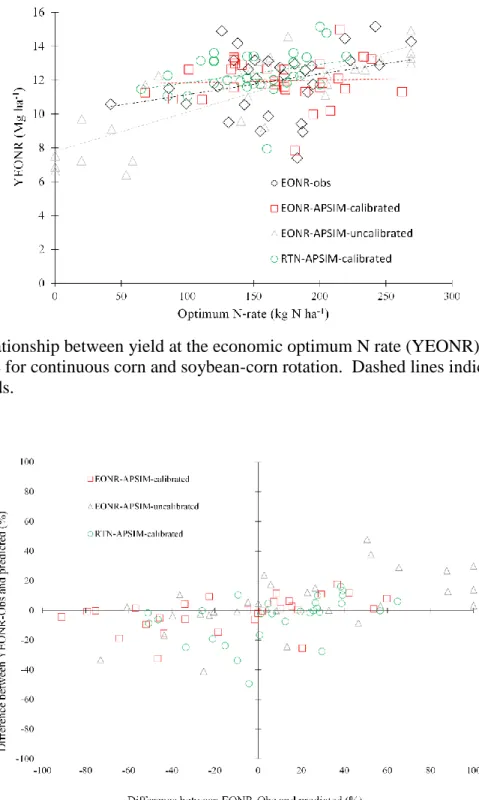
regression fits from Eqs. 1–3, and broken lines show 1:1 relationship. ... 27 Figure 2.4 Economic optimum N rate (EONR) and corn yield at the EONR (YEONR) for
every year in CC and SC. The EONR and YEONR estimates from
observations using Eqs. 1-3 are shown as bars. ... 28 Figure 2.5 Cumulative spring precipitation from April 1st to June 30th (every year) versus
economic optimum N rate ... 32 Figure 3.1 Overview of the main factors influencing the economic optimum nitrogen
fertilizer (EONR) rate and their interactions. Soil organic matter (SOM). ... 68 Figure 3.2 Simulated vs. observed corn yield (Top panel), economic optimum N rate
(Bottom panel, EONR), and yield at EONR (Central panel, YEONR) at
different corn stages using 35-yr weather data. ... 78 Figure 3.3 Predicted and observed yield at the economic optimum N rate (YEONR) for
continuous corn. ... 79 Figure 3.4 Predicted and observed yield at the economic optimum N rate (YEONR) for
soybean-corn. ... 80 Figure 3.5 Predicted and observed economic optimum N rate (EONR) for corn-corn. ... 82 Figure 3.6 Predicted and observed economic optimum N rate (EONR) for soybean-corn. ... 83 Figure 3.7 Differences in relative root mean square error (RRMSE) between weather
scenarios (I-V) and standard approach (use of 35-years of weather data) for predicted corn yield (A) and economic optimum N rate (B) at four forecasted times: planting ... 85
Figure 3.8 Distribution of differences between simulated economic optimum N rate (EONR) at planting time, V6 (6th leaf), V12 (12th leaf), R1 (silking), and R6 (maturity) growth stages, and the site-mean EONR minus the yearly observed EONR for continuous corn (CC) and soybean corn (SC) rotation. ... 87 Figure 4.1 Daily precipitation in Central West Buenos Aires, Argentina (top panel) and
cumulative precipitation for selected periods (bottom panel). ... 119 Figure 4.2 Nitrate-N content from 0 to 60 cm depth, water as percent of field capacity
from 20 to 60 cm soil depth (FC), soil water from 0 to 60 cm depth (SW_sum), soil organic matter at 20 cm depth (OM_20), water table depth at planting, and sand content at 20 cm depth (Sand_20). ... 120 Figure 4.3 Observed economic optimum nitrogen rate (EONR), yield at EONR
(YEONR), and yield at nitrogen zero (Yield_N0, right panels) and frequency distribution (right panels). Horizontal dashed lines represent the overall mean value. The coefficient of variation (CV%) for each season is provided. ... 123 Figure 4.4 Economic optimum N rate (EONR) as a function of yield at EONR (YEONR),
yield at N zero (Yield_N0), and the difference between YEONR and Yield_N0.. 124 Figure 4.5 Diagram of regression models for the economic optimum nitrogen rate (a),
yield at the EONR (b), and Yield at N0 (c) using static variables, dynamic variables, and a combination of both. Predicted versus observed values for the
full models are shown. ... 126 Figure 4.6 Relative importance of the static and dynamic variables included in the
reduced models. Left panel shows variables included in the EONR model,
middle panel in the YEONR model, and right panel the Yield_N0 model ... 127 Figure 4.7 Predicted versus observed economic optimum N rate (EONR), yield at EONR
(YEONR), and yield at non fertilizer (Yield_N0) for the validation data set using full model (circles) and reduced model (triangles). Diagonal dashed line shows 1:1 relationship. MAE is the mean absolute error. ... 129
LIST OF TABLES
Page Table 2.1 Mean economic optimum N rate (EONR, kg N ha-1) across 16-years for:
observed, Obs; un-calibrated Agricultural Production Systems sIMulator (APSIM) model, Unc; calibrated model, Cal; and the return to N approach
from the calibrated model, RTN. ... 29 Table 2.2 Statistical evaluation of the uncalibrated and calibrated APSIM model
performance in simulating corn and soybean yields by N rate across 16-years. ... 35 Table 3.1 Site-mean and the associated standard deviation economic optimum N rate
(EONR, units: kg N ha-1) for each crop rotation, forecast time, and the
measured site-mean across years. ... 81 Table 3.2 Comparison of economic optimum nitrogen rate (EONR) estimated by APSIM
to the site mean EONR and observed EONR for continuous corn and soybean-corn over three categorical EONR ranges. ... 87 Table 4.1 Description of static and dynamic explanatory variables. ... 121 Table 4.2 Full and reduced regression models for the economic optimum nitrogen rate
(EONR; units: kg N ha-1), yield at EONR (YEONR; Mg ha-1), and yield at
nitrogen zero (Yield_N0; Mg ha-1) ... 125 Table 4.3 Mean absolute error for economic optimum nitrogen rate (EONR; units: kg N
ha-1), yield at EONR (YEONR; Mg ha-1), and yield at zero nitrogen
(Yield_N0; Mg ha-1) for regression model predictions using information from previous harvest until planting (reduced model) and using information
available from previous crop harvest to next harvest (full model). ... 128 Table 5.1 Relative root mean square for economic optimum N rate (EONR, kg N ha-1),
yield at EONR (YEONR, Mg ha-1), and yield (Mg ha-1) when using full and
ACKNOWLEDGMENTS
I would like to thank my committee chair, Sotirios Archontoulis, and my committee members, Michael Castellano, John Sawyer, Ken Moore, Emily Heaton, and Peter Thorburn, for their guidance and support throughout the course of this research.
In addition, I would also like to thank my family, friends, colleagues, the department faculty, and staff for making my time at Iowa State University a wonderful experience. I want to also offer my appreciation to those farmers who were willing to participate in my field
ABSTRACT
Optimizing nitrogen (N) management in maize (Zea mays L.) production systems is critical and essential to ensure profitability, productivity, and environmental sustainability. However, it represents a challenge because N is highly mobile within the soil-plant-atmospheric system. Therefore finding the optimum N rate for maize is a difficult task. The overall goal of this research was to evaluate crop model and statistical -based approaches to making N recommendations for maize and quantify prediction accuracy in two major maize production regions: Iowa, USA and Buenos Aires, Argentina. I addressed three questions: 1) how accurately process-based modeling and statistical based approaches can simulate yields and optimal N rates, 2) how does the accuracy change when models are used as a forecasting tools (with limited input data), and 3) which soil, crop, and atmospheric variables are most important to improve
understanding of optimum N rate variability from year-to-year and from field-to-field? Data to test crop model predictions included yield response to N from a 16-year field experiment conducted in central Iowa, USA with two crop rotations totaling 31 N-trials. Data to test statistical models included a 5-year yield response to N from central-west Buenos Aires,
Argentina with different rotations, soil properties, and landscape positions totaling 51 trials. The statistical-based approach predicted optimal N rates with higher accuracy than process-based models (root mean square error, RMSE of 42 vs 62 kg N ha-1, respectively). Yields that were predicted at the end of the season had a RMSE that ranged from 1 to 1.3 Mg ha-1. The accuracy of yield predictions at planting decreased more for optimal N rates when using process-based models. Optimal N rate at planting was predicted with similar accuracy to that predicted at the end-of-season (RMSE 60 and 47 kg N ha-1 for process- and statistical-based approach,
events greater than 20 mm accumulated from planting to silking highly explained the variability in optimal N rates in both central Iowa and in central-west Buenos Aires.
CHAPTER 1. OVERVIEW
To meet the food, fuel, and fiber demand of a growing population while proving adequate financial returns to farmers and protecting the environment, modern agriculture will rely on obtaining higher yields per unit of land area over the next few decades (Robertson and Swinton 2005; Tilman et al., 2011). Among production systems, corn (Zea mays L.) is the most important commodity for sustaining the world population. Maize grain production at global scale was 1.04 billion metric tons in 2017/18 (FAO-AMIS), 25% higher than a decade ago and 65% higher than 30 years ago. Due to the importance of maize in food production systems and more recently, because of its use as a biofuel, the global capacity to produce grains will have to further increase to cope with the increasing demand (Bruinsma, 2009; Cassman, 2012; Godfray et al., 2010; Tilman et al., 2002; van Ittersum et al., 2013).
Nitrogen (N) is an essential, and often limited, nutrient in corn productions systems. Fertilization with N is critical to achieving high yields and quality (Scharf, 2015). However, because of the highly mobile nature of N in the soil, matching N supply and crop N demand to minimize N losses is difficult to achieve, resulting in environmental issues mostly related with water quality. For example, farmers in developed countries view fertilizer application as a risk-avoidance measure and, in many cases tend to over-fertilize crops (e.g. USA Corn’s Belt). The environmental costs of over applying fertilizer N are highlighted by iconic examples of hypoxia in the Gulf of Mexico and Chesapeake Bay (Ribaudo et al., 2011). In some other countries, such as Argentina, the use of N inputs is limited (mainly due to its cost), producing a negative nutrient balance in the soil contributing to degradation of soil fertility (Townsend and Howarth 2010; Sutton et al., 2013). Thus, N management strategies that could result in a more efficient and optimal use of N sources are central to address the challenges of modern agriculture.
Managing N and estimating optimum N fertilization rate is complex because of multiple interactions that exist in the dynamic soil-plant-atmosphere system and uncertainty in weather (Havlin et al., 2005; Tremblay and Belec, 2006; Brady and Weil, 2008). Although researchers have invested efforts and considerable resources to understand the complexity associated with N management, the uncertainty is still substantial (Scharf, 2015). The problem is further
complicated by accounting for spatial variations in soil N contribution, fertilizer losses and crop N uptake from field to field and even place to place within a field. Nitrogen mineralization of soil organic matter may vary because of differences in soil temperature and moisture, or differences in previous crop residues (Scharf, 2015). Nitrogen leaching loss can vary mainly because of difference in topography and soil hydrological properties (Prasad et al., 2015). The crop N fertilizer needs can vary with many factors including cultivars having different yield potential (Mamo et al., 2003), and different seeding rates. Because of these complexities, a fast and accurate diagnostic tool for predicting the optimal N rate for a given field is needed (Ma and Biswas, 2015; Scharf, 2015).
Most of the widely adopted N recommendation tools are static in that they give the same recommendation regardless of yearly weather or crop/fertilizer prices, or evaluate N status after grain crop harvest (e.g. yield goal-based N recommendations, Stanford et al., 1973); soil nitrate test, Bundy and Adraski, 1995). Furthermore, the majority of existing tools also assume field-uniformity, recommending N applications that ignore variation in landscape and edaphic factors such as topography, soil texture, and organic matter (Cassman et al., 2002; Mamo et al., 2003; Scharf, 2015), as well as interactions with plant population and hybrid (Ciampitti and Vyn, 2012).
Existing N management approaches are based on crop models (process based) and statistical approaches. The two approaches have different strengths and weaknesses. Dynamic cropping system simulation models such as Agricultural Production Systems sIMulator (APSIM; Holzworth et al., 2014) are an alternative to static N management approaches. Crop models simulate many processes within the soil-crop system in response to genotype x management x environment across temporal and spatial scales, having the potential to find optimum solutions to better synchronize N fertilizer application with crop N demand (Cassman et al. 2002; Keating et al., 2003; Scharf 2015). Crop models have been used to investigate soil-crop-weather dynamics, to improve our understanding of N dynamics and to answer questions that cannot be addressed with field research due to time and cost constraints (Batchelor et al., 2002). Process-based cropping system models have demonstrated capabilities to explain causes of optimal N rate variability and perform scenario analyses (Gowda et al., 2008; Nangia et al., 2008; Thorp et al., 2007).
While dynamic cropping systems models are promising tools to reduce the uncertainty around optimal N, practical application and scalability of crop models can be limited because models typically require: (a) a large number of input parameters, which are usually not available (Wallach, 2006; Basso et al., 2012); (b) particular skills to develop model specific input
parameters and cultivar coefficients from internet databases; (c) intensive training to use
effectively, and d) site specific calibration. Furthermore, crop models were not designed for site-specific N management recommendations, even though they are being used for this purpose (Chang et al., 2004; Koch et al., 2004). Therefore, there is a need to evaluate their prediction accuracy when applied across different scales (within fields, regions, and cropping systems) (Kersebaum et al., 2005; Nendel et al., 2013).
As opposed to process-based model approaches, more empirical approaches based on multiple regression have been proposed to estimate spatial and temporal variations of optimal N rate. Initial studies have focused on relating static measurements of soil (change slowly over time; e.g. organic matter) with yield response to N fertilization, but they ignore the temporal interactions of management, soil properties, and environment (Liu et al., 2006; Ruffo et al., 2006). Thus, other studies related optimal N rates with dynamic variables (change rapidly over time; e.g. soil water) to account for temporal interactions (Gregoret et al., 2006). Although these approaches were demonstrated to be successful in explaining variability in yield response to N, the arbitrarily defined variables do little to help us understand the casual influences of such variation. Similar to crop-model-based approaches they have limitations with regard to the adoption of these tools when used outside of the range of variability on which they were
calibrated. However, statistical based approaches usually require less input data, thus, facilitating their application and scalability to other locations with much more simplicity than crop
simulation models.
Understanding which factors or synergic relationships contribute the most to variability in the optimal N response is complex and still elusive (Scharf 2015). Studies comparing the relative importance of different static and dynamics factors on corn yield and optimal N rates are rare. Some of these variables are being measured on farm or they are available to farmers,
however, the accuracy of these variables to predict optimal N rates is still unclear. Identifying the main variables within the complex agronomic system that affect yield most and optimal N
response is a necessary step to inform future N studies on scaling up and improving accuracy of crop simulation models. Better N management adapted to the local production environment can
lower N fertilizer rates without yield losses, and thereby reduce N surplus and pollution and its cost to society.
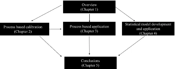
The next three chapters of this dissertation investigate process and statistical approaches to making N management recommendations in two major corn production areas, Iowa (USA) and Central-West Buenos Aires (Argentina, Figure 1.1). I examine the factors controlling the temporal and spatial variability of yields and optimal N rates. By using a long-term experiment from Central Iowa coupled with the APSIM model, I explored how well the cropping system model can simulate crop yield, N dynamics, and economic optimum N rate (EONR). I attempt to answer the question “if the model could predict corn response to N rate, how could this
information be used to develop better N rate guidelines (Chapter 2)?” Next, I assessed the prediction accuracy of a well calibrated crop model as an in-season forecast tool (Chapter 3). In Chapter 4, I developed a new recommendation model for central-west Argentina using
experimental data with advanced statistical techniques. More specifically, I combined dynamic (change rapidly over time, e.g. soil water) and static (fairly stable, e.g. soil organic matter) variables to explore their relative importance on optimal N rate, and used the most important variables to build a statistical model. In the final chapter, I summarized the main findings of this research and offer concluding remarks (Figure 1.1).
Figure 1.1 Thesis diagram
References
Andrade, J. F., & Satorre, E. H. (2015). Single and double crop systems in the Argentine Pampas: Environmental determinants of annual grain yield. Field Crops Research. https://doi.org/10.1016/j.fcr.2015.03.008
Banger, K., Yuan, M., Wang, J., Nafziger, E. D., & Pittelkow, C. M. (2017). A Vision for
Incorporating Environmental Effects into Nitrogen Management Decision Support Tools for U.S. Maize Production. Frontiers in Plant Science. https://doi.org/10.3389/fpls.2017.01270 Basso, B., Sartori, L., Cammarano, D., Fiorentino, C., Grace, P. R., Fountas, S., & Sorensen, C.
a. (2012). Environmental and economic evaluation of N fertilizer rates in a maize crop in Italy: A spatial and temporal analysis using crop models. Biosystems Engineering, 113(2), 103–111. https://doi.org/10.1016/j.biosystemseng.2012.06.012
Batchelor, W. D., Basso, B., & Paz, J. O. (2002). Examples of strategies to analyze spatial and temporal yield variability using crop models. European Journal of Agronomy, 18(1–2), 141–158. https://doi.org/10.1016/S1161-0301(02)00101-6
Berntsen, J., Thomsen, A., Schelde, K., Hansen, O. M., Knudsen, L., Broge, N., … Hørfarter, R. (2006). Algorithms for sensor-based redistribution of nitrogen fertilizer in winter wheat.
Precision Agriculture, 7(2), 65–83. https://doi.org/10.1007/s11119-006-9000-2 Bolsa de Cereales. (2018). Informe ReTAA No7.
Bullock, D. S., Ruffo, M. L., Bullock, D. G., & Bollero, G. A. (2009). The value of variable rate technology: An information-theoretic approach. American Journal of Agricultural
Economics, 91(1), 209–223. https://doi.org/10.1111/j.1467-8276.2008.01157.x
Bundy, L. G., & Adraski, T. W. (1995). Soil yield potential effects on performance of soil nitrate tests. Journal of Production Agriculture, 8, 561–568.
Cassman, K. G., Dobermann, A., & Walters, D. T. (2002). Agroecosystems, nitrogen-use efficiency, and nitrogen management. Ambio, 31(2), 132–140. Retrieved from http://www.ncbi.nlm.nih.gov/pubmed/12078002
Cerrato, M. E., & Blackmer, A. M. (1991). Relationships between leaf nitrogen concentrations and the nitrogen status of corn. Journal of Production Agriculture, 4(4), 525–531.
Ciampitti, I. A., & Vyn, T. J. (2012). Physiological perspectives of changes over time in maize yield dependency on nitrogen uptake and associated nitrogen efficiencies: A review. Field Crops Research, 133, 48–67. https://doi.org/10.1016/j.fcr.2012.03.008
Colaço, A. F., & Bramley, R. G. V. (2018). Do crop sensors promote improved nitrogen management in grain crops? Field Crops Research.
https://doi.org/10.1016/j.fcr.2018.01.007
Davis, D. M., Gowda, P. H., Mulla, D. J., & Randall, A. W. (n.d.). (2000) Modeling Nitrate Nitrogen Leaching in Response to Nitrogen Fertilizer Rate and Tile Drain Depth or Spacing for Southern Minnesota, USA. https://doi.org/10.2134/jeq2000.00472425002900050026x Gleeson, T., Marklund, L., Smith, L., & Manning, A. H. (2011). Classifying the water table at
regional to continental scales. Geophysical Research Letters, 38(5), 1–6. https://doi.org/10.1029/2010GL046427
Gowda, P. H., Mulla, D. J., & Jaynes, D. B. (2008). Simulated long-term nitrogen losses for a midwestern agricultural watershed in the United States. Agricultural Water Management,
95(5), 616–624. https://doi.org/10.1016/j.agwat.2008.01.004
Gregoret, M. C., Dardanelli, J., Bongiovanni, R., & Díaz-Zorita, M. (2006). Modelo de respuesta sitio-específica del maíz al nitrógeno y agua edáfica en un haplustol. Ciencia Del Suelo,
24(2), 147–159.
Kaspar, T. C., Pulido, D. J., Fenton, T. E., Colvin, T. S., Karlen, D. L., Jaynes, D. B., & Meek, D. W. (2004). Relationship of corn and soybean yield to soil and terrain properties.
Agronomy Journal, 96(3), 700–709. https://doi.org/10.2134/agronj2004.0700
Kay, B. D., Mahboubi, a. a., Beauchamp, E. G., & Dharmakeerthi, R. S. (2006). Integrating Soil and Weather Data to Describe Variability in Plant Available Nitrogen. Soil Science Society of America Journal, 70(4), 1210. https://doi.org/10.2136/sssaj2005.0039
Keating, B. A., Carberry, P. S., Hammer, G. L., Probert, M. E., Robertson, M. J., Holzworth, D., … Smith, C. J. (2003). An overview of APSIM, a model designed for farming systems simulation. European Journal of Agronomy, 18(3–4), 267–288.
https://doi.org/10.1016/S1161-0301(02)00108-9
Kersebaum, K. C., Lorenz, K., Reuter, H. I., Schwarz, J., Wegehenkel, M., & Wendroth, O. (2005). Operational use of agro-meteorological data and GIS to derive site specific nitrogen fertilizer recommendations based on the simulation of soil and crop growth processes.
Kersebaum, K. C., Lorenz, K., Reuter, H. I., Wendroth, O., & Ahuja, L. R. (2002). Modelling crop growth and nitrogen dynamics for advisory purposes regarding spatial variability.
Agricultural System Models in Field Research and Technology Transfer. Lewis Publishers, Boca Raton, USA, 229–252.
Kitchen, N. R., Sudduth, K. A., Kremer, R. J., & Myers, D. B. (2010). Sensor-based mapping of soil quality on degraded claypan landscapes of the Central United States. In Proximal Soil Sensing (pp. 363–373). Springer.
Kravchenko, A. N., & Bullock, D. G. (2000). Correlation of corn and soybean grain yield with topography and soil properties. Agronomy Journal, 92(1), 75–83.
https://doi.org/10.1007/s100870050010
Liu, S., Yang, J. Y., Zhang, X. Y., Drury, C. F., Reynolds, W. D., & Hoogenboom, G. (2013). Modelling crop yield, soil water content and soil temperature for a soybean-maize rotation under conventional and conservation tillage systems in Northeast China. Agricultural Water Management, 123, 32–44. https://doi.org/10.1016/j.agwat.2013.03.001
Lory, J. A., & Scharf, P. C. (2003). Yield goal versus delta yield for predicting fertilizer nitrogen need in corn. Agronomy Journal, 95(4), 994–999. https://doi.org/10.2134/agronj2003.0994 Mamo, M., Malzer, G. L., Mulla, D. J., Huggins, D. R., & Strock, J. (2003). Spatial and temporal
variation in economically optimum nitrogen rate for corn. Agronomy Journal, 95(4), 958– 964. https://doi.org/10.2134/agronj2003.9580
Moore, I. D., Gessler, P. E., Nielsen, G. A., & A, P. G. (1993). Moore et al 1993.pdf. Soil Science Society of America Journal, 57, 443–452.
Nangia, V., Turral, H., & Molden, D. (2008). Increasing water productivity with improved N fertilizer management. Irrigation and Drainage Systems, 22(3–4), 193–207.
https://doi.org/10.1007/s10795-008-9051-9
Nosetto, M. D., Jobbágy, E. G., Jackson, R. B., & Sznaider, G. A. (2009). Reciprocal influence of crops and shallow ground water in sandy landscapes of the Inland Pampas. Field Crops Research, 113(2), 138–148. https://doi.org/10.1016/j.fcr.2009.04.016
Orcellet, J., Ignacio, N., Calvo, R., Rene, H., Rozas, S., Wyngaard, N., & Echeverría, H. E. (2017). Anaerobically Incubated Nitrogen Improved Nitrogen Diagnosis in Corn, (May 2016), 1–8. https://doi.org/10.2134/agronj2016.02.0115
Puntel, L. A., Sawyer, J. E., Barker, D. W., Dietzel, R., Poffenbarger, H., Castellano, M. J., … Archontoulis, S. V. (2016). Modeling long-term corn yield response to nitrogen rate and crop rotation. Frontiers in Plant Science, 7(November 2016).
https://doi.org/10.3389/fpls.2016.01630
Quiring, S. M., & Legates, D. R. (2008). Application of CERES-Maize for within-season prediction of rainfed corn yields in Delaware, USA. Agricultural and Forest Meteorology,
Rimski-Korsakov, H., Rubio, G., & Lavado, R. S. (2004). Potential nitrate losses under different agricultural practices in the pampas region, Argentina. Agricultural Water Management. https://doi.org/10.1016/j.agwat.2003.08.003
Rozas, H. S., Echeverría, H. E., Studdert, G. A., & Domínguez, G. (2000). Evaluation of the presidedress soil nitrogen test for no-tillage maize fertilized at planting. Agronomy Journal,
92(6), 1176–1183.
Sawyer, J., Nafziger, E., Randall, G., Bundy, L., Rehm, G., & Joern, B. (2006). Concepts and rationale for regional nitrogen rate guidelines for corn concepts and rationale for regional nitrogen rate guidelines for corn. Iowa State University, University Extension, (April 2006), 1–28.
Scharf, P. C. (2015). Managing nitrogen. Managing Nitrogen in Crop Production, (managingnitroge2), 25–76.
Sela, S., van Es, H. M., Moebius-Clune, B. N., Marjerison, R., Moebius-Clune, D., Schindelbeck, R., … Young, E. (2017). Dynamic Model Improves Agronomic and
Environmental Outcomes for Maize Nitrogen Management over Static Approach. Journal of Environment Quality, 46(2), 311. https://doi.org/10.2134/jeq2016.05.0182
Shahandeh, H., Wright, A. L., & Hons, F. M. (2011). Use of soil nitrogen parameters and texture for spatially-variable nitrogen fertilization. Precision Agriculture, 12(1), 146–163.
https://doi.org/10.1007/s11119-010-9163-8
Sogbedji, J. ., van Es, H. ., Klausner, S. ., Bouldin, D. ., & Cox, W. . (2001). Spatial and temporal processes affecting nitrogen availability at the landscape scale. Soil and Tillage Research, 58(3–4), 233–244. https://doi.org/10.1016/S0167-1987(00)00171-9
Stanford, G., Legg, J., & Smith, S. (1973). Soil nitrogen availability evaluations based on nitrogen mineralization potentials of soils and uptake of labeled and unlabeled nitrogen by plants. An International Journal on Plant-Soil Relationships, 39(1), 113–124.
https://doi.org/10.1007/BF00018050
Thompson, L. J., Ferguson, R. B., Kitchen, N., Frazen, D. W., Mamo, M., Yang, H., & Schepers, J. S. (2015a). Model and sensor-based recommendation approaches for in-season nitrogen management in corn. Agronomy Journal, 107(6), 2020–2030.
https://doi.org/10.2134/agronj15.0116
Thompson, L. J., Ferguson, R. B., Kitchen, N., Frazen, D. W., Mamo, M., Yang, H., & Schepers, J. S. (2015b). Model and Sensor-Based Recommendation Approaches for In-Season
Nitrogen Management in Corn. Agronomy Journal, 0(0), 0. https://doi.org/10.2134/agronj15.0116
Thorp, K. R., Malone, R. W., & Jaynes, D. B. (2007). Simulating long-term effects of nitrogen fertilizer application rates on corn yield and nitrogen dynamics. Transactions of the ASABE,
Van Ittersum, M. K., Leffelaar, P. A., Van Keulen, H., Kropff, M. J., Bastiaans, L., & Goudriaan, J. (2002). Developments in modelling crop growth, cropping systems and production systems in the Wageningen school. NJAS - Wageningen Journal of Life Sciences, 50(2), 239–247. https://doi.org/10.1016/S1573-5214(03)80009-X
Vanotti, M. B., & Bundy, L. G. (1994a). An alternative rationale for corn nitrogen fertilizer recommendations. Journal of Production Agriculture, 7(2), 243–249.
https://doi.org/10.2134/jpa1994.0243
Vanotti, M. B., & Bundy, L. G. (1994b). Corn Nitrogen Recommendations Based on Yield Response Data. Journal of Production Agriculture, 7(2), 249.
https://doi.org/10.2134/jpa1994.0249
Yang, J. M., Yang, J. Y., Liu, S., & Hoogenboom, G. (2014). An evaluation of the statistical methods for testing the performance of crop models with observed data. Agricultural Systems, 127, 81–89. https://doi.org/10.1016/j.agsy.2014.01.008
CHAPTER 2. MODELING LONG-TERM CORN YIELD RESPONSE TO NITROGEN RATE AND CROP ROTATION
Modified from a paper published in Frontiers in Plant Science, November 2016 |
https://doi.org/10.3389/fpls.2016.01630
Laila A. Puntel1, John E. Sawyer1, Daniel W. Barker1, Ranae Dietzel1, Hanna Poffenbarger1, Michael J. Castellano1, Kenneth J. Moore1, Peter Thorburn2 and Sotirios V. Archontoulis1
1Department of Agronomy, Iowa State University, Ames, IA, USA
2Commonwealth Scientific and Industrial Research Organisation Agriculture, St Lucia,
QLD, Australia
Abstract
Improved prediction of optimal N fertilizer rates for corn (Zea mays L.) can reduce N losses and increase profits. We tested the ability of the Agricultural Production Systems sIMulator (APSIM) to simulate corn and soybean (Glycine max L.) yields, the economic optimum N rate (EONR) using a 16-year field-experiment dataset from central Iowa, USA that included two crop sequences (continuous corn and soybean-corn) and five N fertilizer rates (0, 67, 134, 201, and 268 kg N ha-1) applied to corn. Our objectives were to: (a) quantify model
prediction accuracy before and after calibration, and report calibration steps; (b) compare crop model-based techniques in estimating optimal N rate for corn; and (c) utilize the calibrated model to explain factors causing year to year variability in yield and optimal N. Results indicated that the model simulated well long-term crop yields response to N (relative root mean square error, RRMSE of 19.6% before and 12.3% after calibration), which provided strong evidence that important soil and crop processes were accounted for in the model. The prediction of EONR was more complex and had greater uncertainty than the prediction of crop yield (RRMSE of
44.5% before and 36.6% after calibration). For long-term site mean EONR predictions, both calibrated and uncalibrated versions can be used as the 16-year mean differences in EONR’s were within the historical N rate error range (40–50 kg N ha-1). However, for accurate year-by-year simulation of EONR the calibrated version should be used. Model analysis revealed that higher EONR values in years with above normal spring precipitation were caused by an exponential increase in N loss (denitrification and leaching) with precipitation. We concluded that long-term experimental data were valuable in testing and refining APSIM predictions. The model can be used as a tool to assist N management guidelines in the US Midwest and we identified five avenues on how the model can add value toward agronomic, economic, and environmental sustainability.
Introduction
The economic optimum nitrogen (N) rate (EONR) is the fertilizer rate at which crop yield increase is not large enough to pay for additional N application, and therefore more N would only result in unnecessary costs (Sawyer et al., 2006). Optimal N input needs to be considered when making N recommendations since it has the potential to improve N use efficiency, crop yield, and profitability as well as to reduce environmental impacts (Wang et al., 2003; Lawlor et al., 2008; Kyveryga et al., 2009; Basso et al., 2016). Nitrogen losses by leaching are proportional to the N rate applied and tend to increase rapidly at rates greater than optimal for crop use
(Haghiri et al., 1978; Cooper and Cooke, 1984; Andraski et al., 2000; Randall et al., 2000). There is tremendous uncertainty and risk associated with prediction of the EONR in corn–based systems, both at the field and sub-field scale (Paz et al., 1999; Scharf et al., 2005; Tremblay et al., 2012). Farmers may attempt to protect corn yield potential with high fertilizer N inputs, which leads to decreased profitability (Lambert et al., 2006) and increased likelihood of
environmental contamination (Andraski et al., 2000; Jaynes et al., 2001; Robertson and Groffman, 2007).
A number of approaches have been developed to predict optimal N application rates. These include yield goal-based N recommendations and N budgets (Stanford, 1973, 1982; Stanford and Legg, 1984), pre-plant and pre-sidedress soil nitrate test (PPNT and PSNT, Bundy and Andraski, 1995; Shapiro et al., 2008), Illinois soil nitrogen test (ISNT, Mulvaney et al., 2001), crop canopy sensing (NDVI, Schmidt et al., 2009 and chlorophyll meter, Blackmer and Schepers, 1995; Varvel et al., 1997), and economic maximum return to N (MRTN, Sawyer et al., 2006). Some of these tools are static in that they give the same recommendation regardless of yearly weather or crop/fertilizer prices, or evaluate N status after grain crop harvest. Soil tests or hand-held crop meters are often time consuming, expensive, and/or require periodic and intense sampling (Blackmer et al., 1997; Ma and Dwyer, 1999; Grove and Schwab, 2006; van Es et al., 2007; Lemaire et al., 2008; Franzen et al., 2016). Most current and widely adopted N
management practices also assume field-uniformity, recommending N applications that ignore variation in landscape factors such as topography, soil texture, and organic matter (Cassman et al., 2002; Mamo et al., 2003; Scharf et al., 2005), as well as interactions with plant population and hybrid (Ciampitti and Vyn, 2012). Use of precision agriculture technologies (real-time remote sensing, unmanned aerial images, soil mapping, etc.) combined with variable N application have the potential to increase N use efficiency by matching the N requirements within field zones (Dobermann and Cassman, 2002; Ferguson et al., 2002; Mamo et al., 2003; Mulla, 2013). However, the selection of a site-specific optimum N rate is difficult to predict based on the large temporal and spatial variability of the N supply and demand (van Es et al., 2007; Setiyono et al., 2011). Unfortunately, the above approaches have not fully resolved needed
improvements from N management and gains in N use efficiency (Raun and Johnson, 1999; Fageria and Baligar, 2005) since N losses from corn-based systems are still high with negative environment impacts (Jaynes et al., 2001; Mitsch et al., 2001).
The challenge in managing N and estimating the optimum N fertilization rate comes from the complex interactions that exist in the dynamic soil-plant-atmosphere system and uncertainty in weather (Havlin et al., 2005; Tremblay and Belec, 2006; Brady and Weil, 2008). Soil N mineralization from SOC and crop N uptake, and N losses are three important components defining the optimum N rate, however, these processes are dynamic and difficult to predict (Cassman et al., 2002). Therefore N management tools that simultaneously consider dynamics in soil organic carbon mineralization, crop growth, weather conditions, and agronomic practices may greatly improve site- and year-specific EONR estimates (Basso et al., 2012, 2016; Dumont et al., 2016). Dynamic cropping system simulation models such as Agricultural Production Systems sIMulator (APSIM; Holzworth et al., 2014), DSSAT (Jones et al., 2003), RZWQM (Ahuja et al., 2000), CropSyst (Stockle et al., 2003), SALUS (Basso et al., 2006), and others have been used to investigate soil-crop-weather dynamics, however, model use has been limited to address long-term optimum N rates (Ma et al., 2007; Basso et al., 2010). The scientific literature is also rich with examples of model applications to improve our understanding of N dynamics and to answer questions that cannot be addressed with field research due to time and cost constraints (Batchelor et al., 2002; Schnebelen et al., 2004; Fountas et al., 2006; Malone et al., 2010; Basso et al., 2012, 2016; Anapalli et al., 2014). However, use of models in practical applications to assist real-life challenges such as N rate guidance is limited because models typically require: (a) a large number of input parameters, which are usually not available
(Wallach, 2006; Basso et al., 2012); (b) particular skills to develop model specific input parameters and cultivar coefficients from internet databases; and (c) intensive training for use.
Over the last few years web-applications have been developed to simplify the use of models (e.g., Yield Prophet, Carberry et al., 2009). Furthermore, digital soil and weather
databases such as web soil survey1 (Soil Survey Staff, 2006) and daymet (Daymet, 1980–2008; Thornton et al., 2012) provide free access to high-resolution input parameters. As a result, the potential of using simulation models to assist with real-life practical problems and especially to predict the risk associated with selecting specific N fertilizer rates has received strong industrial interest (Thorp et al., 2007; Gowda et al., 2008; Nangia et al., 2008). The next challenge to applying models across different scales (within fields, regions, and cropping systems) is to determine prediction accuracy; e.g., how well cropping system models can predict crop yield, N dynamics, and EONR. And if they can predict corn response to N rate, how can this information be used to develop better N rate guidelines.
In this study we used a 16-year field research dataset from a site in central Iowa, USA that included five N rates and two crop sequences to test the ability of the APSIM model (Holzworth et al., 2014) to predict crop yields and optimal N rate for corn.
Objectives
Our specific objectives were to: (a) quantify model prediction accuracy before and after calibration, and report calibration steps; (b) compare crop model-based techniques in estimating optimal N rate for corn; and (c) utilize the calibrated model to explain factors causing year to year variability in yield and optimal N.
Materials and Methods Site, Weather, and Experimental Datasets
The field-experiment was conducted at the Agricultural Engineering and Agronomy Research Farm near Ames, Iowa, USA (42° 0′37.50″N, 93°47′22.98″W) on a Clarion loam soil (fine-loamy, mixed, superactive, mesic Typic Hapludoll). The experiment was initiated in 1999 and continuous to the present. For this study we used data from 1999 to 2014 (16-years). The climate at the site is humid continental (warm, rainy summers) with annual precipitation of 900 mm and a mean temperature of 9°C (Supplementary Figure S1). Over the 16-year experimental period, crops experienced warm and wet conditions (3 years), cool and wet conditions (3 years), warm and dry conditions (5 years), and cool and dry conditions (5 years; Supplementary Figure S1). Years 2008, 2010, and 2014 were the wettest and years 2000, 2011, 2012, and 2013 the driest. Mean annual air temperatures were 16 and 23°C for spring and summer, respectively. Year 2012 was the warmest and year 2008 the coolest (Supplementary Figure S1).
The long-term experiment was designed to study the effect of five N fertilizer rates (0, 67, 134, 201, and 268 kg N ha-1; hereafter N0, N67, N134, N201, and N268, respectively) on corn yield in continuous corn (CC) and soybean-corn rotation (SC). The experimental design was a randomized complete block design with four replications. Nitrogen fertilizer was applied near planting (± 10–15 days). Specific information on the fertilizer type and application dates are provided in Supplementary Table S1. Within the SC rotation, corn and soybean phases were present each year in the rotation: thus a simulation starting with corn in year one and another simulation starting with soybeans on year one were set up. Hereafter SC when the rotation starts with corn in year one (odd numbered years) and a validation set (SC_val) when the rotation starts with soybean in year 1 (even numbered years). Each treatment had four replications. Nitrogen fertilizer was only applied to corn. Supplementary Table S1 provides management information
by year and rotation. Measurements included corn and soybean grain yields each year (expressed at 15.5 and 13% moisture content, respectively). Soil organic carbon measurements were
available at 0–15 cm in 1999, 2009, and 2014, and at 0–30 cm in 2009 for CC (Brown et al., 2014; Poffenbarger et al., unpublished).
The APSIM Modeling Platform
The APSIM (Keating et al., 2003; Holzworth et al., 2014) is an open-source advanced simulator of agricultural systems that combines several process-based models in a modular design. APSIM is a field-scale model that operates mainly on a daily time step. The APSIM model was selected for use in this study because of its flexibility and easy use in specifying crop rotations via the user interface, capability in simulating long-term dynamics in both soil and crop processes, advanced flexibility in simulating the effect of shallow water table dynamics that are important in this geographic region (Helmers et al., 2012) and previously determined good performance in this geographic region (Malone et al., 2007; Hammer et al., 2009; Lobell et al., 2013; Archontoulis et al., 2014a,b, 2016; Basche et al., 2016; Dietzel et al., 2016; Martinez-Feria et al., 2016). Details about APSIM and its performance across a range of studies can be found at http://www.apsim.info.
APSIM Configuration and Calibration
Two rounds of APSIM model evaluations were performed; a blind phase (uncalibrated model) where management and cultivar information were used, and a calibrated phase
(calibrated model) where crop yield and SOC data were provided into the model. Similar protocols have been used in the AgMIP project (Agricultural Model Inter-Comparison and Improvement Project; Rosenzweig et al., 2013).
Blind-Phase Model Parameters and Set-Up
For the blind phase, we first incorporated available management information into APSIM (Supplementary Table S1). When required management information was unavailable, we used typical values from the literature relevant to the research site (Abendroth et al., 2011; Pedersen and Licht, 2014). The following input parameters were held constant across the 16-years: planting depth of 5 cm for both crops, plant populations of 8 and 38 plants m-2 for corn and soybean, respectively, and November 10th and April 10th dates for fall and spring tillage operations; and corn hybrid (106-day) and soybean variety (2.5 maturity group) values derived from previous studies in the region (Archontoulis et al., 2014a,b; Supplementary Table S2). Daily weather data were obtained from the Iowa Environmental Mesonet (2014). Soil profile information was taken from Web Soil Survey (Soil Survey Staff, 2006) and soil-root related parameters were developed following the methodology described in Archontoulis et al. (2014a). The maximum rooting depths for corn and soybean were set to 1.5 and 1.2 m, respectively.
We set up APSIM by connecting the following models: corn and soybean crop models (Keating et al., 2003), Soil N (soil N and C cycling model with default soil temperature model; Probert et al., 1998), SoilWat (a tipping bucket soil water model; Probert et al., 1998);
SURFACEOM (residue model; Probert et al., 1998; Thorburn et al., 2001, 2005), and the
following management rules: planting, harvesting, fertilizer, tillage, and rotations (Keating et al., 2003). In addition we implemented within the MANAGER module an N deposition rule that simulates atmospheric N deposition as a function of daily precipitation (N deposition in kg N ha
-1 d-1 = 0.01∗ precipitation in mm; Holland et al., 2005). On average, this added about 7 kg N ha-1
year-1 into the system. Initial model conditions such as root mass, surface residue mass, soil
water, soil nitrate, and SOC pool partitioning were obtained by starting the model 6 years prior to the start of the experiment (Supplementary Table S3). Experience using APSIM in this
geographic region for simulating corn-soybean production systems has indicated that the fast microbial SOC pool (BIOM) of APSIM requires at least 4 years to stabilize (Basche et al., 2016; Dietzel et al., 2016; Martinez-Feria et al., 2016). Having this pool stabilized is important to remove confounding effects of microbial SOC buildup or decline which affects N dynamics. The APSIM version 7.6 was used on a daily time step. The simulation process was consecutive to account for carry-over effects from year to year, such as soil inorganic nitrogen, soil moisture, root and residue carbon and nitrogen inputs from previous crops.
Model Calibration and Testing
In the calibration and testing phase, we used end-of-season grain yields and SOC data to improve predictions. The long-term (end-of-season) data are powerful in detecting weakness in the model (i.e., years with low prediction accuracy), but do not provide guidance on which of the model’s processes or parameters needed to be improved. Therefore, to inform the calibration process, additional information was used: knowledge gained from other APSIM calibration studies in Iowa (Archontoulis et al., 2014a, 2016; Basche et al., 2016; Dietzel et al., 2016), sensitivity techniques, and model behavior analysis coupled with expert judgment
(Supplementary Figure S2). The odd-numbered years (for CC and SC) were used for calibration and even numbered years for validation (SC_val dataset).
During calibration the following changes in APSIM were made: first, we replaced the default APSIM soil temperature model that uses EPIC model equations (Williams et al., 1984) with a more mechanistic soil temperature model (Campbell, 1985) available in APSIM
(soiltemp2). The reason was twofold: (a) soiltemp2 has been found to perform better in Iowa (Archontoulis et al., 2014a; Basche et al., 2016; Dietzel et al., 2016); and (b) soiltemp2 better represents reality than the default model as it accounts for soil temperature changes due to tillage, residue cover, and management practices. Second, we replaced SoilWat with the SWIM
soil water model (Huth et al., 2012) available in APSIM. This model allowed simulation of fluctuating shallow groundwater tables, which in this region varies from about 80 to 200 cm (Groundwater, USGS, Iowa Water Science Center). Third, we improved the simulation of soybean residue C:N ratio at harvest because the simulated C:N ratio was low when compared to published data (Johnson et al., 2007) and caused an over-prediction of corn yields in the SC rotation with no N applied. We improved soybean C:N ratio by decreasing the critical N concentration of different plant tissues at physiological maturity by about 20% (Supplementary Table S2). Additionally, we decreased the potential N fixation rate (Supplementary Table S2) to better match seasonal N fixation estimates to those observed in the literature for this region (Salvagiotti et al., 2008). No changes were made in the corn crop model, although various options were explored via sensitivity analysis. Given all these changes we re-initialized conditions at the start of the simulation on year 1999 (Supplementary Table S3). Data Analysis
Estimation of the Annual Economic Optimum Nitrogen Rate
The relationship between observed or simulated yield and N rate was fit using the quadratic
Equation 1 y=a+bx+cx2 or the quadratic-plus-plateau,
Equation 2 y=a+bx+cx2, x<x0
Equation 3 y=a+bx0+cx20, x≥x0
In these equations, y represents corn yield (either observed or simulated), x is the
fertilizer N rate, a is the intercept, b is the linear coefficient, c is the quadratic coefficient, and x0 is the N rate at the join point. The PROC NLIN procedure in SAS (Version 9.4, SAS, 2013).
Equations were deemed significant at p < 0.05 and the equations with the smallest sums of squares and largest R2 were selected.
Corn EONR and the yield at the EONR (YEONR) were calculated from the N response equations by setting the first derivative of the fitted response curve equal to the historical price ratio of 5.6:1 N:corn grain price (US$ kg-1 N:US$kg-1 grain) ratio (Cerrato and Blackmer, 1990; Bullock and Bullock, 1994). The impact of the N:corn grain price ratio on EONR has been well documented in the literature (Cerrato and Blackmer, 1990; Sawyer et al., 2006). In this study, we used a fixed ratio across years similarly to other modeling studies (Basso et al., 2012). Using this approach, we calculated EONR and YEONR values for: (a) the observed data (EONR-Obs, YEONR-Obs); (b) the simulated data from the uncalibrated model (EONR-APSIM-Unc, YEONR-APSIM-Unc); and (c) the simulated data from the calibrated model (EONR-APSIM-Cal, YEONR-Cal).
Additionally, a different technique to calculate an optimal N rate was used (Basso et al., 2016). The calibrated APSIM model was ran for every 5 kg N ha-1 increments from 0 to 350 kg N ha-1 to simulate corn yields. Then the N rate at which the economic return on N was
maximized [hereafter RTN (return to N approach)-APSIM] was estimated by difference: simulated yield times corn price minus fertilizer rate times N cost between two levels of N rate. A value of zero (or near zero) corresponds to the optimum N rate. Same prices for corn grain and N fertilizer was used as with the EONR technique.
The RTN-APSIM technique differs from the EONR-APSIM-Cal in the following way: EONR-APSIM-Cal estimates the economic optimum N rate through regression equations (Equation 1-3) fitted to five simulated corn yields at 0, 68, 134, 200, and 268 kg N ha-1. The
yield (every 5 kg N, from 0 to 350 kg N ha-1) and therefore the economic optimum N rate can be identified without use of regression equations. The RTN approach follows a similar methodology to that is currently used for corn N rate recommendations in the USA Midwest (known as the MRTN approach; Sawyer et al., 2006). The difference between RTN-APSIM and MRTN is that the regression equations for MRTN are within a database with extensive N rate response trials and associated regression equations, while RTN-APSIM generates a synthetic database, which depends on the accuracy of the model to predict yields and N response.
Estimation of Site Mean Economic Optimum Nitrogen Rate
Two methods were used to estimate the site mean EONR and YEONR: (a) we first averaged individual annual estimates of EONR and YEONR for each rotation, and then
calculated the associated standard deviation (SD; across years mean); and (b) we averaged corn yields across years for each rotation and then we estimated EONR and YEONR using regression equation fitting and EONR calculation, which is an approach used for N recommendations (pooled mean, Sawyer et al., 2006). The same methods were used for RTN-APSIM, except no regression equation fitting was required.
Statistical Evaluation of Model Performance
To evaluate APSIM model goodness of fit, we used graphical and statistical methods. For the statistical evaluation, we computed the root mean square error (RMSE),
Equation 4 RMSE=√∑ (𝑆𝑖−𝑂𝑖)2
𝑛 𝑖=1
𝑛 and RRMSE,
Equation 5 RRMSE= 𝑅𝑀𝑆𝐸
𝑂̅ x 100
where Ō is the mean observed value, Si is the model estimated value, Oi is the observed value, and n is the number of data pairs. The RMSE summarizes the average difference between observed and predicted values, while RRMSE provides the relative difference. In both cases, the lower the value of the index the better the model performance. In this study, we considered RRMSE ≤ 15% as “good” agreement; 15–30% as “moderate” agreement; and ≥ 30% as “poor” agreement (Liu et al., 2013; Yang et al., 2014).
Factors Affecting Optimal Nitrogen Rate Inter-Annual Variability
Regression analysis was performed to identify statistical significant relationships between simulated EONR and explanatory factors. We considered three explanatory factors: yield at optimum N rate, time of N application rate relative to corn planting date, and precipitation sums over different time periods. We used R2 to evaluate predictability of optimum N rate based on the factors mentioned above.
Results
Observed Corn and Soybean Yield Response to N Fertilizer, and Crop Rotation
Observed corn yield varied across years, N rates, and crop sequences (Figure 2.1, Figure 2.2). Yearly variability CC, corn yield averages across years ranged from 4.2 (N0) to 11.6
(N268) Mg ha-1 with a maximum yield response to N (difference between N0 and N268 treatment) of 7.6 Mg ha-1 (Figure 2.3). In SC, corn yield averages were greater for all N
treatments compared to CC, and varied from 7.8 (N0) to 12.9 (N268) Mg ha-1 with a maximum yield response to N of 5.1 Mg ha-1. At N0, for individual years the largest yield difference
between CC and SC was 3.6 Mg ha-1. Greater yearly variability in corn yield was observed in CC
(coefficient of variation, CV = 17.8%) than in SC (CV = 12.9%). The CV decreased with increasing N rate in CC (from 24.8 to 15.4%), but was consistent across N rate in SC. Across
rotations, high corn yields under non-limited N condition were obtained in wet years
(precipitation above 1100 mm, e.g., 2008 and 2010; Figure 2.1, Figure 2.2, Figure 2.3) and low corn yields in dry years (precipitation below 600 mm precipitation, e.g., 2000, 2012, and 2013). Observed soybean yields varied from 2.1 to 4.8 Mg ha-1 across years and N rates (Figure 2.4; Supplementary Figure S2). The yearly variability in soybean yield had a CV of 19.5%. Soybean yields were not affected by N rates applied to corn (Figure 2.3; Supplementary Figure S2). Model Accuracy before and after Calibration
Simulation of Corn Yields
Overall, across years, N rates and crop sequences, APSIM explained from 50–69% (before calibration) to 67–88% (after calibration) of the observed variability in corn yield (Figure 2.3). The model agreement improved during calibration from moderate (RRMSE = 19.6%,
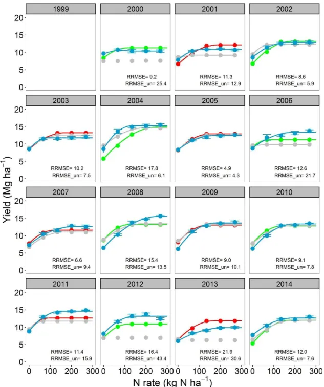
uncalibrated) to good (RRMSE = 12.3%, calibrated) for corn yield prediction (Figure 3). In CC, the uncalibrated model simulated corn yield response to N well in 7 years (RRMSE < 15%), moderately well in 6 years (RRMSE 15–30%), and poorly in 3 years (RRMSE > 30%); while after calibration the model simulated yields well in 14 years and moderately well in 3 years (Figure 2.1).
In SC, the uncalibrated model simulated corn yield response to N well in 10 years, moderately well in 3 years, and poorly in 2 years; while after calibration the model simulated yields well in 11 years and poorly in 4 years (Figure 2.2). In general the calibrated model captured the trends in the observed variability in corn yields across years (Supplementary Figure S4A) as well as the annual yield response to N rates (Figure 2.1 and Figure 2.2).
Figure 2.1 Corn yield response to N fertilizer for the continuous corn (CC) cropping system. The blue points with standard errors (n = 4) indicate the observations. The gray and red points are Agricultural Production Systems sIMulator (APSIM) simulations before and after calibration, respectively. Continuous lines are regression fits from Eqs. 1–3. When lines are not shown it means that Eqs. 1–3 did not converge. Relative root mean square error for both calibrated (RRMSE) and uncalibrated model (RRMSE_un) are shown for each year.
Figure 2.2 Corn yield response to N fertilizer for the soybean-corn (SC) cropping system. The blue points with standard errors (n = 4) indicate the observations. The gray, red, and green points indicate uncalibrated, calibrated and validated simulations from the Agricultural Production Systems sIMulator (APSIM) model. Continuous lines are regression fits from Eqs. 1–3. When lines are not shown it means that Eqs. 1–3 did not converge. Relative root mean square error for both calibrated (RRMSE) and uncalibrated model (RRMSE_un) are shown for each year.
Figure 2.3 Sixteen year mean crop yield response to N fertilizer rate (A, D, and G panels), and observed versus simulated crop yields across years and N rate (B, C, E, F, H, and I). Points are observations or simulations, continuous lines are regression fits from Eqs. 1–3, and broken lines show 1:1 relationship.
Figure 2.4 Economic optimum N rate (EONR) and corn yield at the EONR (YEONR) for every year in CC and SC. The EONR and YEONR estimates from observations using Eqs. 1-3 are shown as bars. Different color symbols show Agricultural Production Systems sIMulator (APSIM) model simulations: red points calibrated model, gray points uncalibrated model, and green points return to N approach (RTN) from the calibrated model.
Simulation of Soybean Yields
Given that the simulation setup was sequential and soybean was part of the CS rotation, the ability of APSIM in simulating soybean yields was also tested. The model simulated no response to N rate applied to the previous corn crop, which agrees with the observed data (Figure 4; for individual years see Supplementary Figure S3). The agreement in simulated soybean yields was moderate before and after calibration (calibrated RRMSE = 19%; Figure 2.3).
Simulation of Optimum N Rate and Methods Comparison Site Mean Optimum N Rate
The calibration process improved the prediction of the site mean EONR in the SC but not in CC (Table 2.1; Figure 2.3 Sixteen year mean crop yield response to N fertilizer rate (A, D, and G panels), and observed versus simulated crop yields across years and N rate (B, C, E, F, H, and I). Points are observations or simulations, continuous lines are regression fits from Eqs. 1–3, and broken lines show 1:1 relationship.). The simulated EONR (both calibrated and uncalibrated versions) was overestimated in CC and underestimated in SC (Table 2.1). The absolute
difference in site mean EONR between simulated and observed values was smaller in SC; -39 and 18 kg N ha-1 for CC and SC, respectively, before calibration and -41 and 10 kg N ha-1 for CC and SC, respectively, after calibration (Table 2.1). In addition, the simulated EONR SD was high with the APSIM-Unc, largely due to mis-estimation of some years as non-N responsive.
Table 2.1 Mean economic optimum N rate (EONR, kg N ha-1) across 16-years for: observed,
Obs; un-calibrated Agricultural Production Systems sIMulator (APSIM) model, Unc; calibrated model, Cal; and the return to N approach from the calibrated model, RTN.
12
1 Individual annual optimum N rate estimates were averaged across 16-years and the standard deviation (SD) calculated
2 Individual annual corn yield values were first averaged across years and then the optimum N rates estimated
Obs Unc Cal RTN Obs-Unc Obs-Cal Obs-RTN
Rotation Mean values Differences
Average of years ± SD1 CC 188 ± 42 190 ± 82 225 ± 33 176 ± 21 -2 -37 12 SC 149 ± 48 99 ± 71 137 ± 43 118 ± 30 50 12 31 Pooled2 CC 187 226 228 195 -39 -41 -8 SC 158 140 147 140 18 10 18
Annual Optimum N Rate
The calculated EONR-Obs (from observations) was highly variable from year to year and ranged from 123 to 268 kg N ha-1 in CC and from 42 to 241 kg N ha-1 in SC (Figure 2.4). The inter-annual variability in EONR-Obs was greater in SC than in CC (CV of 32 vs. 22%, respectively).
The calculated EONR from the APSIM model followed some of the observed annual trends (Figure 2.4), with the prediction error to be larger in SC than CC (Supplementary Figure S7). In CC, the RMSE ranged from 63 kg N ha-1 before calibration to 56 kg N ha-1 after
calibration. In SC, the RMSE ranged from 83 kg N ha-1 before calibration to 68 kg N ha-1 after
calibration. Interestingly, the two methods of calculating EONR from modeled yields (via regression Eqs. 1–3 or via the RTN approach) had similar RMSE and RRMSE values across years, but the annual predictions of optimum N using the RTN approach were less variable across years (Figure 2.4). These results show that for year-to-year simulation of EONR, the calibrated version should be used either via Eqs. 1–3 with regression analysis or the RTN approach. Overall the calibration process reduced the RRMSE in annual EONR predictions by 14.2% in CC and 10.3% in SC (Supplementary Figure S8).
The calculated yearly YEONR-Obs (from observation) was less variable compared to the EONR variability (CV of 17 and 12% for CC and SC, respectively, Figure 2.4). The simulated YEONR followed the observed annual trends well (Figure 4; RMSE of 1.88 Mg ha-1 before calibration and 1.41 Mg ha-1 after calibration). The model simulated YEONR was more accurate than EONR. In relative terms, the error in YEONR prediction was about four times lower than the error in EONR prediction (Supplementary Figures S6 and S7). However, there was no correlation between these errors (Supplementary Figure S6).
Use of the RTN approach to compute the optimum N rate, and compared to the simulated calibrated values (Table 2.1), produced a closer EONR in CC to the observed EONR (-8 kg N ha-1), but a greater difference in SC (18 kg N ha-1). Unlike the APSIM-Cal and APSIM-Unc simulations, the RTN-APSIM did not over-estimate EONR in CC, but underestimated in SC (Table 2.1).
Factors Causing Yearly Variability in Optimal Nitrogen Rate
The YEONR-Obs (Supplementary Figure S5), precipitation (Figure 2.5), and the time of N application (Supplementary Figure S8) were explored as possible factors to explain inter-annual variability in EONR. There was a significant positive relationship between spring
precipitation and EONR-Obs but the relationship had low predictive power (p < 0.05; R2 = 0.27– 0.45; Figure 2.5). Spring precipitation, defined here as precipitation accumulated from April 1 to June 31, was selected from among many other precipitation intervals explored in this study as the best predictor of inter-annual EONR variability (Supplementary Figure S8). The YEONR, time of N rate application, the July precipitation (15 days window around corn silking), and
combinations of those factors (including spring precipitation) via multi-factor regression modeling did not result in any significant correlation.
Figure 2.5 Cumulative spring precipitation from April 1st to June 30th (every year) versus economic optimum N rate (observed and simulated EONR, circles and squares, respectively; top panels), simulated spring soil N supply (from soil organic carbon mineralization; middle panels), and simulated spring N loss (denitrification and leaching; lower panels) for CC and SC crop sequences.
The calibrated APSIM version showed a similar relationship between EONR and spring precipitation as with EONR-Obs (Figure 2.5) and therefore the model was used to provide insights into factors causing this relationship. Soil net N mineralization (simulated N supply), and the sum of denitrification and N leaching below 1 m depth (simulated N loss) were used as explanatory variables. The model indicated that the relationship between EONR and spring precipitation was primarily caused by an exponential increase in simulated N loss and to some
extent by a reduction in simulated N supply with increasing spring precipitation (Figure 2.5). The model also showed that the rate of the simulated N supply reduction with increased
precipitation was similar between rotations. Furthermore model analysis showed that the level of simulated N supply was 50% higher in SC than CC, which explains the lower EONR values typically found in SC systems (Figure 2.3).
Discussion Calibration Strategy and Steps
Evaluating a model against long-term data is critical when the model is to be used for N management. This is because processes such as N mineralization, require several years to be sufficiently evaluated (Jenkinson et al., 1994; Leigh et al., 1994; Körschens, 2006) and can differentially affect N response among years. Our study is among a few in the literature that tests a process-based model in the long-term (Ma et al., 2007). The long-term data were powerful in detecting weakness in the model, but did not provide guidance on which of the model’s
processes or parameters needed to be improved (Kersebaum et al., 2015). Therefore, during calibration we aimed to improve the overall representation of the system based on previous knowledge of the site (for example, C:N ratio of soybean and corn residue, phenology, etc.) rather than just optimizing cultivar parameters by year to better fit the observed data within the study range. This strategy is robust and allows the calibrated model to be used outside the study period (future years) with confidence at this site.
During calibration we implemented the alternate soil water (SWIM) and temperature (soiltemp) models available in the framework, and changed parameters influencing soybean residue C:N ratio (Table 2.2; Figure 2.3). Among changes made in the model, the activation of fluctuating water table via the SWIM soil water model was found to be the most important (e.g., see improvements in yield prediction from 2012 drought in Figure 2.2 and Figure 2.3). Yet, few