NBER WORKING PAPER SERIES
CAPM OVER THE LONG RUN: 1926-2001 Andrew Ang
Joseph Chen Working Paper 11903
http://www.nber.org/papers/w11903
NATIONAL BUREAU OF ECONOMIC RESEARCH 1050 Massachusetts Avenue
Cambridge, MA 02138 December 2005
The authors especially thank Geert Bekaert, Mikhail Chernov, Ethan Chiang, Frank Diebold, Ken French, Yufeng Han, Jonathan Lewellen, Stefan Nagel, ZhenyuWang, and Guofu Zhou for very detailed comments. We also thank Ilan Cooper, Wayne Ferson, Cam Harvey, Bob Hodrick, Michael Johannes, Craig MacKinlay, an anonymous referee, and seminar participants at Columbia University, Duke University, INSEAD, SAC Capital Management, UCLA, UC Riverside, University of Alabama, USC, Wharton, the American Finance Association, the Econometric Society Annual Meeting, the Econometric Society World Congress, a Q-Group meeting, the Simulation-Based and Finite Sample Inference in Finance Conference at Quebec City, and the Western Finance Association. We are grateful to Ken French for making his data available. The views expressed herein are those of the author(s) and do not necessarily reflect the views of the National Bureau of Economic Research.
©2005 by Andrew Ang and Joseph Chen. All rights reserved. Short sections of text, not to exceed two paragraphs, may be quoted without explicit permission provided that full credit, including © notice, is given
CAPM Over the Long Run: 1926-2001 Andrew Ang and Joseph Chen
NBER Working Paper No. 11903 December 2005
JEL No. C51, G12
ABSTRACT
A conditional one-factor model can account for the spread in the average returns of portfolios sorted by book-to-market ratios over the long run from 1926-2001. In contrast, earlier studies document strong evidence of a book-to-market effect using OLS regressions in the post-1963 sample. However, the betas of portfolios sorted by book-to-market ratios vary over time and in the presence of time-varying factor loadings, OLS inference produces inconsistent estimates of conditional alphas and betas. We show that under a conditional CAPM with time-varying betas, predictable market risk premia, and stochastic systematic volatility, there is little evidence that the conditional alpha for a book-to-market trading strategy is statistically different from zero.
Andrew Ang
Columbia Business School 3022 Broadway 805 Uris New York NY 10027 and NBER
[email protected] Joseph Chen
University of Southern California [email protected]
1
Introduction
Beginning with Basu (1983), many researchers have found significant evidence over the post-1963 period of a book-to-market effect, where stocks with high book-to-market ratios have higher average returns than what the CAPM predicts. This inference is based on conventional OLS with asymptotic standard errors, which relies on the assumptions that factor loadings are constant and that the market risk premium is stable. However, both of these assumptions are violated in data. In particular, betas of book-to-market portfolios vary substantially over time. For example, betas of the highest decile of book-to-market stocks reach over 3.0 prior to 1940 and fall to -0.5 at the end of 2001 (see also Kothari, Shanken and Sloan, 1995; Campbell and Vuolteenaho, 2004; Adrian and Franzoni, 2005).
After taking into account time-varying betas and market risk premia, we find that the con-ditional alpha of a book-to-market strategy, which goes long the top decile of stocks sorted by book-to-market ratios and shorts the bottom decile of stocks sorted by book-to-market ratios, is statistically insignificant in the long run. Strong evidence of a book-to-market effect can only be found in the post-1963 subsample based on standard OLS inference that assumes betas and mar-ket risk premia are constant. Thus, OLS inference is potentially misleading in small samples. Over the long run from 1926 to 2001, there is little evidence of a book-to-market premium and, under a conditional CAPM with time-varying betas, the market factor alone is able to explain the spread between the average returns of portfolios sorted on their book-to-market ratios.
When betas vary over time, standard OLS inference is misspecified and cannot be used to assess the fit of a conditional CAPM. Moreover, when betas vary over time and are correlated with time-varying market risk premia, OLS alphas and betas provide inconsistent estimates of conditional alphas and conditional betas, respectively. We prove that the magnitude of the in-consistency in the unconditional OLS alpha, relative to the true conditional alpha, cannot be determined without direct estimates of the underlying time-varying conditional beta process. This is true even if higher frequency data or short subsamples are used. Moreover, the com-mon practice of employing rolling OLS estimates of betas understates the variance of the true conditional betas. The limiting distribution of the OLS alpha is also distorted from the stan-dard asymptotic distribution which assumes constant betas. This distortion is intensified when shocks are very persistent in small samples. Consequently, a large unconditional OLS alpha may not necessarily imply the rejection of a conditional CAPM.
We estimate a conditional CAPM with time-varying betas, time-varying market risk premia, and stochastic systematic volatility. We directly take into account the time variation of
condi-tional betas in estimating condicondi-tional alphas, rather than relying on incorrect OLS inference. Since conditional betas are very persistent, it is not surprising that small samples can generate significant OLS alphas that do not take into account time-varying betas. Thus, our model can explain the appearance of a book-to-market effect inferred from OLS alphas in the post-1963 subsample but not in the pre-1963 subsample, even when the true conditional alpha is constant and close to zero.
Our modelling approach has several advantages. First, Harvey (2001) shows that the esti-mates of the betas obtained using instrumental variables are very sensitive to the choice of in-struments used to proxy for time variation in the conditional betas. Instead of using instrumental variables, we treat the time-varying betas as latent state variables and infer them directly from stock returns. Second, previous estimates of time-varying betas by Campbell and Vuolteenaho (2004), Fama and French (2005), and Lewellen and Nagel (2005), among others, assume dis-crete changes in betas across subsamples but constant betas within subsamples. That is, they consider the variation across averages of betas in each window, but ignore the variation of the betas within each window. In contrast, we treat betas as endogenous variables that slowly vary over time and directly estimate them.
Third, we capture predictable time variation in both the conditional mean and the condi-tional volatility of the market excess return. We model time-varying market premia by using a latent state variable for the conditional mean of the excess market return, similar to Merton (1971), Johannes and Polson (2003), Brandt and Kang (2004), among others. We use a stochas-tic volatility model that provides a better fit to the dynamics of stock returns compared to the GARCH models commonly used in the literature to model time-varying covariances (see com-ments by Danielsson, 1994, among others). An additional advantage of our framework is that we can take into account prior views on the strength of the book-to-market effect on conditional alphas. Furthermore, we also explicitly examine the finite-sample bias in unconditional OLS alphas and show how their posterior distributions differ from the distributions of conditional alphas.
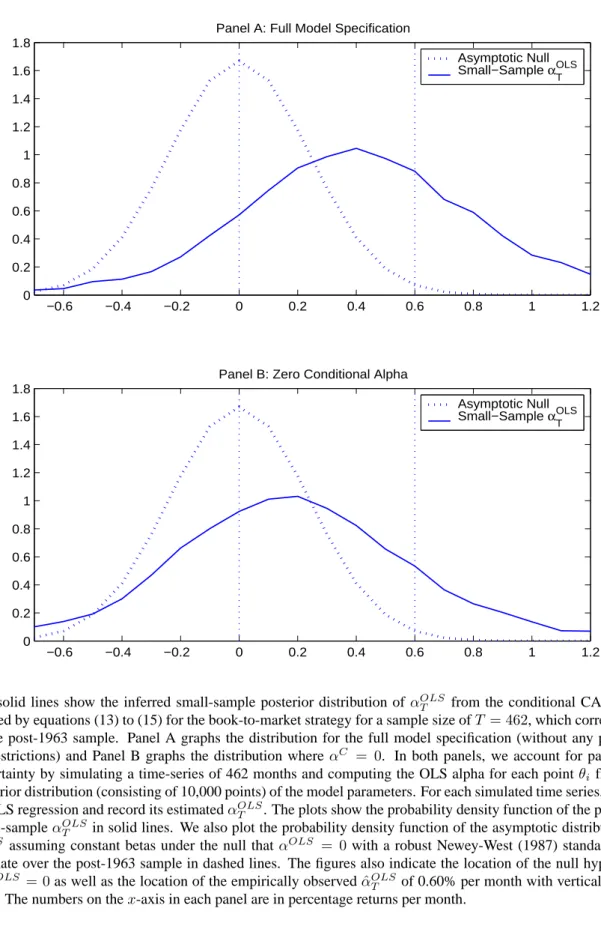
Over the post-1963 sample, a book-to-market trading strategy that goes long the highest decile portfolio of stocks sorted on book-to-market ratios (value stocks) and goes short the low-est decile portfolio of book-to-market ratio stocks (growth stocks) has an OLS alpha of 0.60% per month with a robust asymptotic p-value, ignoring time variation of betas, of less than 0.01. However, under a one-factor conditional model with time-varying betas, OLS alphas of this magnitude frequently arise in small samples of around forty years. The 0.60% per month point
estimate of the OLS alpha lies at the 67%-tile and more than 10% of the left-hand tail lies below zero. In contrast, there is little evidence that the conditional alpha is statistically signif-icant. Using a diffuse prior, more than 10% of the lower-left tail of the posterior distribution of the book-to-market strategy conditional alpha lies below zero. Only an empiricist with an extremely strong prior belief in the existence of the book-to-market premium would conclude that a book-to-market premium exists. Thus, standard OLS inference grossly overstates the statistical significance of the book-to-market premium, even when robust asymptotic t-statistics are employed because it does not take into account time-varying factor loadings.
Our research goals are related to two contemporaneous papers by Lewellen and Nagel (2005) and Petkova and Zhang (2005), who also examine whether a conditional CAPM can explain the book-to-market effect. Lewellen and Nagel (2005) contend that no reasonable de-gree of covariation in conditional betas and market risk premia can generate the high average returns associated with value stocks in the post-1963 sample. However, they do not address the non-existence of the book-to-market effect in the pre-1963 sample and do not incorporate the larger variation in betas found over the long run from 1921-2001. In addition, Lewellen and Nagel’s method of inferring the dynamics of time-varying conditional betas with a series of OLS regressions with constant betas produces inconsistent estimates of both conditional al-phas and betas. Petkova and Zhang (2005) also argue that while there is a positive correlation of shocks to the betas of value stocks and shocks to the market risk premium, this correlation is not high enough to explain the book-to-market effect. This correlation is only estimated in-directly, through instrumental proxies for conditional betas and market risk premia. Neither Lewellen and Nagel (2005) nor Petkova and Zhang (2005) examine the distortions induced by time-varying betas on the asymptotic distribution of the OLS alphas, which has as much impor-tance for statistical inference as the size of the bias in the OLS alpha.
Our results question the conventional wisdom that there exists a strong evidence of a book-to-market effect. In particular, we find that a single-factor model performs substantially better than previously believed at explaining the book-to-market premium. Whereas Davis (1994) and Davis, Fama and French (2000) argue for the existence of a book-to-market effect prior to 1963 and advocate the use of an unconditional three-factor model, they neither examine the fit of an unconditional one-factor regression nor estimate a conditional CAPM. We demonstrate that a single conditional one-factor model is sufficient to explain the average returns of book-to-market portfolios both post-1963 and over the long run. We do not claim that a conditional CAPM is the complete model for the cross-section of stock returns. In particular, more powerful
tests like the stock characteristic approaches of Daniel and Titman (1997) may be able to reject multi-factor models and their implied conditional CAPM counterparts. Nevertheless, our results show that a simple conditional single-factor model can account for a substantial portion of the book-to-market effect and that the evidence for the book-to-market effect is not as strong as previously believed.
The remainder of the paper is organized as follows. Section 2 discusses various aspects of the book-to-market portfolio returns over the long run from 1926 to 2001. In Section 3, we show that estimating time-varying betas by standard OLS estimators produces biased and inconsistent estimates with distorted asymptotic distributions. We show that the magnitude of the inconsistency and the distortion cannot be corrected without directly estimating the condi-tional betas. In Section 4, we develop a methodology for consistently estimating time-varying betas in a conditional CAPM. Section 5 presents the estimation results and examines the book-to-market effect under parameter uncertainty, time-varying factor loadings, and small sample biases. Finally, Section 6 concludes.
2
The Book-to-Market Effect Over the Long Run
We focus on the set of decile portfolios sorted on book-to-market ratios constructed by Davis (1994) and Davis, Fama and French (2000).1 We use the return on a value-weighted portfolio of all stocks listed on the NYSE, AMEX, and NASDAQ as the market return. All returns are calculated in excess of the one-month Treasury bill rate from Ibbotson Associates. Our data dif-fers from other contemporaneous studies in that we focus on the overall book-to-market effect. Loughran (1997) notes that the book-to-market effect is much stronger among smaller stocks. In contrast to our approach that focuses purely on standard book-to-market sorted portfolios, Fama and French (1993, 2005), Lewellen and Nagel (2005) and Petkova and Zhang (2005) enhance the book-to-market effect by placing greater weight on small stocks. These authors construct
2×3or5×5size and book-to-market sorted portfolios. Section 2.1 reexamines the evidence for the book-to-market effect using OLS one-factor regressions. In Section 2.2, we take a first glance at examining the time-varying nature of betas of the book-to-market portfolios.
1We obtain data on book-to-market portfolios from Kenneth French’s data library, which is at http://mba.tuck.dartmouth.edu/pages/faculty/ken.french/Data Library/.
2.1
Returns on Book-to-Market Portfolios
In Table 1, we report average monthly raw returns and volatilities together with OLS alphas and betas estimated from standard OLS regressions over various samples:
ri,t = ˆαOLST + ˆβTOLSrm,t+εOLSi,t , (1)
whereri,t is the excess stock return,rm,t is the excess market return, andεOLSi,t is an orthogonal
shock. In equation (1), we denote the estimated alpha of the OLS model as αˆOLST , with an
OLS superscript to emphasize that it is an alpha constructed under the assumptions of OLS. Similarly, we also distinguish the OLS estimate of systematic market risk exposure,βˆTOLS, with anOLS superscript. We appendαˆOLST andβˆTOLS withT subscripts to emphasize that the OLS estimates are computed over a sample size ofT. WhileαˆOLST andβˆTOLS in equation (1) should also carryisubscripts to denote that they differ across stocks, we omit them for clarity.
Panel A of Table 1 lists summary statistics for the full sample from July 1926 to December 2001, while Panels B and C cover the subsamples from July 1926 to June 1963 and from July 1963 to December 2001, respectively. For each of these subsamples, we report alphas and betas estimated by OLS, assuming constant alphas and betas over each subsample. We also report statistics on a book-to-market strategy (“BM” portfolio) which is a zero-cost portfolio that goes long the decile 10 market portfolio (value stocks) and goes short the decile 1 book-to-market portfolio (growth stocks). We compute t-statistics of the OLS alphas using Newey-West (1987) standard errors.
The first surprising result in Table 1 is that the alphas from an unconditional one-factor model are insignificant for book-to-market sorted portfolios over the long run, from 1926 to 2001. In Panel A, which uses the full 75 years of data, there is a weakly increasing relationship between the mean returns and the book-to-market ratios. However, once we control for the market beta, the individual OLS alphas become insignificant and we observe no pattern between the OLS alphas across the book-to-market deciles.2 In particular, the Newey-West t-statistic for the difference between the OLS alphas of the lowest and highest book-to-market decile portfolios is only 0.97.3 Much of the lack of a pattern in the alphas can be attributed to the weakly increasing pattern in the betas. Similarly, over the 1926-1963 subsample reported in 2Neither Davis (1994) nor Davis, Fama and French (2000) run a simple unconditional CAPM regression, or test for the significance of size or book-to-market factors relative to an unconditional one-factor model.
3A Gibbons-Ross-Shaken (1989) (GRS) test for joint significance of theα’s across all portfolios fails to reject at the 5% level over 1926-2001. Even from 1963-2001, the GRS test p-value is only borderline significant with a p-value of 0.05.
Panel B, we also fail to find any evidence of a book-to-market effect, as the difference in OLS alphas between value stocks and growth stocks is slightly negative, at -0.16% per month.
In contrast, most prior empirical work examining the book-to-market effect has focused on the period after July 1963, which we report in Panel C. In this post-1963 subsample, the uncon-ditional one-factor model fails. This latter sample has received significantly more attention than the earlier sample because data on firm book values are readily available on COMPUSTAT after this date. The raw average monthly returns of the portfolios over this period exhibit an increas-ing pattern across the book-to-market decile portfolios. The difference in returns between the value stocks and the growth stocks is 0.53% per month, with a Newey-West t-statistic of 2.16. Once we control for the market factor in an OLS regression, theαˆOLST estimates become strictly increasing and the spread in the expected returns widens to 0.60% per month, with a Newey-West t-statistic of 2.51. Unlike the pre-1963 subsample, there is no pattern in the betas across the book-to-market portfolios. This is the familiar result of Fama and French (1992, 1993), who report a strong book-to-market effect in the latter half of the century using OLS alphas.
The main difference across the two subsamples is the presence of a pattern in the OLS es-timates of betas in the pre-1963 subsample, but not in the post-1963 subsample. This finding indicates two important facts. First, betas of the book-to-market portfolios appear to vary sub-stantially across time. In the pre-1963 subsample, the OLS beta of the book-to-market strategy is positive at 0.69 and is large enough to explain the performance of the strategy. In the post-1963 subsample, the OLS beta is negative at -0.16 and can no longer explain the performance of the book-to-market strategy. The second fact is that the unconditional OLS regression of equation (1) is misspecified. The OLS specification assumes that betas are constant, but they clearly differ across the two subsamples. We now examine in greater detail the time-varying nature of betas across the long run from 1926 to 2001 and examine the implications of making inference using a misspecified OLS regression described by equation (1).
2.2
Rolling OLS Betas of Book-to-Market Portfolios
We use rolling OLS betas estimated over shorter 60-month windows to provide some evidence which suggests that the true conditional betas vary over time. While the rolling 60-month OLS regression is a common procedure for assessing time-varying betas (since as early as Fama and MacBeth, 1973), we emphasize later in Section 3 that rolling OLS betas do not directly reveal the true betas since OLS estimates of conditional betas are misspecified. Nevertheless, rolling OLS betas can provide some rough characterizations of the true conditional beta process. In
particular, the rolling OLS beta estimates provide a glimpse of what the autocorrelation and standard deviation of the true conditional betas are, and can be used to form a prior for our estimates of the true beta data-generating process.
Table 1 shows a remarkable drift in the OLS betas of the book-to-market portfolios over time. For example, in Panel B, from July 1926 to June 1963, stocks with the highest book-to-market ratios have the highest betas. The decile 10 value stock portfolio has a high average return of 1.24% per month and a corresponding highβˆTOLS of 1.66. In contrast, Panel C shows that in the post-1963 subsample, stocks with the highest book-to-market ratios have an OLS beta ofβˆOLS
T = 0.95, but a very high average return of 0.91% per month. To visually illustrate
the variation in the OLS betas that we observe in the data, we plot rolling estimates of the market OLS betas over time in Figure 1, similar to Franzoni (2004), Campbell and Vuolteenaho (2004), and Adrian and Franzoni (2005). We compute rolling estimates of the time-varying betas by regressing portfolio returns on the market return using rolling samples of 60 months.
Figure 1 shows that the rolling OLS betas of value stocks are highly persistent, but broadly reflect a downward trend. In particular, the value stock OLS betas reach a high of 2.2 during the 1940s and fall to around 0.5 in December 2001. Figure 1 also shows that the variation in the OLS betas of the growth stock portfolio is much smaller than the variation of the value stock OLS betas. Nevertheless, there is still some evidence that the OLS betas of growth stocks have a slow, mean-reverting component. However, these 60-month rolling OLS betas are, at best, 60-month averages of variation in the true conditional betas. Hence, these plots of time-varying OLS betas strongly suggest that the true conditional betas also vary over time. Since the rolling OLS betas of value stocks in Figure 1 resemble a random walk, we also expect the true conditional betas to be very persistent.
In summary, a one-factor unconditional regression can account for the book-to-market ef-fect over the full sample (1927-2001) and over the pre-1963 sample, but fails over the post-1963 sample. A one-factor unconditional regression produces large αˆOLST estimates for the book-to-market strategy only over the post-1963 sample. Moreover, betas of portfolios are not constant as assumed in standard OLS specifications, but vary significantly across time. These results have several implications. First, while the one-factor CAPM regression fails to reject the null thatαˆOLST = 0in the long run, this does not mean that we can conduct correct inference regard-ing the true conditional alpha from a data-generatregard-ing process with time-varyregard-ing betas since OLS regressions are misspecified. Similarly, while the OLS alpha of the book-to-market strategy is a largeαˆOLST =0.60% per month post-1963, this also does not necessarily imply that there exists
a positive conditional alpha in the true data-generating process. The fact that the parameters in the OLS regressions change so dramatically across samples suggests that betas, and perhaps other characteristics of the market, vary over time. Furthermore, the instability of the OLS esti-mates also suggests that the effects of small sample bias and parameter uncertainty may play a role in robust statistical inference. Since the OLS regressions are misspecified, we now develop a framework for making robust inference in a setting with time-varying risk loadings.
3
Theory
The goal of this section is to emphasize the difference between a conditional CAPM and the un-conditional one-factor regression estimated by OLS. We show that when un-conditional betas vary over time, OLS cannot provide consistent estimates of either conditional betas or conditional alphas. Section 3.1 illustrates the differences between a conditional CAPM and an uncondi-tional CAPM. In Section 3.2, we use a highly stylized model to derive closed-form asymptotic distributions for the OLS estimators (but we use a richer specification for our empirical work in Section 4). Sections 3.3 and 3.4 characterize the limiting asymptotic distributions for OLS betas and OLS alphas, respectively.
3.1
The Conditional and Unconditional CAPM
Our model is a reduced-form version of a conditional CAPM:
ri,t =αC +βtrm,t+ ¯σεi,t, (2)
whereri,t is the excess stock return,rm,t is the excess market return,εi,t is an independent and
identically distributed (IID) standard normal shock that is orthogonal to all other shocks, andσ¯ represents the stock’s idiosyncratic volatility. We define the conditional beta of stock iin the standard way as:
βt=
covt−1(ri,t, rm,t)
vart−1(rm,t)
(3) and define αC to be the conditional alpha which is the proportion of the conditional expected return that is left unexplained by the stock’s systematic exposure. We append the conditional alpha, αC, with a C superscript to distinguish it from the estimate of alpha obtained from the misspecified OLS,αOLS, from equation (1). WhileαC,βtandσ¯should also carryisubscripts
To complete the model, we specify the dynamics of the market excess return as:
rm,t =µt+ √
vtεm,t, (4)
whereµt= Et−1[rm,t]denotes the conditional mean of the market andvt=vart−1[rm,t]denotes
the conditional market volatility. Under the null of the conditional CAPM, the conditional alpha is zero,αC = 0, and the systematic risk represented byβtis solely responsible for determining
expected returns. If we reject the null hypothesis that αC = 0, we would conclude that the conditional CAPM cannot price the average excess returns of asseti.
The unconditional CAPM used by Black, Jensen and Scholes (1972), Fama and MacBeth (1973), Fama and French (1992, 1993) and others differs from the conditional CAPM in equa-tion (2) by specifying a constant beta over the entire sample period. Many authors, including Fama and French (1993), estimate the regression (1) on portfolios of stocks sorted by book-to-market ratios and reject that the OLS alpha, αˆOLST , is equal to zero. However, using the unconditional factor model in equation (1) estimated by OLS to make inference regarding the conditional CAPM in equation (2) is treacherous for several reasons.
First, Jagannathan and Wang (1996) show that if time-varying conditional betas are cor-related with time-varying market risk premia, then the conditional CAPM in equation (2) is observationally equivalent to an unconditional multifactor model:
E[ri,t] = αC +cov(βt, µt) + ¯βµ¯m, (5)
where β¯ = E(βt)and µ¯m = E(rm,t) are the unconditional means of the beta and the market
premium process, respectively. Under the null of a conditional CAPM, we would expect that the estimate of the unconditional OLS alpha, αˆOLST , captures both the conditional alpha, αC, and the interaction of time-varying factor loadings and market risk premia.
Second, Jagannathan and Wang (1996) show that we need multiple unconditional factors in the OLS regression in equation (1) to capture the same effects as the single-factor conditional model in equation (2), due to the cov(βt, µt)term in equation (5). Hence, any statement made
about the failure of an unconditional CAPM to capture the spread of average returns in the cross-section does not imply that a conditional CAPM cannot explain the cross-cross-sectional spread of average returns. Our main focus is on the ability of the conditional CAPM in equation (2) to explain the cross-section of average returns of stocks sorted by book-to-market ratios, rather than on the unconditional OLS CAPM regression in equation (1).
Third, a conditional CAPM implies an unconditional one-factor model only in the case when βt is uncorrelated withµt. In this special case, equation (5) reduces to E[ri,t] = αC +
¯
βµ¯m. However, when conditional betas and market risk premia are correlated, OLS fails to
provide consistent estimates of both the conditional alpha and the conditional betas in equation (2). Moreover, the degree of the inconsistency depends on unknown parameters driving the conditional beta process that are not directly observed. Hence, any inference on the conditional CAPM in equation (2) cannot be made on the basis of OLS estimates of the unconditional one-factor model in equation (1). Finally, the limiting distributions of the OLS alphas and betas (αˆOLST andβˆTOLS in equation (1)) are significantly distorted from their conventional OLS asymptotic distributions that assume constant factor loadings. We now illustrate each of these points in the context of a very simple model for which we can analytically derive the limiting distributions ofαˆOLST andβˆTOLS.
3.2
A Simple Model
We first consider the simplest possible setting where stock i’s excess return, ri,t, is driven by
a time-varying beta process. Suppose that in the true conditional model (2), βt and rm,t are
stochastic and correlated with an unconditional correlation of ρmβ. In this simplest possible
setting, we specify that:
βt IID∼ N( ¯β,σ¯β2)
and rm,t IID∼ N(¯µm,σ¯2m), (6)
where β¯is the unconditional beta, σ¯β2 is the unconditional variance of beta,µ¯m is the
uncon-ditional mean of the excess market return, σ¯m2 is the variance of the excess market return, and corr(rm,t, βt) = ρmβ. In the statistics literature, this is a standard random coefficient model (see,
for example, Cooley and Prescott, 1976).
Our goal is to characterize the asymptotic distribution of the OLS estimators:
ˆ αOLST = 1 T T X t=1 ri,t−βˆTOLS 1 T T X t=1 rm,t and βˆTOLS = Ã 1 T T X t=1 (rm,t−r¯m)2 !−1Ã 1 T T X t=1 (rm,t −r¯m)ri,t ! , (7) where r¯m = (1/T) P
rm,t represents the sample average of the excess market return, under
the data generating process of equation (6). We relegate the full derivation of the asymptotic distribution of√T(ˆαOLST −E[ˆαOLST ])and√T( ˆβTOLS −E[ ˆβTOLS])to Appendix A.4
We note that the OLS alpha and beta estimates in equation (7) are not pivotal statistics, as their distribution depends explicitly on the parameters of the data-generating process in equation (6). But, the OLS alpha is precisely the statistic most often used by researchers to judge the significance of any CAPM anomaly. Our focus is not to develop a pivotal statistic to estimate time-varying betas, but rather to show how the OLS alpha and beta distributions are affected by time-varying betas. Thus, we point out that inference based on OLS alpha and beta estimates are unreliable in the presence of time-varying factor loadings.
3.3
Asymptotic Distribution of
√
T
( ˆ
β
TOLS−
E[ ˆ
β
TOLS])
To understand the distortions that OLS induces on a system with time-varying betas relative to the standard case, it is helpful to write the residual term,εOLSi,t , of the regression (1) in the form of an omitted variable(βt−β¯)rm,t:
εOLSi,t = (βt−β¯)rm,t+ ¯σεi,t. (8)
Unlike the usual case of a constant beta, this omitted variable is a product of two normal distri-butions and can cause at least three distinct problems in the OLS estimates. First, the residuals are heteroskedastic. Second, in practice, βt is likely to be very persistent (but is assumed to
be IID in this simple setting for tractability), which leads to serial correlations in the residuals. Both the problem of heteroskedasticity and serial correlation inεOLSi,t can, in principle, be cor-rected by a heteroskedasticity and autocorrelation consistent (HAC) estimator like Newey and West (1987). Note that this is only an asymptotic correction, so a HAC estimator still ignores the effect of any small sample distortion and bias. The major problem that cannot be corrected by using a HAC estimator is that the OLS residuals, εOLSi,t , are correlated with the regressor,
rm,t, which leads to biased and inconsistent OLS estimates: E[ ˆβOLS T ] = ¯β+ ρmβσ¯β ¯ σm ¯ µm. (9)
inconsistent (see, for example, Greene, 2002), but they do not derive the limiting distribution of the OLS estimators. As we show, this derivation is non-trivial as it involves quadratic functions of normals, but this exercise is necessary to interpret both the bias and the sampling dispersion of the OLS estimates. Foster and Nelson (1996) develop a series of rolling weighted OLS regressions, where the optimal weights are a function of the underlying data generating process, that can provide efficient estimates of conditional betas. This case is different to the standard OLS regressions run over the whole sample that are common in the literature. Foster and Nelson also do not consider asymptotic distributions of OLS alphas with time-varying conditional betas.
The magnitude of the inconsistency ofβˆTOLS in equation (9) depends on the unknown pa-rameters β¯, ρmβ, σ¯β, and µ¯m. Lewellen and Nagel (2005) make inferences on the properties
the conditional alphas and the conditional betas by estimating a series of high frequency OLS regressions in subsamples. However, note that the inconsistency term in equation (9) depends on the ratio ofσ¯βtoσ¯mwhich is invariant to the sampling frequency and can be potentially very
large. Moreover, even if subsample regressions are used to estimate OLS betas, this does not remove the inconsistency since the conditional betas continue to vary within windows. Hence, there is no way to correct for the inconsistency without knowingβ¯,ρmβ, andσ¯β, and these
pa-rameters can only be obtained by directly estimating the conditional beta series. In data, since the market risk premia and the variance of the market change over time (see Schwert, 1989), the magnitude of the inconsistency of the OLS estimate,βˆTOLS, is also time-varying. The OLS beta provides a consistent estimate of the mean of the true beta process only in the case when the betas are uncorrelated with the market return,ρmβ = 0.
There is also a distortion of the standard limiting distribution induced by the presence of time-varying betas. The asymptotic distribution of√T( ˆβTOLS −E[ ˆβTOLS])is given by:
√ T( ˆβOLS T −E[ ˆβTOLS]) d →N µ 0,(3 + 12ρ2 mβ)¯σβ2 + (1−ρ2mβ)¯µ2m ¯ σ2 β ¯ σ2 m + σ¯2 ¯ σ2 m ¶ . (10) The last term for the asymptotic variance is σ¯2/σ¯m2, which is the asymptotic variance for the standard OLS case without any time variation in the betas (σ¯β = 0). The other two terms reflect
the contribution of the endogenous regressorβtthat increases the variance of theβˆTOLS estimator
relative to the constant beta case.
This increase is not small, even if the betas are uncorrelated with the market return. For example, suppose that ρmβ = 0, µ¯m = 0.0066, and σ¯m = 0.055, where the excess market
parameters are calibrated from the sample mean and sample standard deviation of the monthly excess market returns over 1927-2001. We set the stock idiosyncratic volatility at σ¯ = 0.06 and set the σ¯β parameter of the book-to-market portfolios to be 0.468. The last parameter
represents the monthly unconditional standard deviation of the betas, which we discuss below in Section 5.1. Then, the ratio of the true asymptotic variance in equation (10) to the standard OLS asymptotic variance is approximately two. This is a conservative estimate because ρmβ
is unlikely to be zero. Hence, the true limiting variance ofβˆTOLS is likely to be larger than the variance implied by standard OLS theory. Therefore, even if we know the correct adjustment for the inconsistency of theβˆTOLS estimator, we cannot at all be confident about the precision of the estimate of the conditional beta.
3.4
Asymptotic Distribution of
√
T
(ˆ
α
OLST−
E[ˆ
α
TOLS])
Jaganathan and Wang (1996) and Lewellen and Nagel (2005), among others, note that the OLS estimate of alpha, αˆTOLS, is a biased estimate of the conditional alpha, αC, in the conditional CAPM specified in equation (2). In our simple model,E[ˆαOLST ]is given by:
E[ˆαOLST ] = αC +ρmβσ¯β ¯
σm
(¯σm2 −µ¯2m). (11) Note thatαˆTOLS provides a consistent estimate of αC only when the market return process and the conditional betas are uncorrelated. If ρmβ 6= 0, then direct knowledge of the conditional
beta process is required to correct for the inconsistency of αˆOLS. As a rough estimate, if we assume thatρmβ = 0.1(see below),σ¯β = 0.468,µ¯m = 0.0066, andσ¯m = 0.055, then equation
(11) indicates thatαˆTOLS overstates the true value ofαC by over 0.26% per month.5
In our simple model, the asymptotic distribution of the OLS estimate,αˆOLST , is given by:
√
T(ˆαOLST −E[ˆαOLST ]) d →N µ 0,10ρ2mβµ¯2mσ¯β2 + (1−ρ2mβ)(¯σm4 + ¯µ4m)σ¯ 2 β ¯ σ2 m + (¯σm2 + ¯µ2m)σ¯ 2 ¯ σ2 m ¶ . (12) The asymptotic variance of αˆOLST in equation (12) has three terms. The third term, (¯σm2 +
¯
µ2
m)¯σ2/σ¯m2, is the regular asymptotic variance for the OLS estimate for the intercept term in
an environment with non-stochastic betas. In cases where σ¯β is large, the asymptotic variance
of αˆOLST increases substantially whenσ¯β is not zero, relative to the standard OLS asymptotic
variance. Again, we cannot compute the degree of distortion relative to the regular OLS stan-dard error case without knowingσ¯β andρmβ. Moreover, these parameters cannot be estimated
without knowing the conditional, latent beta series. Using asymptotic theory, we can estimate the increase in the asymptotic variance ofαˆOLST induced by the time-varying regressors by using a HAC estimate of the variance only in the special case whenρβm = 0. Whenρβm 6= 0, HAC
estimators are invalid.
In summary, we cannot obtain consistent estimates of conditional betas or alphas by OLS. Neither the adjustments for the magnitude of the inconsistency nor the corrections for the dis-tortions in the asymptotic variances of the OLS estimators can be accomplished without direct 5The term we analyze here is not fully present in the empirical analysis of conditional alphas of Lewellen and Nagel (2005) because they (counter-factually) assume that OLS is consistent within each subsample. Our method consistently accounts for the time variation in conditional betas within a given window where Lewellen and Nagel have assumed the OLS betas are consistent.
knowledge of the dynamics of the conditional beta process. We now propose a richer model with time-varying conditional betas, time-varying market risk premia, and time-varying systematic volatility and explain how such a model can be estimated.
4
A Conditional CAPM with Time-Varying Betas
The asymptotic distributions of√T( ˆβTOLS −E[ ˆβOLS])and√T(ˆαOLST −E[ˆαOLS])in equations (10) and (12) are likely to understate the true variation of βˆTOLS and αˆOLST in small samples for two reasons. First, we expect that rather than the conditional betas being drawn from an IID process, conditional betas are more likely to incorporate predictable, slow, mean-reverting components. While we derived the asymptotic distributions using a Central Limit Theorem that can be generalized to incorporate persistence inβt, a high autocorrelation of theβtprocess will
cause the asymptotic variance to significantly understate the true variance in small samples. Second, the market process is also empirically not a normal IID process. A more realistic em-pirical description of the market return is that it also incorporates persistent components both in its conditional mean and conditional volatility. The addition of time-varying components in the market return process further distorts the asymptotic inference of the OLS estimators. For our empirical application, we enrich the simple model of the previous section to incorporate persis-tent conditional betas, time-varying market risk premia, and stochastic systematic volatility.
4.1
The Model
In our fully specified conditional CAPM, we assume that the latent conditional betas in equation (2) follow an AR(1) process:
ri,t = αC +βtrm,t+ ¯σεi,t
and βt = β0+φββt−1+σβεβ,t, (13)
whereβtrefers to the conditional beta of stockidefined in equation (3). Again, in equation (13),
αC, β
t,σ¯,β0, φβ, andσβ should all haveisubscripts, but we omit them for simplicity. We are
interested inri,trepresenting the returns on the book-to-market strategy. Following the standard
set-up of a conditional factor model where the idiosyncratic volatility shocks are uncorrelated with systematic components, we specifyεi,tto be drawn from an IID normal distribution that is
We expect that the conditional betas in equation (13) vary slowly over time withφβclose to
one. This view is suggested both from economic theory and from prior empirical studies. For example, Gomes, Kogan and Zhang (2003), suggest that betas are a function of productivity shocks, which are often calibrated with an autocorrelation of 0.95 at the quarterly horizon. This translates into a monthly autocorrelation of conditional betas above 0.98. In Santos and Veronesi (2004), stock betas change as the ratio of labor income to total consumption changes, which is also a highly persistent variable. Since the firms in the book-to-market portfolios change over time, portfolio reconstitution could also cause time variation in the portfolio betas. Since the OLS rolling betas in Figure 1 have a wide range, we expect that the conditional shocks to the true betas of the book-to-market portfolios can be quite variable, orσβ could be large. In
data, Fama and French (1997) also report substantial variation in factor loadings for industry portfolios, while Ferson and Harvey (1999) show that there is a large variation in the market betas of portfolios sorted by size and book-to-market ratios. Hence, our prior is that βt should
be highly persistent and conditional shocks toβtcan potentially be large.
We further specify that the excess market return, rm,t, in equation (4) has a conditional
market risk premium,µt, and exhibits stochastic systematic volatility,vt:
rm,t =µt+ √ vtεm,t, (14) where µt = µ0+φµµt−1+σµεµ,t and lnvt = v0+φvlnvt−1+σvεv,t. (15)
The shocks,εm,t,εµ,tandεv,t, are normally distributed zero mean, unit standard deviation,
nor-mally distributed shocks that are potentially correlated. In equation (15), we allow the market risk premium to be a slowly mean-reverting latent process. This is the same specification used in the portfolio allocation literature, beginning with Merton (1971). We model log volatility as a latent AR(1) process, following Jacquier, Polson and Rossi (1994). The log process restricts volatility to be positive and induces fat tails in the distribution for the market return. Since Brandt and Kang (2004) find that the correlation between εm,t andεµ,tis insignificant, we set
this correlation to be zero. We also specifyεm,t andεv,t to be orthogonal. However, we letεµ,t
andεv,thave a correlation ofρµv. This captures a leverage effect, and allows market conditional
expected returns and stochastic volatility to move together. To allow the market risk premia to be correlated with conditional betas, we letεµ,tandεβ,tin equations (13) to (15) have a non-zero
The OLS alpha,αˆTOLS, estimated from the regression (1) is an implied function of the pa-rameters θ = (µ0 φµ σµ v0 φv σv ρµv β0 φβ σβ σ α¯ C ρµβ) of the model and the sample
size T. Similar to the setting of our simple model in Section 3.2, the limiting distribution of
αOLS
T depends on the beta process and the market return process. However, the asymptotic
dis-tribution of the OLS alpha in our richer empirical specification (equations (13) to (15)) cannot easily be derived in closed form. In our estimation method, we directly estimate the conditional betas, {βt}, and the conditional alpha, αC, and we construct the implied distribution of αˆOLST
numerically. We stress that our implied distributions of the OLS estimatesαˆOLST andβˆTOLS are based on the null of the model in equations (13) to (15). However, we show that the model matches the evidence in data on rolling OLS betas and expect that inference under alternative models which allow similar time variation in betas and the market risk premium to also induce large distortions in the distributions of the OLS statistics relative to their standard distributions. The reduced-form conditional CAPM in equations (13) to (15) falls within the class of conditional CAPM models developed by Harvey (1989), Shanken (1990), Ferson and Harvey (1991, 1993, 1999), Cochrane (1996), and Jagannathan and Wang (1996). Most of these stud-ies use instrumental variables to model the time variation of betas as a linear function of the instruments. Our betas are also time-varying, but instead of relying on instrumental variables, we parameterize the beta itself as an endogenous latent process. This has the advantage of not relying on exogenous predictor variables to capture time-varying betas and avoids any poten-tial omitted variable bias from mis-specifying the set of predictor variables (see Harvey, 2001; Brandt and Kang, 2004). Instead, we infer the betas directly from portfolio returns. Second, we directly model the variation in the betas across time. Campbell and Vuolteenaho (2004), Adrian and Franzoni (2004), Franzoni (2004), and Lewellen and Nagel (2005) document that the betas of book-to-market portfolios change over time, but they do so by estimating constant beta models over different subsamples of data. Section 3.3 shows that this procedure leads to biased and inconsistent estimates with distorted asymptotic distributions.
A special case of our model is an unconditional CAPM, which arises whenρµβ = 0. The
model explicitly captures the time variation in market risk premia that previous empirical studies show is important, and whenρµβ 6= 0, the unconditional CAPM does not hold but a conditional
CAPM applies. Rather than using GARCH processes to model conditional betas (see, for ex-ample, Bekaert and Wu, 2000), our model uses a log volatility model. In GARCH models, betas are time-varying but the variations in the betas are strictly driven by past innovations in returns and do not have independent random components. Danielsson (1994), among others, finds that
the GARCH family of models does not remove all non-linear dependencies in stock return data, while autoregressive stochastic volatility models provide better goodness-of-fit for stock return dynamics.
While the model generates heteroskedasticity, one feature of the data that the model is not designed to capture is time-varying idiosyncratic volatility. In the return equation (13), we assume that idiosyncratic volatility is constant at σ¯. Campbell et al. (2001) show that the id-iosyncratic volatility has noticeably trended higher for individual stocks over the 1990s. In-corporating time-varying idiosyncratic volatility would introduce a difficult identification prob-lem between time-varying betas and idiosyncratic risk. We apply the model to stock portfolios, where idiosyncratic risk is lower than at the firm level. Nevertheless, incorporating time-varying idiosyncratic risk would only exacerbate the large variances in OLS alphas that we document, and hence, by ignoring time-varying idiosyncratic risk, our analysis is conservative.
4.2
Estimation
We estimate the model over the full sample, from 1926-2001, to use all available data to pin down the dynamics of the beta process. After estimating the data on the full sample, we ex-amine the small sample distribution of OLS alphas or conditional alphas. In particular, we are especially interested in small samples of the same length as the post-1963 sample, which is the sample where the OLS alpha appears to be significant using conventional t-statistics. Estimating the model only over the short post-1963 sample to infer the distribution of OLS or conditional alphas over the post-1963 period is inefficient and ignores valuable information about the time variation of betas over the long run.
We use a Markov Chain Monte Carlo (MCMC) and Gibbs sampling estimation method that consistently estimates conditional alphas and betas, incorporates the effect of parameter uncer-tainty, and measures the effect of small sample bias. Appendix B provides a full description of the estimation method.6 There are three main reasons we use a Bayesian estimation strategy.
First, conditional on the time series of conditional betas ({βt}), time-varying market risk
premia ({µt}), and time-varying systematic volatility ({vt}), the stock return,ri,t, in equation
(13) is normally distributed. However, the likelihood function for ri,t and rm,t is difficult to
6Other similar models are esimated by Liu and Hanssens (1981), Lamoureux and Zhou (1996), Johannes, Polson and Stroud (2002), Johannes and Polson (2003), Jones (2003), Han (2004), and Jostova and Philipov (2005) with Bayesian methods; Harvey, Solnik and Zhou (2002) with GMM; and Brandt and Kang (2004) with simulated maximum likelihood.
derive in closed form because the latent variables{βt},{µt}, and{vt}must be integrated out.
This makes maximum likelihood estimation methods difficult to use. Other classical estima-tion methods, like Generalized Method of Moments (GMM), also entail a potentially difficult optimization problem. In contrast, the Gibbs sampler is fast because it involves drawing from well-defined conditional distributions.
Second, while the asymptotic distribution of the OLS alphas can be derived in closed-form for our simple IID model in Section 3, the asymptotic distribution of the OLS estimators in the conditional CAPM is difficult to derive. MCMC provides posterior distributions whose means can be interpreted as parameter estimates and the inferred estimates of the time series of betas, market risk premia, and systematic volatility are generated as a by-product of the estimation. The estimation method also allows us to extract the exact finite sample distributions of OLS alphas from the posterior distributions of the parameters. We compute the posterior distributions for the OLS alpha,αˆOLS
T , for the limiting case whereT =∞, and over a finite sample whereT
corresponds to the post-1963 sample period. Then, we compare these estimates of asymptotic distribution of αˆOLST and small sample distribution of αˆOLST directly to the estimates of the conditional alpha,αC.
Finally, we can impose some prior information on some of the parameters, like the param-eters that determine the speed of mean reversion of µt and βt that would otherwise lead to
identification problems (see the discussions in Brennan, 1998; Johannes, Polson and Stroud, 2002). In particular, the mean-reversion parameter of the betas (φβ) is difficult to pin down.
With non-informative priors, the estimate ofφβ is almost zero, and the estimates for the betas
become degenerate, making βt ≈ ri,t/rm,t. This makes the likelihood function infinite. We
have strong prior beliefs from economic theory that the betas are persistent, so φβ should be
close to one, but they must also be bounded above by one to maintain stationarity. Lamoureux and Zhou (1996), Johannes, Polson and Stroud (2002), and Johannes and Polson (2003) all im-pose informative priors over mean-reversion parameters in related models. We now discuss our choice of prior forαC, but detail the full specification of all the other priors in Appendix B.
4.3
Priors on
α
CInference regarding the conditional alpha, αC, is of critical importance to measuring the eco-nomic and statistical significance of the book-to-market premium. We specify informative pri-ors over αC that range from no prior belief about the value of αC to a dogmatic belief that an
αC must exist. Prior beliefs aboutαC are represented by the distribution: αC ∼N¡µpαC,(σ p αC)2 ¢ , (16)
whereµpαC is the prior mean and(σ
p
αC)2is the prior variance. Ifµ
p
αC = 0andσ
p
αC is very small, then the researcher believes dogmatically in the conditional CAPM, while a positiveµpαC and a very small σpαC represents a researcher with a strong prior that the book-to-market premium is positive. In contrast, setting σαpC = ∞ or allowing σ
p
αC to be sufficient large, represents an effectively diffuse prior that assumes no a priori knowledge about the strength of the value premium.
An alternative specification of priors for the conditional alpha is given by Pastor and Stam-baugh (1999) and Pastor (2000), who specify the prior to be directly proportional to idiosyn-cratic volatility:
αC|σ¯ ∼N(µp
α, ησ¯2), (17)
whereηis the prior degree of belief in the conditional CAPM. Whenη=∞, mispricing relative to the conditional CAPM is completely unrestricted, whileη= 0corresponds to dogmatic faith in the conditional CAPM. In the Pastor-Stambaugh prior in equation (17), the prior on αC is directly linked to the idiosyncratic volatility, which reduces the probability of drawing high Sharpe ratios. Hence, using the Pastor-Stambaugh prior would make us less likely to reject the null of a conditional CAPM. In contrast, our choice of prior on αC in equation (16) specifies no mechanical link betweenαC andσ¯. With our prior in equation (16), draws of high posterior Sharpe ratios are more likely than under the Pastor-Stambaugh prior and, thus, we bias our results in favor of finding evidence against the conditional CAPM.
4.4
Priors on Time-Varying Betas
Using Figure 1, we can extract some prior information about the latent conditional beta process. Just as the OLS betas are very persistent, we also expect the conditional betas to have slow moving persistent components. We treat the standard deviation of the rolling OLS betas as a sample statistic and compute a similar statistic from our conditional beta estimates to judge the goodness-of-fit of the model. What rolling OLS betas cannot provide, however, are estimates of the true variability of conditional betas, the correlation of conditional betas with market risk premia, or precise estimates of the conditional beta at a particular point in time. Only direct estimates of the conditional betas can accomplish this.
In Table 2, we examine the autocorrelations and standard deviations of the rolling OLS be-tas of the highest (lowest) book-to-market decile portfolio, which are the value (growth) stocks, along with the book-to-market strategy. We report the 60th order autocorrelation since it is the lowest order autocorrelation that does not use overlapping information. We then compute the first-order autocorrelation implied by an AR(1) process. The implied monthly autocorre-lations are highly persistent, with an estimate of 0.993 for the book-to-market strategy. This is a conservative estimate as estimates of autocorrelations are biased downwards in small sam-ples. We compute a tight standard error of 0.003 for the first-order autocorrelation using the delta-method. Although the OLS betas are inconsistent estimates of the conditional betas, we assume that the true conditional betas have a persistence of the same order of magnitude as the persistence of the non-overlapping autocorrelations implied by the rolling OLS betas.
Table 2 also reports the unconditional standard deviations of the rolling 60-month OLS betas. For the growth stock and the value stock portfolios, they are 0.11 and 0.38, respectively. For the book-to-market strategy, the rolling OLS betas exhibit a large degree of time variation, with a volatility of 0.47. Below, we show that rolling averages implied by our estimates of conditional betas closely match this statistic. Armed with this knowledge about the rolling averages of OLS betas, we now directly infer the true conditional betas,{βt}, by estimating the conditional CAPM in equations (13) to (15).
In our estimation, we are especially careful not to increase the variance of the conditional betas in a manner that implies implausibly large stock return volatility. A model that implies a large stock return variance can potentially produce very disperse posterior distributions with little information. We impose the constraint on our parameter estimates that the total variance of stock returns is kept constant at the level observed in the data. Thus, by construction, systematic and idiosyncratic volatility sum to the observed total volatility of stock returns in data.
5
Empirical Results
We present our estimates of the conditional CAPM with time-varying betas in Section 5.1. Section 5.2 characterizes the posterior distribution of the conditional alphas of the book-to-market strategy and Section 5.3 reports the unconditional OLS alphas implied by our model. In Section 5.4, we consider the additional effects induced by finite sample bias.
5.1
Parameter Estimates of the Conditional CAPM
Table 3 reports the parameter estimates for the conditional CAPM described by equations (13) to (15). We estimate these models using the value stock portfolio, the growth stock portfolio, and the book-to-market strategy. To compute the estimates in Table 3, we use an effectively diffuse prior withµpαC = 0and σ
p
αC = 1.00% per month in the prior forαC in equation (16). ChangingµpαC = 1.00%or using values ofσ
p
αC larger than 1.00% per month produces virtually identical results. Table 3 reports the mean and standard deviation of the posterior distribution of each parameter. We first characterize the market return process and then investigate the effects of time-varying conditional betas.
The Market Factor
Table 3 shows that the estimated market risk premium process is persistent, with a monthly autocorrelation ofφµ = 0.956. Shocks to the conditional mean are not small, with a volatility
ofσµ = 0.40%per month. These estimates translate to an unconditional volatility of monthly
market risk premium of 1.36% and unconditional volatility of annual market risk premium of approximately 2.0% per annum. The log variance, lnvt, is also a persistent process with
an autocorrelation of φv = 0.941 and is slightly conditionally negatively correlated with the
conditional mean of the market (ρµv =−0.093). This is consistent with many studies that find
a leverage effect with negative correlations between market volatility and expected returns (see, for example, Campbell and Hentschel, 1992).
In Figure 2, Panel A, we plot estimates of the implied market risk premia and conditional systematic volatility. The estimates of the market risk premia are fairly smooth, but they have moderately large standard error bounds. Pinning down the market risk premia is notoriously difficult. Johannes and Polson (2003) report that for their estimates of NASDAQ expected returns, even a one standard deviation bound often includes zero. Nevertheless, Panel A of Figure 2 shows that market risk premia increase during the late 1930s and the early 1950s, and decline during the 1960s. More recently, market expected returns increase steeply around the time of the OPEC oil shocks in the 1970s. Over the late 1980s and early 1990s, market expected returns are fairly stable but decrease dramatically during the bull market of the late 1990s. During the year 2000, market expected returns start to increase, coinciding with the onset of the last recession. In most of these episodes, volatility moves in opposite directions to expected returns, as shown in Panel B. Our estimate of market volatility reaches a high of close to 17% per month in the early 1930s, and also increases during World War II, the mid-1970s,
the 1987 crash, and around the end of the century from 1998-2001.
Time-Varying Beta Estimates
From the estimates of the latent beta process in Table 3, the implied unconditional beta of the value (growth) stock portfolio is 1.21 (1.01). For the book-to-market strategy, the implied unconditional beta is 0.11. Hence over the whole sample, value stocks do have slightly higher betas than growth stocks, but the difference is small. Table 3 also reports that the latent betas, while highly persistent, are fairly volatile. The conditional volatility of the latent betas for value stocks is fairly large at 0.168 per month, compared to 0.132 per month for growth stocks. In comparison, the conditional volatility of the betas for the book-to-market strategy is a modest 0.065 per month.
For the book-to-market portfolios, the correlation between shocks to the conditional betas and shocks to the market risk premium, ρµβ, is large and positive. For value (growth) stocks,
ρµβ is 0.759 (0.882). For the book-to-market strategy, the posterior mean ofρµβ is 0.408 with
a posterior standard deviation of 0.127. Since the unconditional volatility of the market risk premium is 1.36% per month and total market volatility is fixed at 5.5% per month, this implies an unconditional correlation between betas and market returns of 0.1. The large value of ρµβ
has several implications. First, from equation (5), an unconditional one-factor CAPM cannot be the correct specification for risk sinceρµβ 6= 0. Second, equations (9) and (11) show that the
OLS estimates of betas and alphas are biased and inconsistent. Third, equation (12) shows that the distribution ofαˆOLST is distorted from its regular OLS asymptotic distribution. We examine theαC estimates and the implied OLS alpha distributions in detail below.
In Figures 3 and 4, we plot the posterior mean of the time-varying betas produced by the Gibbs sampler. Figure 3 shows the estimates for the value and growth portfolios. The estimated betas of the value stock portfolio exhibit greater variation than the betas of the growth stock portfolio. The conditional betas of value stocks wander from over 3.0 during the late 1930s to below 0.5 in 2001. In contrast, the conditional betas of growth stocks remain in a fairly close neighborhood around 1.0. Figure 4 graphs the estimates for the book-to-market strategy. The conditional betas of the book-to-market strategy reach a high of above 1.5 near-1940, and decline to close to negative 0.5 at the end of 2001. Figure 4 also shows the one posterior standard deviation bound, which is around 0.5 across the whole sample.
We can compare the conditional variability of the estimated latent betas to the standard deviation of rolling 60-month OLS betas as a specification test of our model estimates. To
confirm that the estimates of conditional volatility of the time-varying betas implied by the model match the variability of rolling OLS betas found in the data, we compare the variability of 60-month moving averages of the inferred betas of the book-to-market strategy in Figure 4 to the variability of the 60-month rolling OLS betas reported in Table 2. The match is almost exact. For the book-to-market strategy, the implied rolling 60-month beta average volatility is 0.46, compared with 0.47 in data. Hence, our conditional beta estimates implies rolling betas with a similar degree of variability as the rolling OLS betas from the data.
The large swings of our conditional betas are also consistent with the widely differing point estimates of the OLS alphas across subsamples in Table 1. Taking the posterior mean of the time series of the conditional betas,{βˆt}, we compute the differencerit−βˆtrmtacross subsamples.
In the pre-1963 sample, the mean conditional beta is 0.47, the book-to-market strategy returns 0.43% per month, while the excess market return yields 0.85% per month. Thus, in the pre-1963 sample, the mean value ofrit−βˆtrmtis 0.03% per month, consistent with an OLS alpha
of close to zero. In contrast, over the post-1963 sample, the average conditional beta is -0.11, the book-to-market strategy yields 0.53% per month, and the average market excess return is 0.47% per month. Thus, the mean value of rit −βˆtrmt over the post-1963 sample is 0.58%
per month, which is very close to the empirically observed OLS alpha of 0.60% per month reported in Table 1. This suggests that although our model has a constantρµβand constantαC,
the model is capable of generating large differences in OLS alphas in specific sample periods. In particular, the time series of the posterior mean of the conditional betas is consistent with the low (high) OLS alpha in the pre-1963 (post-1963) sample period for the book-to-market strategy.
5.2
Conditional Alphas of the Book-to-Market Strategy
Inference regarding the conditional alpha, αC, is crucial for judging the fit of the conditional CAPM to explain the value premium. In Table 4, we report the posterior distribution of αC of the book-to-market strategy. To incorporate various prior views that investors may hold on the strength of the book-to-market effect, we specify several prior distributions, rather than using just one diffuse prior. The priors forαCin equation (16) range from an effectively uninformative prior withµpαC = 0andσpαC = 1.00%per month to a highly informative prior withµpαC = 0.60% per month andσαpC = 0.10%per month. Since a mean of 0.60% per month corresponds to the
ˆ
αOLS
T estimate of the book-to-market strategy over the post-1963 sample (see Table 1), priors
prior, we report the percentile breakpoints, the mean and the standard deviation of the posterior distribution ofαC.7
When we use a prior onαC with a mean of zero, the value of 0.00% per month lies well above the 10%-tile breakpoint of the posterior, regardless of the standard deviation of the prior. In particular, for the effectively diffuse prior with µpαC = 0and σ
p
αC = 1.00%per month, the value corresponding to the 10%-tile is -0.01% per month. Hence, an uninformed agent would conclude that the conditional alpha of the book-to-market strategy is insignificantly different from zero. To argue in favor of a strong book-to-market effect, an agent would need to have a strong prior on αC that has a mean of 0.60% per month and a standard deviation of 0.30%
per month or tighter. Under this prior, the posterior distribution ofαC has a lower left-hand tail probability of less than 2.5% for observing a conditional alpha less than zero.
In summary, Table 4 shows that once we account for the time-variation in betas and mar-ket risk premia, the evidence against a conditional CAPM is weak using the book-to-marmar-ket portfolios. In contrast, only the misspecified OLS inference that assumes constant betas based strictly on the post-1963 sample would suggest strong evidence of a book-to-market effect: the OLS alpha has a p-value of 0.006, corresponding to a Newey-West t-statistic of 2.51. However, after accounting for time-varying, conditional betas, only an empiricist with a very strong prior belief in a book-to-market premium would conclude that a conditional CAPM cannot account for the average returns of stocks sorted by book-to-market ratios over the long run.
5.3
OLS Alphas of the Book-to-Market Strategy
We showed in Section 3 that in the simplest IID environment with correlated time-varying betas and market risk premia, the OLS estimate of alpha, αˆOLST , is inconsistent and the asymptotic distribution of√T(ˆαOLST −E[ˆαTOLS])is significantly distorted from its standard OLS distribu-tion with constant betas. We now show that the distordistribu-tion between αC and αˆOLST are further magnified when we allow for persistent, time-varying betas.
We compute the implied distribution of the OLS alpha, αTOLS (denoted without a hat to signify it is a random variable), for a sample size ofT from the Gibbs sampler. We first compute the limiting distribution of the OLS alpha as T → ∞, which we denote as αOLS. For each observation in the posterior distribution of the model parameters θ, we compute the value of
αOLS
T that would result if the data are generated according to equations (13) to (15). We compute
7The posterior distributions ofαC are largely unaffected by the estimation of the market process, even if we