Are macroeconomic density forecasts informative?

Are macroeconomic density forecasts 

informative? 

Article 

Accepted Version 

Creative Commons: Attribution­Noncommercial­No Derivative Works 4.0 

Clements, M. (2018) Are macroeconomic density forecasts 

informative? International Journal of Forecasting, 34 (2). pp. 

181­198. ISSN 0169­2070 doi: 

https://doi.org/10.1016/j.ijforecast.2017.10.004 Available at 

http://centaur.reading.ac.uk/72924/ 

It is advisable to refer to the publisher’s version if you intend to cite from the 

work.  See 

Guidance on citing  

.

To link to this article DOI: http://dx.doi.org/10.1016/j.ijforecast.2017.10.004 

Publisher: Elsevier 

All outputs in CentAUR are protected by Intellectual Property Rights law, 

including copyright law. Copyright and IPR is retained by the creators or other 

copyright holders. Terms and conditions for use of this material are defined in 

the 

End User Agreement  

. 

www.reading.ac.uk/centaur  

CentAUR 

Are Macroeconomic Density Forecasts Informative?

Michael P. Clements

ICMA Centre,

Henley Business School,

University of Reading,

Reading RG6 6BA

October 3, 2017

Abstract

We consider whether survey density forecasts (such as the in‡ation and output growth histograms of the US Survey of Professional Forecasters) are superior to unconditional density forecasts. The uncon-ditional forecasts assume that the average level of uncertainty experienced in the past will prevail in the future, whereas the SPF projections ought to be adapted to current conditions and the outlook at each forecast origin. The SPF forecasts might be expected to outperform the unconditional densities at the shortest horizons, but this does not transpire to be the case for the aggregate forecasts of either variable, or for the majority of the individual respondents for forecasting in‡ation.

Keywords: probability distribution forecasts, aggregation, Kullback-Leibler information criterion. JEL classi…cation: C53.

I am grateful to two anonymous referees, an Associate Editor, and Editor Dick van Dijk for helpful comments, as well as to conference participants at the International Symposium on Forecasting, Santander, 2106

1

Introduction

There has been much interest in survey forecasts in recent years, driven in part by the opportunities they o¤er to test theories of expectations-generation (see, e.g., Pesaran and Weale (2006), Coibion and Gorodnichenko (2012, 2015) and Andrade and Le Bihan (2013), amongst many others) and for improved forecasting accuracy, either as direct forecasts themselves (see, e.g., Ang, Bekaert and Wei (2007), Clements (2015)) or as an adjunct to other forecasting models (see, e.g., Wright (2013)). As well as collecting point predictions, some surveys elicit respondents’subjective probability distributions, in the form of histograms, o¤ering the promise of ‘direct’measures of forecast uncertainty (see, e.g., Giordani and Söderlind (2003)), Rich and Tracy (2010) and Clements (2014)) as an alternative to less theoretically satisfactory measures such as forecaster disagreement, as given by some measure of the cross-sectional dispersion of the point predictions (Zarnowitz and Lambros (1987)).

Our interest is in whether survey respondents are able to form probability assessments about the future values of key macro-variables (such as output growth and in‡ation) which are more accurate than ‘uncondi-tional’benchmark densities. Little is known about how the information content of the subjective probability assessments varies with the forecast horizon: one might surmise that survey forecasters would outperform the benchmarks at short horizons, but any advantage would dissipate as the horizon increases, but (to the best of my knowledge) there is little evidence as to whether this is this case. Of interest is the performance of the aggregate distributions (i.e., averaging across individual respondents), as well as the individual forecasters’ assessments, i.e., whether combination (or aggregation) plays an important role.

We consider the US Survey of Professional Forecasters (SPF). We regard the SPF densities as adding value if they are more accurate than the benchmarks, at least at short horizons. We …rst consider truly unconditional density forecasts as the benchmarks, whereby we assume normality and estimate the mean and variance from the historical forecasts. However, these densities are resoundingly rejected both when we test whether they are correctly speci…ed, and when we compare them against the SPF densities, simply because the unconditional mean is a poor estimate of the conditional mean. Hence the rejection of the truly unconditional densities is not surprising, and they constitute an insu¢ ciently challenging benchmark for the SPF densities. We then re…ne the benchmark forecasts to provide a sti¤er challenge: the forecast densities are centred on the median point predictions (of the SPF respondents), and hence draw on forecast origin information, but the scale or dispersion is calculated from the historical variance of the forecast errors, as before. Comparison of the SPF densities to these benchmarks serve to ask whether the SPF densities contain any useful information about the uncertainty or likely dispersion of future outcomes. That is, we shift the focus to second moments, having acknowledged that survey forecasters are able to forecast …rst moments (as found by, e.g., Anget al.(2007)). 1

1_{Knüppel and Schultefrankenfeld (2012) are primarily interested in assessing the informativeness of predictions of third}

moments (.i.e, skewness) by Central Banks. Our focus is on whether the second moment assessments are reasonably accurate as a precursor to the consideration of higher moments.

One might expect the SPF forecasts to outperform the unconditional densities at the shortest horizons assuming the variances of the densities change over time in a way which is at least in part predictable. However, the relative improvements would be expected to diminish as the forecast horizon lengthens, as the role of current conditions in predicting future developments lessens. Our results suggest the opposite: the aggregate and individual histograms are rejected in favour of the benchmark densities at the shorter horizons, re‡ecting the under-con…dence of the survey respondents at within-year horizons, as documented by Clements (2014). That is, the survey respondents tend to over-estimate the degree of uncertainty they face when forecasting at the shorter horizons. We show that this is true at the aggregate level and also holds for individuals. Moreover, at least at the level of the aggregate histograms the mis-speci…cation is found to be systematic, and ‘future’densities can be improved using a simple correction calculated from an in-sample or training set.

We should emphasize that the …nding of under-con…dence runs counter to the prevailing view in the literature on behavioural economics and …nance (see, e.g., the surveys by Rabin (1998) and Hirshleifer (2001)). However, it is a much older view. For example, in discussing over-con…dence, Malmendier and Taylor (2015) refer to Smith (1776, Book 1, Chapter X), ‘The over-weening conceit which the greater part of men have in their own abilities, is an ancient evil remarked by the philosophers and moralists of all ages’. Hence the …ndings we present are in some ways a challenge, and are presented in the hope that they may foster further work in this area.

Our contribution does not stand alone - there has been earlier work. Giordani and Söderlind (2003) …nd that SPF respondents’ con…dence intervals for annual in‡ation one-year ahead have actual coverage rates markedly lower than the nominal, indicating over-con…dence, but these authors do not consider shorter horizons. Giordani and Söderlind (2006) consider the US SPF real annual GDP (and GNP) forecasts 1982-2003, and consider forecasts made in each of the four quarters of the year of the current year annual growth rate (i.e., forecasts from 1-quarter to 1-year ahead, approximately). However, they report coverage rates for all the four horizons taken together. Kenny, Kostka and Masera (2012) consider the ECB’s SPF and …nd over-con…dence in the respondents’Euro area GDP growth and in‡ation forecasts, but these are of one and two-years ahead forecast horizons. Clements (2014) compares theex ante uncertainty estimates of the SPF respondents (that is, uncertainty estimates calculated from their histograms) toex post estimates, and …nds under-con…dence, and Clements and Galvão (2017) compare the survey estimates to model-based estimates. Both …nd under-con…dence on the part of the shorter-horizon survey estimates. Clements (2014) essentially compares the actual forecast errors with those expected based on theex anteassessments. The comparisons reported in Clements and Galvão (2017) show that econometric models give more accurate estimates of uncertainty than the survey forecasts. Their study is real-time, in the sense that the models’datasets match the data available to the survey respondents at each forecast origin, and so do not bene…t from a ‘look-forward’ bias. The models are speci…ed and estimated only on data the survey respondents would have had access to. Nevertheless, the failure of the survey respondents not to have used the modern econometric

modelling techniques of Clements and Galvão (2017) is not surprising. Whereas being out-performed by the benchmarks we use in these paper might call into question the value of the density forecasts.

We contribute to the literature on survey expectations in a number of ways: by comparing the SPF histograms directly to unconditional, empirical distributions, we assess the value of the forecast horizon ‘conditioning’information; we use di¤erent ways of assessing and comparing the SPF and benchmark fore-casts; we consider whether survey forecasters are more skilful at assessing the probabilities attached to particular regions of density (corresponding to events of particular interest); and we consider whether simple mechanistic corrections of the survey forecasts improves their accuracy.

Our empirical investigation considers both whether the SPF densities and the benchmark densities are correctly speci…ed, and provides a comparison of the two, not requiring that either set closely approximates the truth. We are careful to check that our …ndings are not dependent on changes in the way the survey has been implemented over time, or on any mismatch between point predictions and histogram means (e.g., Engelberg, Manski and Williams (2009)), and we consider alternative loss functions.

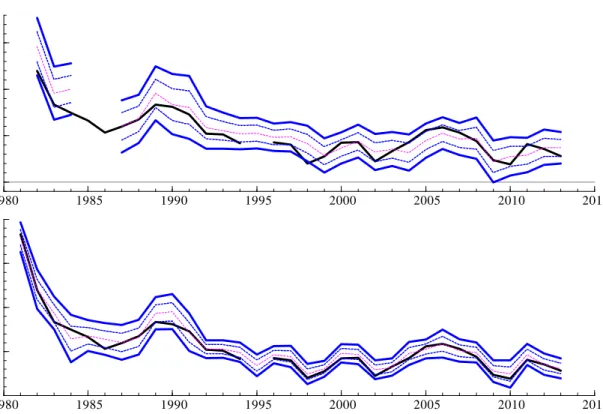
Figures 1 and 2 present a selective look-ahead to our results. For annual output growth and in‡ation, respectively, they present time series of the aggregate densities and the outcomes (advance estimates) for i) top panels, the year-ahead forecasts, made in response to the surveys held in the …rst quarters of the years 1982 to 2013, and ii) bottom panels, the one quarter-ahead forecasts, made in response to the surveys in the fourth quarters 1981 to 2013. Simply eye-balling the densities and the associated outcomes suggests short horizon forecasts are too dispersed: realizations outside the 80% interval (de…ned by the 90th and 10th percentiles) should occur a …fth of the time, but there are no such instances for output growth or in‡ation. Moreover, realizations outside the interquartile range should occur half the time. For output growth, from around 2000 onwards it appears that the actuals are well within the interquartile range much of the time, and for in‡ation occurrences outside the IQ range are rare. There are limitations to what can be learnt from a graphical analysis, and in the paper we provide formal assessments, and comparisons to benchmark forecasts, as well as an analysis of the individual forecasters.

We regard the value of survey macro-forecasts as established in the case of …rst-moment prediction, but as unproven in terms of the probability assessments implied by the histogram forecasts.

The remainder of the paper is as follows. Section 2 reviews the literature on forecast density evaluation, and on comparisons between forecast densities. Section 3 describes the survey data. Section 4 describes the construction of the benchmark densities, used to gauge the value of conditioning on forecast origin information. The results are given in section 5. Section 6 assesses the robustness of our main …ndings to the assumptions which have been made, and includes a section considering a number of alternative density scoring rules. Section 7 considers a simple correction based on the past performance of the SPF densities, which delivers more accurate densities over the out-of-sample period. Section 8 concludes.

2

The Evaluation of Survey Density Forecasts, and Comparisons

to Benchmarks

A popular way of evaluating survey density forecasts is based on the probability integral transform, dating back at least to Rosenblatt (1952), with recent contributions by Shephard (1994), Kim, Shephard and Chib (1998) and Diebold, Gunther and Tay (1998). Dieboldet al. (1998) and Granger and Pesaran (2000) show that a density forecast that coincides with the ‘true’forecast density will be optimal in terms of minimizing expected loss irrespective of the form of the (generally unknown) user’s loss function. In some applications only a portion of the forecast density may be relevant, as for example in …nancial risk management, where the tail quartile of the expected distribution of returns plays a prominent role (in Value at Risk calculations), or in macro in‡ation forecasting, where the focus is on the probability that in‡ation will exceed a target value. Tools have been developed for the study of quartiles and for events derived from density forecasts (see, e.g., Engle and Manganelli (2004), Clements (2004), Gneiting and Ranjan (2011) and Diks, Panchenko and van Dijk (2011)). Our focus is on the whole density but we also look at a particular region of the density, which correspond to lower than normal growth of real GDP, and rates of in‡ation close to the target value of 2%.

There are two parts to our empirical investigation of the forecast densities. In the …rst part, we assess how well the SPF forecast densities approximate the true, unknown densities, using the probability integral transform, and in particular, the extension due to Berkowitz (2001). In the second, we compare the SPF densities to the benchmark densities. Hence the SPF densities may be mis-speci…ed - of interest is whether they are nonetheless superior to the benchmarks. These comparisons are motivated by Lee, Bao and Saltoglu (2007) and Mitchell and Hall (2005), and the recognition that the Kullback-Leibler Information Criterion (Kullback and Leibler (1951), KLIC) measure of the divergence between a forecast density and the true density can be adapted to compare two or more densities, without making the assumption that any of the densities is correctly-speci…ed. The KLIC will be used to compare the SPF densities against the benchmark densities in the form of a Diebold and Mariano (1995) test of equal predictive ability, and amounts to a comparison in terms of logarithmic score. The testing of rival density forecasts is formalized by Amisano and Giacomini (2007) for a class of scoring rules, and their approach is shown to be valid when the densities are generated from mis-speci…ed models with estimated parameters, and when the resulting densities are dynamically mis-speci…ed. As well as considering the logarithmic score (henceforth log score) which is perhaps the most popular loss function of scoring rule for densities,2 we assess the robustness of our …ndings to the quadratic and ranked probability scores.

The benchmark densities are such that the rejection of the null of equal density accuracy in favour of the SPF densities would imply that the conditioning on the forecast origin information implicit in the survey

forecasts results in the superior accuracy.3 _{One would expect the forecast origin information would become}

less valuable for determining the scale of the forecast density as the forecast horizon increases. By considering density forecasts with horizons from approximately one quarter to one year ahead, it might be possible to determine the horizon at which the survey forecasts become ‘uninformative’, in the sense that, evaluated by KLIC, the conditioning information yields no improvement in accuracy.4

2.1

Density evaluation

Suppose we have a series of 1-step forecast densities for the value of a random variable _fYtg, denoted by

pY;t 1(y), wheret= 1; : : : ; n. The probability integral transforms (p.i.t.’s) of the realizations of the variable

with respect to the forecast densities are given by:

zt=

yt

Z

1

pY;t 1(u)du PY;t 1(yt) (1)

for t = 1; : : : ; n, where PY;t 1(yt)is the forecast probability of Yt not exceeding the realized value yt. In

terms of the random variables _fYtg, rather than their realized values fytg, we obtain random variables

denoted by_fZtg: Zt= Yt Z 1 pY;t 1(u)du PY;t 1(Yt):

When the forecast density equals the true density, fY;t 1(y), it follows by a simple change-of-variables

argument thatZt U(0;1), whereU(0;1) is the uniform distribution over(0;1). Even though the actual

conditional densities may be changing over time, provided the forecast densities match the actual densities at eacht, thenZt U(0;1) for each t, and the Zt are independently distributed of each other, such that

the realized time series_fztgnt=1 is an iid sample from aU(0;1) distribution.

This suggests we can evaluate whether the conditional forecast densities match the true conditional densities by testing whether _fztgnt=1 is iidU(0;1). Berkowitz (2001) suggested taking the inverse normal

CDF transformation of the_fztgnt=1series, to give, say,fztg n

t=1, on the grounds that more powerful tools can

be applied to testing the null that the_fz_tgn_t=1 are iidN(0;1) (forh= 1) compared to one of iid uniformity of the original _fztgnt=1 series. He proposes a one-degree of freedom test of independence against a

…rst-order autoregressive structure, as well as a three-degree of freedom test of zero-mean, unit variance and independence. In each case the maintained assumption is that of normality, so that standard likelihood ratio tests are constructed using the gaussian likelihoods.

3_{In a similar vein, for point forecasts Diebold and Kilian (2001) suggest measuring predictability by comparing the expected}

loss of a short-horizon forecast to a long-horizon forecast. We use the unconditional density as the ‘long-horizon’forecast, against which the SPF density forecasts are compared as the ‘short-horizon’forecasts. Note that our primary benchmark forecasts are unconditional in terms of the dispersion about the mean, but the mean is conditioned on forecast origin information. As noted in the text,trulyunconditional benchmarks are found to be clearly inferior.

4_{The way in which this discussion is framed assumes that the one-quarter ahead survey forecasts will outperform, and that}

The Berkowitz (2001) three degree of freedom test is given by:

LRB = 2(L(0;1;0) L ^;^2;^ ) (2)

where L(0;1;0) = Pn_t=1hln z_{tjt 1} i is the value of the Gaussian log-likelihood for an independently distributed standard normal random variable ( (:)is theN(0;1)pdf), and:

L ^;^2;^ = n X t=1 h ln z_{tjt 1} ^ ^z_{t 1jt 2} =^ =^ i

is the maximized log-likelihood for an AR(1) with Gaussian errors (_b’s on parameters denote maximum likelihood estimates). As noted by Lee et al.(2007), the assumptions of a …rst-order process, and that it is Gaussian, can be generalized: they allow instead a higher-order autoregression, with iid disturbances that follow a semi-non-parametric density function. However, for quarterly macro data relatively short-sample sizes perhaps warrant the simpler assumptions.

Finally, Knüppel (2015) suggests a simple way of testing whether thez are standard normal using the non-standardized, non-central (i.e., ‘raw’) moments of thez , and compares this approach with that of Bai and Ng (2005). We report tests of raw moments for the two moments, and for the …rst four moments.

2.2

Density comparison

Lee et al. (2007) show that the Berkowitz test can be interpreted as a particular form of KLIC-based evaluation of a forecast density compared to the true density, and that the KLIC can also be used to compare (two or more) mis-speci…ed identities.

Firstly, comparing a forecast density to the true density. The KLIC is de…ned as:

KLICtjt h=E[ln (fY;t h(yt)) ln (pY;t h(yt))]

where the expectation is with respect to the true density, so that:

KLICtjt h= Z fY;t h(yt) ln (fY;t h(yt)) (pY;t h(yt)) dyt:

Berkowitz (2001, Proposition 2, p.467) shows thatln (fY;t h(yt)) ln (pY;t h(yt)) = lnqZ ;t h(zt) ln (zt),

whereqZ ;t his the true (unknown) density ofzt and is the standard normal. The KLIC is estimated as

the sample average ofdtjt h lnqZ ;t h(zt) ln (zt)(overt, for a givenh), and if we allow thatzt is a

KLICh = 1 n n X t=1 dtjt h= 1 n n X t=1 h ln z_{tjt h} ^ ^z_{t 1jt h 1} =^ =^ i 1 n n X t=1 h ln z_{tjt h} i = (2n) 1LRB; (3)

where LRB is given in (2). Hence the KLIC and Berkowitz test are directly related. The assumption that

thez_{tjt h}are independent for optimal density forecasts is valid in our framework, as explained below. The KLIC can also be used as the loss function in a comparison of two density forecasts, using the approach to testing equal predictive accuracy of Diebold and Mariano (1995). Letting the loss di¤erential between the KLICs of the two densities bedtjt h, then

dtjt h = ln (fY;t h(yt)) ln p2Y;t h(yt) ln (fY;t h(yt)) ln p1Y;t h(yt) (4)

= ln p1_{Y;t h}(yt) ln p2Y;t h(yt) ;

wherep1()andp2()denote rivals sets of forecast densities. The average loss di¤erential is:

dh= 1 n n X t=1 dtjt h

with limiting distribution:

p

n dh E dtjt h

d

!N 0; 2 (5)

where 2 is the limiting variance.

We will use (5) to compare the SPF forecasts (say, p1

Y;t h) against the benchmark forecasts (p2Y;t h).

In which case, under the null of equal accuracy, E dtjt h = 0, and 2 = 0+ 2

P1 j=1 j, with j = E dtjt hdt jjt j h , and (5) is simply: dh =pn d !N(0;1): (6)

As noted in section 2, this corresponds to the approach to comparing density forecasts of Amisano and Giacomini (2007). The Amisano and Giacomini (2007) approach allows for comparisons between mis-speci…ed densities. This is important given that both the SPF and benchmark densities are found to be mis-speci…ed at the shorter horizons, and for this reason it might be important to allow for dynamic mis-speci…cation in the construction of the denominator of (6), as shown.

Note that we evaluate the forecast densities separately for each horizon, and the timing of the forecasts (explained in the next section) is such that the forecasts are non-overlapping. They are non-overlapping in the sense that the realization for the previous year’s Q1 survey forecast (say) is known before this year’s Q1 survey forecast is made. Hence for correctly-speci…ed forecasts, we would expect to be able to set _i= 0for

choose to use an autocorrelation-consistent estimator of the variance. 5

3

Forecast data description

We use the quarterly US Survey of Professional Forecasters (SPF) respondents’probability distributions for in‡ation and output growth. The SPF began as the NBER-ASA survey in 1968:4 and runs to the present day: see Croushore (1993). It has been extensively used for academic research into the nature of expectations formation: see https://www.philadelphiafed.org/research-and-data/real-time-center/survey-of-professional-forecasters/academic-bibliography.

We use the forecast distributions (provided in the form of histograms) from the 130 quarterly surveys from 1981:Q3 to 2013:Q4, inclusive, as our primary source of data.6 _{Over this period, the survey provides}

respondents’ histograms for output growth and in‡ation, in terms of the percentage change in the year of the survey relative to the previous year.7 _{For surveys which take place in the …rst quarters of the year, the}

latest available GDP and GDP de‡ator data are advance estimates for the fourth quarter of the previous year, so the forecast horizon is e¤ectively 4-quarters ahead. The next quarter - the second quarter of the year - the target is again the annual calendar year growth rate of the current year relative to the previous year, but now the …rst quarter advance estimates of the national accounts data are known, and the forecast horizon is 3 quarters. The shortest horizon therefore occurs for fourth quarter surveys, where there is data on all but the fourth quarter of the year.

We suppose that the forecasters are implicitly targeting an early vintage release. That is, the distributions are compared to the advance estimates of calendar-year output growth and in‡ation released in Q1 of the year following the year being forecast. 8 _{To be explicit, the actual calendar-year percentage growth rate (for}

GDP or its de‡ator) for the 1981:Q3 survey is given by:

100 Y 82:1 81:1 +Y81:282:1+Y81:382:1+Y81:482:1 Y82:1 80:1 +Y80:282:1+Y80:382:1+Y80:482:1 1 (7)

where Y refers to the (non-logged) value of the variable in the quarter given by the subscript, from the data vintage given by the superscript. The superscript here makes clear that all the data come from the 1982:Q1 vintage. The numerator is the sum of the quarterly values of the variable in the current year, and the denominator is the same for the previous year, where the current and previous year are relative to

5_{When we do so, we use the standard approach and estimate} 2 _by ^2 _where^2 _{= ^} 0+ 2 Pp j=1 p j p ^j, where ^0 = 1 n Pn t=1 dt d 2 ,^j= 1n Pn t=j+1 dt d dt j dj , anddt dtjt h,d=n1 Pn t=1dt,dj= _n1_jPnt=j+1dt j.

6_{The data were downloaded in December 2015, from}

http://www.philadelphiafed.org/research-and-data/real-time-center/survey-of-professional-forecasters/

7_{Also provided are histograms for the year-on-year calendar growth rates for the next year relative to the year of the survey,}

but we do not analyze these.

8_{These are taken from the quarterly Real Time Data Set for Macroeconomists (RTDSM) maintained by the Federal Reserve}

Bank of Philadelphia: see Croushore and Stark (2001). This consists of a data set for each quarter that contains only those data that would have been available at a given reference date: subsequent revisions, base-year and other de…nitional changes that occurred after the reference date are omitted.

the year the survey is held in. In order to forecast the calendar-year growth rate given by (7), the survey respondent will need forecasts of the remaining quarters of the current year, Y81:3 and Y81:4. Estimates of

the earlier two quarters of 1981 are available, but these are the 1981:Q3 vintage estimates, and are subject to revision relative to the 1982:Q1 vintage values used to generate the actual growth rate given by (7). (This also applies to the estimates of the 1980 calendar year values.) One would expect the e¤ects of the revisions to the ‘known-quarters’(Y81:2,Y81:1,Y80:4, ...,Y80:1) to be of secondary importance relative to the errors in

forecasting the future quarters.

The target remains the same for the 1981:Q4 survey forecasts, and now the only unknown Y81:4, so

intuitively there is less uncertainty about the calendar-year growth rates than in the previous quarter.9

The next quarter, 1982:Q1, the target switches to the 1982 calendar year growth, and remains so for the 1982 quarter surveys, and so on.

The sample begins with the 1981:Q3 survey, because prior surveys asked for probability distributions for nominal (as opposed to real) output. In fact there are a number of other complicating factors, to do with changes in variable de…nitions (GNP to GDP), base year changes, the size and locations of the histogram bins, the number of respondents, and the years to which the forecasts refer.10

The survey also provides point forecasts of the calendar-year GDP and the GDP de‡ator, which match the histograms in that they are …xed-event (see, e.g., Nordhaus (1987)) - forecasts of the same target (here, the annual calendar year growth rates) made at a number of forecast origins (here, the 4 surveys of the year). Rolling-event forecasts of GDP and its de‡ator are also made. These are forecasts of the values of the variables in the current and each of the next four quarters. These forecasts will be used in conjunction with the real-time data set to construct the benchmark densities, as described in section 4. We are able to use the rolling-event (or ‘…xed-horizon’) point forecasts from surveys prior to 1981:Q3. Although the output forecasts prior to 1981:Q3 originally referred to nominal GDP (GNP), forecasts of real GDP (GNP) have been constructed by the survey administrator using the forecasts of the de‡ator.

The probability assessments are reported as histograms, which provide an incomplete estimate of the densities. We …t normal distributions to the histograms (see, e.g., Giordani and Söderlind (2003, p. 1044) and Boero, Smith and Wallis (2015)) when there are 3 or more bins with non-zero probability attached, and otherwise we …t triangular distributions, in precisely the same way as explained in Engelberget al.(2009, see p.37-8). From these distributions we obtain estimates ofzand log scores. In order to do so, we follow much of the literature and assume the open-ended exterior bins are in fact closed, by assuming they have the same

9_{This is formalized by Manzan (2016) within a Bayesian framework in which an individual updates her/his prior density as}

new information becomes available.

1 0_{See, for example Diebold, Tay and Wallis (1999), Clements (2010) for a discussion of some of these aspects, as well as the}

online documentation provided by the SPF at https://www.philadelphiafed.org/research-and-data/real-time-center/survey-of-professional-forecasters. Many of these potential complicating factors can be readily dealt with, e.g., we omit the 1985:Q1 and 1986:Q1 since there is some doubt as to the years to which the survey histogram questions refer. Others, such as the changing composition of the ‘panel’ of forecasters potentially have more wide-reaching e¤ects. For example, we assume that data are missing ‘at random’ so that the sample is representative of the population. That is, failure by an individual to respond to a given survey occurs for reasons unrelated to the issues of interest in our study. López-Pérez (2015) is one of the few studies to consider whether the decision to participate is related to (say) perceived uncertainty about the outlook.

width as the interior bins. This assumption is innocuous when most if not all of the probability is assigned to inner bins, but matters when the location of the bins lags developments in the economy, resulting in a pile up of probability in an open bin, and e¤ectively a truncated distribution. This only appears to have been a potential problem for output growth in the 2009:Q1 and Q2 surveys for the SPF. In 2009:Q1 the aggregate histogram assigned a 34% chance to (2009-calendar-year) growth being less than -2. For the 2009:Q2 survey, a new lower bin was added, ‘< 3’, and the aggregate histogram indicated a 24% chance of this event. But as noted by Manzan (2016), there are no other quarters where a large average probability is assigned to an open interval, so that any distortionary e¤ects are likely to be minor (and have no e¤ect on the Q3 and Q4 survey forecasts). In contrast, Manzan (2016) shows that the problem is more acute for the European Central Bank SPF, and suggests …tting ‘arti…cial’triangular distributions, based on the assumption that an individual’s point prediction can be regarded as an estimate of the mode of his/her underlying distribution. Finally, as explained in this section, the SPF histogram forecasts are …xed-event, in that there are a number of forecasts of the same target of di¤erent horizons, e.g., forecasts of the 2010 calendar-year growth rate made in each of the four quarters of 2010. Then the 2011:Q1 survey targets the 2011 calendar-year growth rate, as do the remaining quarters of 2011, and so on. This has the major advantage for our purposes of delivering series of annual forecasts of horizons of 1, 2, 3 and 4 quarters ahead. It allows a study of the term structure, and the behaviour of the histograms as the horizon shortens. 11 The European Central Bank SPF provides both …xed-horizon 1-year ahead and 2-year ahead annual growth rate histogram forecasts, as well as …xed-event histogram forecasts, but many of the studies of the ECB-SPF use the medium or long-term …xed horizon forecasts (e.g., Abel, Rich, Song and Tracy (2016) and Kenny, Kostka and Masera (2014, 2015)) and are silent about the short-horizon properties of the forecasts.

4

The benchmark density forecasts.

Our benchmark density forecasts (BMs) are constructed from the historical distributions of past median SPF point prediction forecast errors. We centre the densities on the median point predictions of the annual year-on-year growth rates, in which case the BM densities condition on the location, but not the scale of the distribution. We use the median, as opposed to the mean of the cross-section of point forecasts, because the median is usually taken to be the consensus. We also calculate truly unconditional BMs, as explained below. In either case, the key input is the set of rolling-event forecasts of the quarterly values of horizons up to 4-quarters ahead. These forecasts are used to constructex ante, real-time distributions of forecast errors that are comparable to the errors in forecasting the calendar-year annual growth rates. We require: (i) that the forecast horizons match, and (ii) that the targets match. We explain how this is achieved by way of an example.

1 1_{D’Amico and Orphanides (2008) propose a way of constructing approximate 1-year …xed horizon forecasts for the US SPF}

Consider the construction of the benchmark density for the 1981:Q3 survey. The histogram forecasts made in response to this survey are 2-quarters ahead (in the sense that the latest data values for output growth or in‡ation are for 1981:Q2). Hence we need 2-step ahead forecast errors to construct the BMs. They must also be of the annual growth rate relative to the previous year. We calculate 50 2-step ahead annual growth rate forecast errors, using the 1968:Q4 survey to the 1981:1Q1 survey, inclusive. That is, the forecast errors would have been known at the time, so a density based on these errors could in principle have been constructed, and used to forecast. In this sense the benchmark density forecasts are real time.

The …rst of the 50 forecast errors is given by:

A ctual Value z }| { 100 Y 81:3 81:2 +Y81:181:3+Y80:481:3+Y80:381:3 Y81:3 80:2 +Y80:181:3+Y79:481:3+Y79:381:3 1 Forecast Value z }| { 100 F 81:1 81:2 +F81:181:1+Y80:481:1+Y80:381:1 Y81:1 80:2 +Y80:181:1+Y79:481:1+Y79:381:1 1 (8) where Fo

q refers to the forecast of target quarter q made at time (forecast origin o), and as in section 3,

Yv

q refers to the actual value of the variable in quarterq taken from data vintage v. The following points

should be noted: 1) the actual value is the value of the four quarters through 1981:Q2 as a percentage of the previous four quarters, all taken from the 1981:Q3 vintage of data; 2) ‘the’forecast consists of forecasts of two quarters, 1981:Q2 and 1981:Q1, both from the 1981:Q1 survey, and data values for the previous six quarters12; 3) the denominators in the Actual and Forecast growth rates refer to the same quarters (i.e., subscripts match), but the superscripts di¤er - for the Forecast value the actuals in the denominator come from the then available (1981:Q1) vintage.

The second of the …fty forecast errors (used to construct the benchmark density for the 1981:Q3 survey) is as (8) but based on a two-step ahead ‘year-on-year’forecast from the 1980:4 survey, that is:

A ctual Value z }| { 100 Y 81:2 81:1 +Y80:481:2+Y80:381:2+Y80:281:2 Y81:2 80:1 +Y79:481:2+Y79:381:2+Y79:281:2 1 Forecast Value z }| { 100 F 80:4 81:1 +F80:480:4+Y80:380:4+Y80:280:4 Y80:4 80:1 +Y79:480:4+Y79:380:4+Y79:280:4 1 (9)

Continuing back in time in this way results in the 50th forecast error being of the four quarters up to and including 1969:Q1, relative to the four quarters through 1968:Q1, all taken from the 1969:Q2 vintage, compared to the forecast of this quantity. This comprises forecasts from the 1968:Q4 survey of 1969:Q1 and 1968:Q4, and values of 1968Q3 and Q2 from the 1968:Q4 data vintage.

To generate a BM to match a fourth quarter survey density (such as 1981:Q4, to make things concrete), the forecast errors need to re‡ect the fact that there is one fewer quarter to forecast. The …rst forecast error is constructed as:

1 2_{The SPF provides ‘forecasts’ of the previous quarter’s value, and these are invariably set equal to the released data, i.e,}

A ctual Value z }| { 100 Y 81:4 81:3 +Y81:281:4+Y81:181:4+Y80:481:4 Y81:4 80:3 +Y80:281:4+Y80:181:4+Y79:481:4 1 Forecast Value z }| { 100 F 81:3 81:3 +Y81:281:3+Y81:181:3+Y80:481:3 Y81:3 80:3 +Y80:281:3+Y80:181:3+Y79:481:3 1 (10) and the second as:

A ctual Value z }| { 100 Y 81:3 81:2 +Y81:181:3+Y80:481:3+Y80:381:3 Y81:3 80:2 +Y80:181:3+Y79:481:3+Y79:381:3 1 Forecast Value z }| { 100 F 81:2 81:2 +Y81:181:2+Y80:481:2+Y80:381:2 Y81:2 80:2 +Y80:181:2+Y79:481:2+Y79:381:2 1 (11) and so on.

To generate BM densities to match …rst quarter survey densities, all the quarters in the numerator of the year-on-year growth rate forecast will need to be replaced by forecast values.

In all relevant respects the forecasts underlying the errors in (8) to (11) mirror the corresponding his-togram forecasts, and so the distribution of these forecast errors can be used as a valid benchmark for comparison. We …t normal distributions to these. For example, the 1981:Q3 truly unconditional distribu-tion is assumed to be normal with mean given by the average of the past forecasts, and variance given by the sample variance of the past forecast errors. Because the forecasts used to calculate the forecast errors are overlapping, we use an autocorrelation-correction. Speci…cally, we setp= 5 in the footnote to section 2.2. For the benchmark forecasts that condition on the location, we set the mean to the median SPF point prediction of the rate of growth of 1981 over 1980 made in response to the 1981:Q3 survey, and calculate the variance as for the truly unconditional densities. Fitting a normal facilitates the calculation ofz as well as the log score for comparison to the SPF histogram-based distributions.13

Our choice of benchmark forecasts are motivated in part by Rossi and Sekhposyan (2015). They use the empirical distribution of SPF forecast errors to construct an uncertainty index, based on the percentile of the historical distribution which corresponds to the forecast error for the particular realization: forecast errors in the tails are deemed more uncertain than those away from the tails. Our focus is di¤erent, but nevertheless past SPF forecast errors provide distributions against which the SPF conditional distributions can be compared.

5

Empirical Results

5.1

The Aggregate Distributions

Aggregate distributions calculated by equal weighting of the individual respondents’ forecast distributions are often the object of the analysis. Equal weighting is known in the literature as the linear opinion pool

1 3_{We do not need to assume normality to calculatez(and hencez ): we could simply look at the proportion of the historical}

errors which are less than the realization. However, when this is 0or 1, the calculation of z is problematic as the inverse normal cdf is not de…ned.

(see Genest and Zidek (1986)), and such forecasts are reported by the US SPF along with the individual histograms, although there are other ways of combining density forecasts (Hall and Mitchell (2009) provide a review). Denoting individuali’s density forecast forYtmade at timet hbypY;i;t h(yt), with mean and

variance _{i;tjt h}=R1₁ytpY;i;t h(yt)@ytand 2_{i;tjt h}=R1₁(yt it)

2

pY;i;t h(yt)@yt, fori= 1; : : : ; N the

aggregate density is: pY;t h(yt) =_N1 PN_i=1pY;i;t h(yt)with mean and variance given by:

tjt h =N1 N X i=1 i;tjt h 2 tjt h = 1 N N X i=1 2 i;tjt h+ 1 N N X i=1 i;tjt h tjt h 2 : (12)

Hence the mean of the aggregate distribution is the simple average of the means of the individual distribu-tions, whereas the variance is the average of the individual variances plus the second term which measures disagreement between forecasters, and serves to increase the aggregate variance relative to the cross-section average: see Wallis (2005), extending earlier work by e.g., Lahiri, Teigland and Zaporowski (1988).

Use of the aggregate histograms allows unbroken sequences of forecasts across the entire sample, as the average is taken across all respondents (with ‘N’varying overt), and the changing composition is ignored. For many individuals there are many non-response surveys, generally due to late joining or leaving the survey, which is obviously exacerbated by the survey’s long historical duration (relative to similar surveys, such as those run by the ECB and Bank of England, for example). The aggregate histograms are often regarded as a summary measure of the information in the survey, in much the same way as the median point prediction is often taken as the survey point prediction, and used in comparisons with model forecasts, for example. But whereas the average point prediction is a ‘good’ summary measure (see, e.g., Clemen (1989), Aiol…, Capistrán and Timmermann (2011) and Manski (2011) as examples of a very large literature), the same may not be true of density combination because of the in‡ation of the variance of the aggregate histogram (relative to, say, a randomly-selected individual histogram). We address this issue below by using a measure of the average variance which abstracts from the disagreement term in (12).

The aggregate histograms always allocate non-zero probability to more than 2 bins, so that the normal distribution is …t to all the histograms, and is used to calculatez and the log scores.14

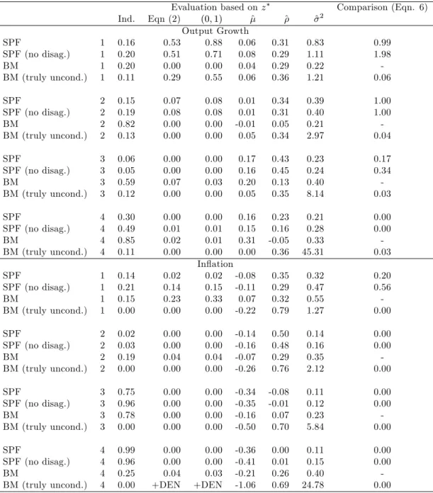
The results are recorded in table 1. Consider …rst the SPF densities (not ‘corrected’ for the e¤ects of disagreement) - these are the …rst rows for each forecast quarter headed simply by ‘SPF’. For the Q1 surveys (corresponding to a 4-quarter ahead horizon) the output growth forecasts are not rejected using any of the three Berkowitz tests, but the output growth densities are rejected for the three other survey quarters (so for forecast horizons of 3, 2 and 1 quarters ahead). The SPF in‡ation forecast densities are rejected for all survey quarters. As noted above, a possible explanation of the rejection of the aggregate SPF forecasts is

1 4_{When, as here,zis calculated after …tting a Gaussian distribution to the histogram, taking the inverse standard normal}

cdf ofzto givez results inz = (y ^)=^, whereyis the realization, and ^and ^2are the mean and variance of the …tted distribution.

that disagreement in‡ates the variances of the aggregate histograms, leading to the histograms being ‘too dispersed’ given the realizations, and thez variables showing too little dispersion: this is consistent with the estimates of the variances of the AR(1) model …t to_fz_tg reported in table 1. One way of dealing with this concern is to simply calculate the variance of the aggregate histogram as the cross-sectional average of the individuals’ histogram variances, setting the second term in (12) to zero.15 _{The results of doing so}

are recorded in the rows headed ‘SPF (no disag.)’. There is no change regarding inference based on the Berkowitz tests at the 5% level. There are some minor changes, mainly at the longer horizons. For example, the Q1 in‡ation densities are no longer rejected at the 1% level on the 2 and 3-degree of freedom Berkowitz tests (but they would be at the 2% level).

The results of the raw moment tests of Knüppel (2015) also suggest the SPF densities are inadequate. The test that the z are standard normal based on the …rst four raw moments (column headed ‘First 4’) rejects the Q1 survey output growth forecasts: of all the SPF forecasts, only the Q1 output growth forecasts corrected-for-disagreement are not rejected.

Next, we consider the adequacy of the two sets of Benchmark forecasts. Except at the longest-horizon …rst-quarter surveys, the adequacy of these forecasts is resoundingly rejected. For in‡ation, the …rst quarter Benchmark forecasts (which condition on location, denoted simply ‘BM’ in the table) are not formally rejected on any of the 3 Berkowitz tests at the 5% level, but the unconditional Benchmark (‘BM (truly uncond.)’) is rejected for in‡ation. For output growth, and the …rst quarter surveys, we …nd the reverse.

Having found all densities (SPF and the Benchmarks) mis-speci…ed on the Berkowitz tests for all but the longest horizon forecasts, what can we say about the relative comparison of the SPF against BM (on log score)? The …nal column of the table reports comparisons of the forecast densities against BM based on KLIC (or log scores) using equation (6). The entries in the tables are constructed such that a value less than 0.05 leads to a rejection of equal accuracy in favour of the BM at the 5% level (one-sided test), and an entry greater than 0.95 rejects in favour of the alternative (SPF, SPF (no disag.) or BM (truly uncond.)) being more accurate (at the 5% level in a one-sided test). The aggregate SPF are more accurate at the two longer horizons (the …rst two quarters of the year) for output growth, no better or worse for third quarter surveys, and less accurate at fourth quarter surveys. For in‡ation, the SPF are no better at the longest horizon, but worse at the other three shorter horizons.

Moreover, the comparison of the two sets of Benchmark densities for both variables and for all survey quarters clearly favours the BM forecasts which condition on location.16 _{For both variables and all survey} 1 5_{In fact we calculate the standard deviation of the aggregate histogram as the average of the individuals’standard deviations.}

The results of doing so are indistinguishable from taking the square root of the average of the individuals’variances. Abelet al.

(2016) calculate the ‘average variance’ by …rst estimating the variance of the aggregate histogram, and then subtracting the disagreement term. See also Lahiri and Sheng (2010) and Lahiri, Peng and Sheng (2015).

1 6_{Including for the …rst-quarter output growth forecasts, that is, notwithstanding the failure to reject the unconditional}

Benchmark densities on the Berkowitz tests, and the rejection of those which condition on location. The Berkowitz tests reject in part because the estimated variance ofz is less than 1 (^2 _{= 0:23for Q1 output growth forecasts). For the truly}

unconditional densities, the large forecast errors which result from not conditioning on location result in more extreme values ofz and an estimated variance close to1.

quarters we reject in favour of BM against the unconditional BM at the 5% level.

In summary, then, the survey densities fare worse as the forecast horizon shortens. For output growth the survey densities are only rejected at the shortest horizon, while for in‡ation the survey densities are rejected at all but the longest (4-quarter) horizon.

The results hold irrespective of how disagreement is treated. The reported results set the covariance terms to zero in the calculation of the asymptotic variance of the Diebold-Mariano statistic (6). The results did not change to any signi…cant degree if we used instead an autocorrelation-consistent estimator of the standard error.17

5.2

The Individual Distributions

We report results for all individuals who …led more than 15 forecasts of a given horizon. There is no requirement that these are made in consecutive years. We …t normal distributions when histograms have 3 or more non-zero bins, and (isosceles) triangular distributions when either one bin has all the probability mass, or it is distributed across two (adjacent) bins. Triangular distributions result in values of z of 0 or 1 when the realization falls outside of the support: these are arbitrarily set to 0:01and 0:99, respectively. (Then z = 2:3263 and is well de…ned, and an interpretation is that no realized values are viewed as ‘impossible’by the SPF respondents). We make the same assumption when we calculate log scores. However this assumption is arbitrary, resulting from the log score not being de…ned for outcomes with zero forecast probability. Boero, Smith and Wallis (2011) suggest the use of alternative scoring rules for histogram-based probability assessments, as such eventualities are likely to arise when forecasts are presented as histograms (see, also, Kenny et al.(2014)). We consider the use of alternative scoring rules arguably better suited to assessing histograms in section 6.4.

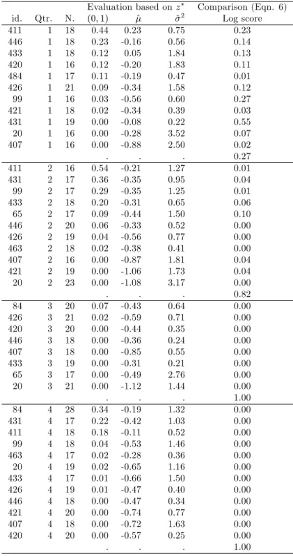
Tables 2 and 3 report results for output growth and in‡ation. We report a two-degree of freedom test of zero-mean and unit-variance, but do not allow an AR(1) as the unrestricted model because there are fewer observations for individuals, and because there are missing values, which would complicate the …tting of an autoregressive model. (Moreover, the results for the aggregate histograms suggest that power to reject the null is more likely to come from testing the mean and variance ofz , not from testing for autocorrelation). For each individual and horizon, then, we report the number of forecast observations, the p-value of the Berkowitz two-degree of freedom test, the estimates of the mean and variance, and the Diebold-Mariano test of the log scores. The results for individuals are sorted byp-value of the Berkowitz test within each survey quarter (equivalently, forecast horizon).

Consider table 2 for output growth. Except at the longest horizon, the statistical adequacy of the SPF densities is rejected for fewer than one third of respondents at the 5% level. (Speci…cally, for Q2, 2 of 12; for Q3, 2 of 9; and for Q4, 4 of 13). This suggests the scales of the individual respondents’histograms may be

better calibrated than the scales of the aggregate distributions, with two thirds of individuals reporting 1-quarter ahead (Q4 survey forecasts) which are well calibrated. However, the fewer rejections at the individual level may also re‡ect lower power due to the smaller sample sizes. Tellingly, the BM forecasts (conditioning on location) are statistically more accurate on log score than the forecasts of each individual SPF respondent at the shortest horizon (i.e., for Q4 surveys). (The entries in the table are constructed as in table 1, such that a value below 0.05 suggests the BM are more accurate at the 5% level (one-sided test), and an entry greater than 0.95 rejects in favour of the SPF being more accurate (at the 5% level in a one-sided test). At the longer horizons, the SPF forecasts are not rejected against the BMs (i.e., for the Q1 and Q2 survey quarters) but instances of rejecting in favour of an SPF respondent are rare. In summary, the comparisons against the BM forecasts suggests that the individual SPF output growth densities are poor at the shortest horizon.

For in‡ation (table 3) the rejection of the SPF forecasts is less equivocal, in that the SPF forecasts are rejected on the Berkowitz test for 7 out of 8 and 9 out of 12 respondents for Q3 and Q4 forecasts, respectively, and in addition, the forecasts of all these individuals are found to be statistically less accurate than the BM forecasts for most individuals except at the longest horizon, Q1 surveys.

6

Robustness of the results to the assumptions

We consider whether the …ndings discussed in section 5 are unduly dependent oni) the assumptions we have made in order to construct forecast densities from the histograms, andii) the use of log score as the density scoring rule, given that the probability assessments come from histograms.

6.1

The wider histogram bin widths before 1992:Q1.

Prior to 1992, respondents assigned probabilities to intervals of width 2 percentage points. From 1992Q1 onwards a …ner gradation was adopted with intervals being halved. The use of wide intervals may give a misleading picture when uncertainty is low, and all the probability is assigned to one interval. In such circumstances, a symmetric triangular distribution (with support on the full interval) results in a variance of0:0416when the interval width is one, but (four times as large) at0:1666when the interval width is two. Individuals are more likely to assign all the probability to one interval in response to Q4 surveys, because perceived uncertainty will be smaller at the shortest horizon. Hence our approach will place a ‡oor on the variance (and will a¤ect the z and log score calculations) for earlier-period one-bin histograms which may be particularly distortionary prior to 1992.

We tackle this in two ways.

Firstly, we approximate the one-bin histograms prior to 1992 by a symmetric triangular distribution with a base of one (rather than two), located centrally within the interval. There is no way of knowing whether this provides a more accurate representation of the underlying subjective distribution. We simply wish to

assess whether the way we treat the wide single-bin histograms is driving the results. This has no e¤ect on the aggregate results for either variable, because all the aggregate histograms allot probability to 3 or more bins. For individuals the change is most likely to a¤ect the shorter horizon forecasts. For the shortest horizon for output growth there are inconsequential changes. We still reject for 4 of the 13 respondents, and for all respondents reject in favour of the BMs on log score comparisons. (These results are not shown). The results for in‡ation are also unchanged.

Secondly, we set the beginning of the forecast sample to 1992:Q1. Some authors have regarded the post 1992 period of the SPF as providing cleaner forecast data under the stewardship of the Philadelphia Fed, and it avoids the drop o¤ in participation rates that occurred in the 1980s (see, e.g., Engelberget al.(2009) and Manzan (2016)). Curtailing the sample in this way has the drawback of discarding around a third of the observations, and reducing the number of individual respondents we can separately analyze, but also counters the potentially more insidious e¤ects of the wider bins not picked up by the …rst strategy. The aggregate histogram results for output growth and in‡ation are broadly unchanged, apart from the SPF output growth forecasts no longer being rejected for Q2 surveys (i.e., for h = 3) at the 5% level. Hence we continue to reject the SPF in‡ation forecasts being well speci…ed at all horizons, and the SPF output growth forecasts are rejected at the two shorter horizons. The pattern of results by individual is also largely unchanged. For Q4 surveys (h= 1) we …nd evidence against the forecasts being well speci…ed for 5 of 11 and 7 of 10 respondents for output growth and in‡ation, respectively, while for all these respondents we reject in favour of the BMs being more accurate.

6.2

Centreing the SPF densities on the point predictions.

Engelberget al.(2009) …nd inconsistencies between the central tendencies and the point predictions for some SPF respondents, and Clements (2010) …nds evidence that the point predictions tend to be more accurate in terms of traditional forecast evaluation criteria such as squared error loss. This raises the suspicion that the relatively good performance of the BMs may result from their being centred on the (cross-sectional) median point prediction. This turns out not to be the case. Centreing the SPF aggregate histograms on the median point predictions, and the individual histograms on the individuals’point predictions,18 _{does not result in a}

marked improvement in the SPF forecasts. (Results for the aggregate and individual densities are available in a Not For Publication Appendix).

6.3

Evaluating regions of the densities

Notwithstanding the poor performance of the short-horizon SPF forecast densities relative to the uncondi-tional benchmark evaluated on log score, the possibility remains that the SPF densities may fare better for

1 8_{For the individual respondent histograms with probability assigned to 3 bins or more, a normal density is …t to the histogram,}

as in the standard approach, and the estimated mean is then replaced by the individual’s point prediction. For the one and two bin histograms for which we assume triangular distributions no use is made of the point prediction.

particular regions of the density, such as the ‘event’de…ned by output growth being less than some threshold value, for example, or of in‡ation being in the vicinity of 2%.19

We might view the SPF output growth forecasts much more favourably if it were the case that the densities implied high forecast probabilities of declines in output when output did indeed fall.20 _{Or if the}

in‡ation densities were accurate for rates of in‡ation in the region of 2%. Because there were only three calendar years of negative annual growth during our sample, there are insu¢ cient observations of declines in output to reliably compare SPF and benchmarks densities in terms of this event. Instead, we consider slower than normal output growth, de…ned as annual growth less than 11₂%, or alternatively, less than2%. (These events occurred for 6 and 9 calendar years, respectively, so the number of observations underpinning the comparisons is still small). For in‡ation, we de…ne the region of interest as being11

2 2 1

2%, or1 3%

(occurring 10 and 22 times, respectively).

The region-speci…c tests of the densities we report are the KLIC-based comparisons of the conditional likelihood score functions of Dikset al. (2011, p.219, eqn (9)). That is, instead of comparing the log scores of the SPF and benchmark densities (as in equations (4) to (6)), the di¤erence between the log scores at timet is replaced by the di¤erence between the conditional likelihood scores. The log score for the density,

ln(pY;t h(yt)), is replaced by:

1 ( 1< yt< 2) ln

pY;t h(yt)

PY;t h( 2) PY;t h( 1)

whereP()is the cumulative distribution function corresponding to the densityp(), and1 ()is the indicator function (equal to1 when the argument is true, and zero otherwise), and 2 and 1 are the event-de…ning

thresholds, with 2> 1. For output growth, 1= 1, and 2 is either11₂%or 2%. For in‡ation, 1 and 2 are either 112,2

1

2 or f1,3g. Diks et al. (2011) also propose a censored likelihood approach, and we

could alternatively have used the approach of Gneiting and Ranjan (2011).

Table 4 compares the test results using log score (copied from Table 1) with those based on the conditional likelihood scores for the two events of interest for each variable. By and large, the di¤erences are small for both variables, for both events. We conclude that there is no evidence that SPF respondents are relatively better at forecasting regions of the densities corresponding to lower rates of growth of output, or to rates of in‡ation in the region of the2%target.

The similarities between the whole density …ndings and those for the events of interest also serve as a check of a sub-sample (that is, periods of lower rates of growth, or in‡ation close to 2%) against the whole sample. Further sub-sample analysis could be undertaken to check the constancy of the …ndings over time, but the nature of the forecast data is such that we only have a relatively small of observations at each horizon. That is, for a given horizon, we only have one forecast observation for each year of the survey.

1 9_{The 2% target was formally adopted by the FOMC at its meeting in January 2012, and was for the price index for personal}

consumption expenditures. See, e.g., https://www.federalreserve.gov/faqs/money_12848.htm.

6.4

Alternative density scoring rules

Notwithstanding the popularity of the log score in the literature, alternative scoring rules may be preferable for scoring probability forecasts presented in the form of histograms, as noted earlier. In this section we discuss alternative rules and why they may be preferable in our context, and assess the robustness of the results to the scoring rule used.

We consider the quadratic probability score (QPS: Brier (1950)) and the ranked probability score (RPS: Epstein (1969)), de…ned by:

QP S= 1 N N X t=1 K X k=1 pk_t yk_t 2 (13) and: RP S= 1 N N X t=1 K X k=1 P_tk Y_tk 2 (14)

where there are N forecasts (indexed byt), and for each forecast a probability is assumed to be assigned to each of the K bins (indexed by the superscriptk), denoted bypk

t. ykt takes the value1 when the actual

value is in bin k, and zero otherwise. In the de…nition of RP S, Pk

t is the cumulative probability (i.e.,

Pk

t =

Pk

s=1pst), and similarlyYtk cumulatesytk: Ytk= 1for all k s, where binscontains the actual value.

Being based on cumulative distributions, RPS will penalize less severely density forecasts with probability close to the bin containing the actual, relative to QPS. For QPS, a given probability outside the bin in which the actual falls has the same cost regardless of how near or far it is from the outcome-bin. 21

The notation used in (13) and (14) is deliberately simpli…ed, as we have suppressed the forecast horizon, the individual forecaster (or aggregate), and the fact that the number of bins K changes over time. As described above, QPS and RPS are expressed as loss functions, but in terms of the comparisons reported in the tables are calculated so as to be comparable to log score.

So, QPS and RPS are calculated directly from the SPF histograms using (13) and (14). For the benchmark forecasts, we use the normal distributions (assuming the mean is equal to the median of the cross-section of survey point predictions) that we have estimated from the historical forecast errors, and from these we estimate histograms, using the same number of bins, and location of bins, as underpins the matching SPF forecasts at that point in time. 22

Table 5 compares the results of testing the SPF histograms against the benchmarks using a Diebold-Mariano test for each of the three scores (the information for the log score repeats that in table 1 and is

2 1_{In addition, there is a further di¤erence between QPS and RPS given the way we treat the SPF de…nitions of the bin}

locations. Suppose the histogram has 100% probability in the SPF interval 6 to 7.9, and obviously 0% in all other intervals, such as the lower adjacent interval de…ned as 4 to 5.9. The realization is 5.9839. We assume the bins are de…ned as[4;6]and

[6;8], and since the realization is in the range (5.95 to 6.05), we assume the actual value is 6 and straddles the two bins. We setyk

t =

1

2 for these two bins. For QPS, then, the relevantp

k

t are0;1and theykt are

1 2, 1 2, so QPS is0:5. For RPS, theP k t

values are0;1(as forpk

t), butYtkis 12;1, and RPS is0:25.

2 2_{In terms of the example in the previous footnote, we evaluate the cdf for the given normal distribution at 8 and 6, and the}

shown for ease of comparison). Note that for the aggregate SPF histograms probability is assigned to 3 or more bins for both variables for all time periods, and so normal distributions are …tted to the histograms, and the issue of outcomes being assigned a non-zero probability can not arise. The broad picture for the aggregate histograms is not changed by using QPS or RPS in place of log score, in the sense that the shortest-horizon (Q4 survey) SPF forecasts are rejected against the Benchmark forecasts at the 5% level. However, a more detailed look suggests there are di¤erences - RPS does not reject the Benchmark forecasts at the longer horizons for output growth, and the Q4 RPS statisticp-value is now0:01. For in‡ation, there is no evidence against the SPF forecasts on QPS or RPS at the longest horizon.

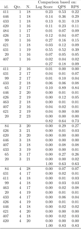
The use of QPS and RPS cast the individual SPF forecasters in a more favourable light in terms of output growth, compared to log score: see table 6. For the Q1 and Q2 surveys, few if any SPF individuals’forecasts are rejected (at the 5% level). Whereas on log score nearly a half of the forecasters, and all the forecasters, are rejected in terms of their Q3 and Q4 forecasts, respectively, the proportions rejected on QPS and RPS are markedly lower. Nevertheless, around 40 to 50% of forecasters density forecasts are rejected at Q4, the shortest horizon.23 _{For in‡ation (table 7) the use QPS and RPS suggest around two-thirds of respondents’}

Q3 forecasts can be rejected, as opposed to all respondents using log score, but at Q4 QPS and RPS are largely in line with log score.

7

Correcting the SPF aggregate density forecasts

Given that our …ndings appear relatively robust, we consider whether the SPF forecasts can be improved with simple mechanical corrections. Such corrections are commonplace in the point prediction forecasting literature, and are sometimes viewed as a way of ‘…xing’ a model’s forecasts for mis-speci…cation resulting from structural change (see, e.g., Castle, Clements and Hendry (2015)). It is possible to (re-)calibrate future forecast densities for the apparent mis-speci…cation of past densities (for which realizations are available): see, e.g., Dawid (1984), Kling and Bessler (1989) and Diebold, Hahn and Tay (1999). However, given the relatively small number of forecast densities of a given horizon, we consider whether a simple scaling of the SPF aggregate densities would improve their accuracy on log score. Based on the …rst 15 forecast densities (that is, the densities of 1982 to 1996 for the Q1 and Q2 surveys, or 1981 to 1995 for the Q3 and Q4 surveys), we calculate a horizon-speci…c scale factor that maximizes log score over this in-sample period,24 _{and then} 2 3_{The di¤erences between log score, and QPS and LPS, might be expected to be greatest for the shortest-horizon Q4 survey}

forecasts. Respondents will typically assign probability to fewer bins, re‡ecting the lower level of uncertainty about the future, and the problems of ‘zero-probability’ outcomes resulting from …tting triangular distributions will be more acute.

2 4_{Given a set of normal forecast densities de…ned by} t; 2t

N

t=1and realizationsfxtg

N

t=1, the log score is de…ned by:

PN t=1lnp xt; t; 2 t = PNt=1ln t 1 2 PN t=1ln 2 PN t=1 (xt t)2 2 2 t

Choosing to maximize the log score over1toN, where^2t = 2t:

PN t=1lnp xt; t;^2t = 1 2Nln PN t=1ln t 1 2Nln 2 1 2 PN t=1 (xt t) 2 2 t

apply these factors to the variances of the remaining, out-of-sample density forecasts.

Success would require that the variances of the SPF densities systematically over (or under) estimate the uncertainty over the in-sample period, and that the same remains true of the out-of-sample period. Table 8 records the results for the out-of-sample forecast densities 1996(1997) to 2013.

The …rst three rows of each panel give the average log scores for the out-of-sample period for the SPF densities, for the SPF densities with the variances scaled by the in-sample estimate of , denoted SPFc, and

for the BM densities. For the SPF densities we remove the impact of disagreement, and the BM densities are centred on the median point predictions. The DM test results of the (uncorrected) SPF against the BM for the out-of-sample period are similar to the full-sample results in table 1: for output growth the SPF densities are rejected against the BM for Q4 surveys (shortest horizon), and for in‡ation the SPF densities are less accurate for Q2 to Q4 surveys. Hence the truncation of the assessment period to allow an in-sample period to estimate does not a¤ect the …ndings regarding the SPF aggregate densities.

Table 8 shows marked improvements on log score from scaling-down the variances by the …xed in-sample factors, in all cases except the Q1 output growth forecasts. The improvements in log score result in the Q3 output growth forecasts now being superior to the BMs, and the Q2 SPF in‡ation forecasts not being rejected as less accurate than the BMs. Not withstanding the improvements in log score at the shortest horizon (Q4 survey quarter) forecasts, these densities are still rejected.

The estimates of suggest that the optimal in-sample variances are around a half of the survey variances (for all but the Q1 output growth densities). Applying these adjustments out-of-sample is clearly bene…cial, and in some cases changes the inference concerning the relative accuracy of the SPF and BM densities, as noted. That corrections based on past performance up to the mid 1990s yields improvements on average over the remainder of the 1990’s and the period up to 2013 suggests systematic failings in the SPF forecasts.

8

Conclusions

Other papers have considered the aggregate US SPF histograms, see, e.g., Diebold et al.(1999) and Rossi and Sekhposyan (2013). The novelty of the current contribution is the investigation of the term structure of the aggregate densities and those of individual survey respondents, and the comparison to the benchmark forecasts. The BM densities with means set equal to the median point prediction are designed such that the SPF densities would be superior were the respondents able to gauge the degree of uncertainty characterizing the macro-outlook at the time the forecasts are made.

Our …ndings suggest that the aggregate and individual forecast densities tend to be too dispersed at the shorter forecast horizons, such as one quarter and two quarters ahead, consistent with the …ndings of Clements (2014) in his study ofex anteandex post forecast uncertainty. Because of the excess dispersion of the survey densities at short horizons, the expected dominance of the SPF densities over the

variance benchmark distributions at short horizons does not materialize. The benchmark densities are rejected at short horizons on tests of correct speci…cation, as expected, given that the dispersions of these distributions are not conditioned on developments at the time the forecasts are made. However, the excess dispersion on the aggregate SPF densities renders these densities less accurate than the benchmarks on log score comparisons.

The rejection of the short-horizon density forecasts of output growth and in‡ation occurs for the aggregate densities irrespective of whether an allowance is made for disagreement and irrespective of whether we use log score, QPS or RPS as the scoring rule.

At the individual level, the use of QPS or RPS tends to cast the survey expectations in a more favourable light, compared to when log score is used. Even so, the output growth forecasts of two …fths of the re-spondents, and the in‡ation forecasts of four …fths of the rere-spondents, are rejected against the benchmark forecasts for the one-quarter ahead horizon.

Of course the forecasters’ subjective probability assessments at short horizons may well be driven by motives other than maximizing accuracy as judged by log score. The respondents’ loss functions may be such that the respondents are incentivized to ensure that realized outcomes fall well within the likely range of outcomes implied by their probability assessments, for example. Be that as it may, the excess dispersion of the aggregate histograms at short horizons is su¢ ciently large and persistent that the application of correction factors (based on a training sample of forecasts and realizations) to out-of-sample probability assessments leads to marked improvements in their (log score) accuracy.

Although we have considered a single macro-survey, it is the longest and probably most used in terms of the probability assessments it provides. Our …ndings question the reliability of the short-horizon survey densities.

References

Abel, J., Rich, R., Song, J., and Tracy, J. (2016). The Measurement and Behavior of Uncertainty: Evidence from the ECB Survey of Professional Forecasters. Journal of Applied Econometrics,31(3), 533–550. Aiol…, M., Capistrán, C., and Timmermann, A. (2011). Forecast combinations, chapter 11. In Clements,

M. P., and Hendry, D. F. (eds.),The Oxford Handbook of Economic Forecasting, pp. 355–388: Oxford University Press.

Amisano, G., and Giacomini, R. (2007). Comparing Density Forecasts via Weighted Likelihood Ratio Tests. Journal of Business & Economic Statistics,25, 177–190.

Andrade, P., and Le Bihan, H. (2013). Inattentive professional forecasters. Journal of Monetary Economics, 60(8), 967–982.

Ang, A., Bekaert, G., and Wei, M. (2007). Do macro variables, asset markets, or surveys forecast in‡ation better?. Journal of Monetary Economics,54(4), 1163–1212.