in partial fulfillment of the requirements for the degree of

(1)

Computer Aided Design and Synthesis

of the RSCR Spatial Mechanism

by

Jeffrey M. Thompson

Thesis submitted to the Faculty of the Virginia Polytechnic Institute and State University

in

partial fulfillment of the requirements for the degree of

Master of Science

m

Mechanical Engineering

APPROVED:

Dr. Arvid Mykle'1tst, Chairman

~--=-...,,:---=----,:--=--=-..,...,.~~·-~ Dr. Charles F. Reinholtz

April 28, 1987 Blacksburg, Virginia

(2)

Computer Aided Design and Synthesis

of the RSCR Spatial Mechanism

by

Jeffrey M. Thompson

Dr. Arvid Myklebust, Chairman

Mechanical Engineering

(ABSTRACT)

Recent efforts in computer aided design and computer aided manufacturing have

stressed the development of robotics. However, there are many applications where a

spatial mechanism could be used in place of a robot, but the mechanism design theory

has not been fully developed. This thesis presents the fundamentals of a computer aided

design system for the RSCR (revolute-spheric-cylindric-revolute) spatial mechanism.

Exact relationships for position, velocity, and acceleration analysis have been derived.

Closed form synthesis equations have been developed for the RS and RC dyads. The

theory developed in this thesis has been implemented on the digital computer in the form

of a FORTRAN77 computer program. This computer implementation includes

inter-faces with MECHIN, a graphical preprocessor for spatial mechanism synthesis and

analysis, and GENMOD, an automatic model generator for spatial mechanisms.

(3)

Acknowledgements

I would first like to express my gratitude to my advisor and major professor, Dr. Arvid

Myklebust for his guidance in the research and preparation of this thesis.

I also wish to thank Dr. Charles Reinholtz for his advice and suggestions.

I would also like to thank Dr. Hamilton Mabie for his service on my advisory

commit-tee.

I wish to thank my fellow M.E. graduate students for their help and suggestions. In

particular, I would like to thank Brian Thatch, Veeraraghavan Arun, Bob Williams,

Mitch Keil, and Harinder Singh Oberoi.

Last, and certainly not least, I would like to thank my parents, Joseph and Jean

Thompson, for their guidance and support throughout my education.

(4)

102

SUBROUTINE ANALIN . . . 102 SUBROUTINE ANGDIR . . . 104 SUBROUTINE BUILD . . . ... . . .

105

SUBROUTINE CROSS . . . 106 SUBROUTINE DEFMAT . . .

106

SUBROUTINE DETERM . . . 107 SUBROUTINE DOT ... 107 SUBROUTINE FNDMAT . . .

107

SUBROUTINE FNDVEL . . .

108

SUBROUTINE FXPVT . . . 108 SUBROUTINE LNKLEN . . . 109 SUBROUTINE MATVEC . . . 109 SUBROUTINE MODGEN . . . 110 SUBROUTINE PANDQ . . .

111

SUBROUTINE QUARTC . . .

111

SUBROUTINE RCDY AD . . . 113 SUBROUTINE RESTRT . . .

114

SUBROUTINE REVLOC . . . 118 SUBROUTINE ROTACC ...

118

SUBROUTINE ROTMAT ... 119 SUBROUTINE RSCRAN . . . 119 Table of Contents vi

(7)

SUBROUTINE RSDY AD . . . 123

SUBROUTINE SPHLOC . . . 124

SUBROUTINE SYNTH . . . 124

SUBROUTINE UNIT . . . 126

SUBROUTINE VECSUB . . . 127

SUBROUTINE VMAG . . . 127

SUBROUTINE VMA T . . . 127

SUBROUTINE WDTMAT ... 127

SUBROUTINE WMAT . . . 128

SELECTED MECHIN SUBROUl1NES . . . • . . . 129

PROGRAM MECHIN . . . 130

SUBROUTINE ANIN . . . 130

SUBROUTINE DATA . . . 131

SUBROUTINE MENU . . . 132

SUBROUTINE RSCRA . . . 137

SUBROUTINE RSCRS ... 140

SUBROUTINE SDATA · . . . 143

SUBROUTINE SMENU . . . 143

SUBROUTINE SYNIN . . . 146

SUBROUTINE WRANAL ... ; . . . 147

SUBROUTINE WRSYN . . . 147

RSCR MODIFIED FOR MECHIN . . . 149

SUBROUTINE RSCRB . . . 149

SUBROUTINE SYNTHB . . . 150

SUBROUTINE ANALIB . . . 151

(8)

Vita

. . .

153

(9)

List of Illustrations

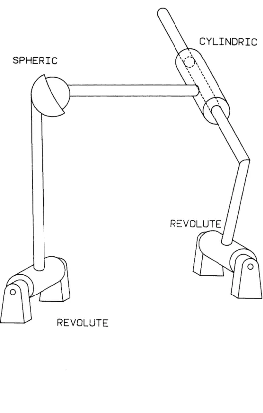
Figure 1. An RSCR Spatial Mechanism ... 4

Figure

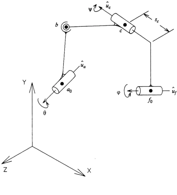
2. Schematic of the RSCR Spatial Mechanism ... 13

Figure

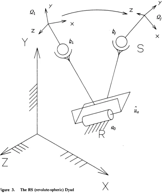
3. The RS (revolute-spheric) Dyad ... 32

Figure

4. The RC (revolute-cylindric) Dyad ... 36

Figure

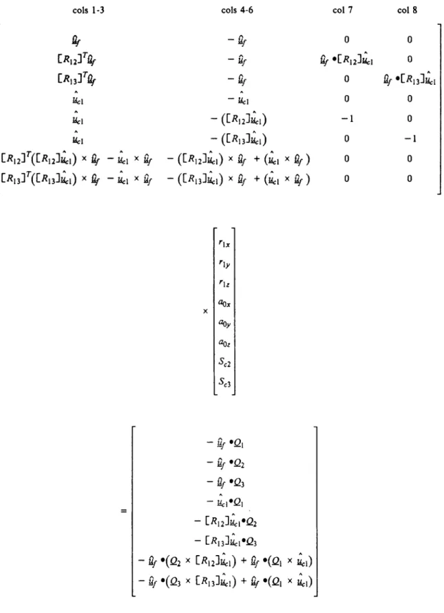
5. RC Dyad Synthesis Equations ... 43

Figure

6. Flowchart of Program RSCR ... 47

Figure

7. Flowchart of Subroutine SYNTH ... 48

Figure 8. Flowchart of Subroutine RSDYAD ... 49

Figure 9. Flowchart of Subroutine RCDY AD ... 50

Figure 10. Flowchart of Subroutine ANALIN ... 52

Figure 11. Flowchart of Subroutine RSC RAN ... 53

Figure 12. Flowchart of Main Program MECHIN ... 56

Figure 13. Flowchart of Subroutine ANIN ... 57

Figure 14. Flowchart of Subroutine WRANAL ... 58

Figure 15. Format of Analysis Data File ... 60

Figure 16. Local Coordinate Systems for a Binary Link ... 63

Figure 17. Position and Attribute Files for a Binary Link ... 64

Figure 18. Position and Attribute Files for an Entire Mechanism ... 65

Figure 19. RSCR Example ... 83

(10)

Chapter 1 INTRODUCTION

There has been a great deal of work done in recent years in the field of computer aided

design and computer aided manufacturing. In particular, efforts in computer aided

manufacturing have stressed the development of robotics. However, there are many

applications where a spatial mechanism could be employed in place of a robot.

Mech-anisms, with no electronic control system, are much less expensive. Closed loop spatial

mechanisms, as compared to robotic manipulators, are capable of carrying greater loads

with less deflection, can run at higher speeds, and have a greater mechanical efficiency.

Single degree of freedom mechanisms are less likely to malfunction than a multi-degree

of freedom, electronically controlled robot. The main drawback to spatial mechanisms

is their specialized nature. A new mechanism must be designed for each new application,

whereas a robot is merely reprogrammed.

(11)

The principle reason spatial mechanisms have not been employed for more applications

is the lack of a unified theory for mechanism design and analysis. The average machine

design engineer is not familiar enough with mechanism design theory to design spatial

mechanisms. Graphical methods, popular in dealing with planar mechanisms, are not

as useful in the design of spatial mechanisms, as at least two projections are required to

completely define the mechanism geometry. Analytical approaches have not been

pop-ular in the past due to the tediousness of calculations involved. However, the increased

availability of the digital computer has spurred the development of spatial mechanism

design theory.

Objectives

This thesis will present design software for the RSCR spatial mechanism. Specifically,

the objectives of this research are to derive in closed form, the displacement, velocity,

and acceleration relationships of the RSCR spatial mechanism using link constraint

equations, to synthesize an RSCR spatial mechanism for rigid body guidance using

dyadic synthesis, and to implement this theory on the computer. Included in this

com-puter implementation are interfaces to existing programs providing for graphical input

of mechanism data, and automatic model generation of a mechanism. Although the

synthesis section of this thesis deals primarily with rigid body guidance, the motion

characteristics presented are also applicable to function generation and path generation.

This thesis is intended to form a part of a computer aided design system for spatial

mechanisms currently being developed in the Mechanical Engineering Department of

(12)

Virginia Polytechnic Institute and State University under the direction of Dr. Arvid

Myklebust and Dr. Charles Reinholtz. Similar design software has been developed for

the RSSR[l], the RCCC[2], and RRSS[3] spatial mechanisms.

A diagram of an RSCR spatial mechanism is shown in Figure

1. Literature Review

Before the early 1950's, most mechanism analysis and synthesis relied heavily on

graph-ical methods. Due to the difficulty in visualizing spatial mechanisms, the emphasis of

this graphical was on planar mechanisms. The long calculations involved often made

analytical methods impractical However, with the development of the digital computer

to handle these calculations, analytical methods began to receive more attention. This

naturally led to the development of analytical theories of spatial mechanism design.

Freudenstein played a major role in the development of modern kinematic theory in the

United States. He led the movement toward analytical methods with his landmark paper

"Approximate Synthesis of Four-Bar Linkages"[4], published

in

1955. In this paper,

Freudenstein established an analytical method for synthesizing a planar four-bar

func-tion generator using precision posifunc-tions. In 1959, Freudenstein and Sandor first brought

attention to the digital computer as a kinematic design tool by publishing the paper

"Synthesis of a Path Generating Mechanism by a Programmed Digital Computer"[5].

(13)

CYLINDRIC

SPHERIC

REVOLUTE

Figure I. An RSCR Spatial Mechanism

(14)

Denavit and Hartenburg[6] developed symbolic notation that has become the rule in

describing the kinematic characteristics of lower pair mechanisms. In 1960, the same

authors extended Freudenstein's work to the synthesis of four-bar spatial mechanisms,

specifically, the RSSR and RCCC spatial mechanisms[?].

A number of German and Russian authors were also active in this period. Beyer[8,9]

used descriptive geometry and vector algebra in spatial mechanism design.

Dimentberg[ 10, 11] developed the powerful screw method for synthesis of lower pair

spatial mechanisms. Other authors include Novodvorskii[12], Stepanov[13], and Levitsk.i

and Shakvazian[14]. English reviews of these works can be found by Beyer[15],

Yang[16], and Harrisberger[17].

For several years, only function generation for spatial mechanisms had been covered in

the literature. However, in 1965 Wilson[18] introduced the problem of rigid body

guid-ance for spatial mechanisms, and demonstrated that function generation could be treated

as a rigid body guidance problem using the principle of inversion. Suh and Radcliffe

developed a method using the 4x4 displacement matrix in the design of planar

linkages[ 19), and spherical linkages[20]. Suh also used the displacement matrix to

syn-thesize spatial mechanisms[21]. These works are based on Suh's doctoral research[22].

Sandor[23] and Sandor and Bisshopp[24] used dual number quarternions and stretch

rotation vectors to develop loop closure equation for spatial mechanisms.

In 1967, Roth studied rigid body motion through finitely separated positions[25], and

applied the results to synthesis of spatial mechanisms[26). Tsai and Roth[27] synthesized

open loop kinematic chains using screw triangle geometry. Kohli and Soni[28] used pair

geometry constraints and successive screw displacements as a basis for synthesizing

spatial mechanisms.

(15)

Some recent work has emphasized the optimization of spatial mechanisms. Perhaps the

most comprehensive work in this area is Reinholtz's doctoral dissertation[29].

Although the appearance of the RSCR spatial mechanism in the literature is rather

scarce, a few authors have used the RSCR as an example, though sometimes the

prob-lem is simplified by using a special configuration of the RSCR. Osman and Segev[30]

employed constant distance equations in analyzing spatial mechanisms. Osman, Bhagat

and Dukk.ipati[31] present a method based on train components. Both of these methods

are iterative, and both are based on the assumption that the axes of the cylindric joint

and second revolute joint are parallel.

Huang and Youm[32] present a method for the displacement analysis of spatial

mech-anisms based on the direction cosine matrix. Their example of the RSCR however, is

another special case, because it is based on the assumption that the axes of the cylindric

joint and second revolute joint intersect.

Funabashi, Ogawa and Hara[33] derive general transformation functions for four-bar

spatial function generators with fixed pivots that are either revolute or prismatic joints.

A general case of the RSCR is presented as an example.

The German authors Gunther, Kassamanjan, and Seyffarth[34] have developed a

graphical method based on projective geometry, and use this method to synthesize the

RSCR for 3 precision positions.

(16)

Chapter 2 ANALYSIS OF THE RSCR SPATIAL

MECHANISM

Rotation Matrices

A rigid body transformation can be defined to be any linear translation and/or rotation

of the body where all points within the body maintain the same relative position. In

other words, the scalar distance between any two points within the body remains the

same regardless of the translation. Any translation of a rigid body can be expressed as

a linear displacement of a reference point fixed in the body, plus an angular rotation of

the body. There are three popular methods of expressing this rotation. The first is a

series of three rotations about a set of Cartesian axes. The second method employs

Euler's angles, and is frequently used in describing the motion of spinning bodies.

(17)

The third method, and the method used in this thesis, consists of a single rotation

q>

about an axis

.U

located arbitrarily in space. This can be best visualized by first rotating

the body about the x and y-axes to bring

u

parallel to the z-axis, rotating the body an

angle

q>

about the z-axis, then reversing the previous rotations to bring

u

back to its

or-iginal position. Using this method, the spatial rotation matrix

[~

.•

J

can be derived.

u;v<p

+

Cq>

+

uxS<i> u;vq>

+

Op

where:

"

versq>

= 1 - cos q>

Using this method, the components of the rotated vector .}!

1

can be determined by

pre-multiplying it by the spatial rotation matrix [Rci.J .

[2.2]

This is one of the most useful forms for describing rotations in kinematics. The spatial

rotation matrix can also be expressed explicitly in q>:

[2.3]

(18)

where:

0

-uz _Uy

[Pu]=

Uz

0

-ux -Uy Ux

0

2 Ux Uxliy UxUz

[Qu]

= UxUy Uy 2 UyUz

2

Uxz UyUz Uz

Note that

where [/]is the 3x3 identity matrix.

The rate of change of position of a vector can be found

by

differentiating Eq. 2.2

[2.4]

From Eq 2.2, and recognizing the rotation matrices to be orthogonal

Therefore

or, since

v

1 =

0

(19)

I

=

[~,uJ[~,uJT.l!

i

=

[W].!!

where [

W]

is the spatial angular velocity matrix.

0

- 'Pz 'Py

0 [W]

=

_'Pz

0

- <px

=

<p Uz - 'Py 'Px

0 -Uy

-uz Uy

0

-ux Ux

0 =~[Pu]

[2.5]

[2.6]

[2.7]

Alternatively, an expression for.!! in terms of

.!!1

can be found. This is is quite simple

if

the axis of rotation is fixed. Differentiating the expanded form of the rotation matrix,

Eq. 2.3,

[2.8]

[2.9]

where:

[2.10]

Hence,

[2.11]

Note that if

Y. is fixed, Eq. 2.6 and Eq. 2.11 are related in that

(20)

Thus,

[2.12]

An expression for the spatial angular acceleration matrix [

W]

is found

by

twice

differ-entiating the rotation matrix [

R.,,J

as

<p

approaches zero.

[2.13]

where

[2.14]

if

.U

is fixed, a simple expression for

.ii

in terms of

J!1

can be found. Differentiating Eq.

2.11 [2.15]

[2.16]

where

[2.17]

[2.18]

(21)

Mechanism Description

A schematic diagram of the RSCR spatial mechanism is shown in Figure 2. Note that

the vectors locating the various points in the global reference frame are not shown on

the figure.

The following notation is used in describing the mechanism in its initial position:

AQ, .fa-vectors defining the fixed location of the two r-evolut• joints.

" "

Ya' Yf-unit vectors defining the fixed axes of rotation of the two revolute joints. bi-vector defining the location of the spheric joint in its initial position. g1-vector defining the location of the cylindric joint in its initial position.

"

.ldcl-unit vector defining the axis of the cylindric joint in its initial position.

As the mechanism is displaced from its initial position, the following symbols are

·de-fined:

0-angle of rotation of input revolute joint about its axis.

b-vector defining the location of the spheric joint in its displaced position. g-vector defining the location of the cylindric joint in its displaced position.

"

ye-unit vector defining the axis of cylindric joint in its displaced position.

~-angle of rotation of input revolute joint about its axis.

Sc-scalar displacement of cylindric joint along its axis.

(22)

"

b

"

y

"

• fo

x

Figure 2. Schematic of the RSCR Spatial Mechanism

(23)

As the mechanism is put in motion, the input (revolute-spheric)

link

rotates about its

axis, and the output (revolute-cylindric) link rotates about its axis. The motion of the

coupler link is more complicated. The coupler link pivots about the moving spheric

joint, and at the same time rotates about and slides along the moving cylindric joint axis.

Hence, the coupler link is subject to Coriolis acceleration, or acceleration relative to a

rotating reference frame.

Displacement Analysis

While based on existing kinematic theory, the remainder of the material presented in this

chapter is original, to the best of the author's knowledge. As the input link of the RSCR

spatial mechanism is displaced from its initial position, there are three unknown

anism parameters that must be determined to describe the displacement of the

mech-anism. These unknowns are the output angle

q>,

and the cylindric joint rotation

'I'

and

displacement

sc.

Two constraint equations are used to determine these unknowns. The

first constraint states that the angle the coupler link makes with the cylindric joint axis

must remain constant through any displacement. This constraint is also known as the

plane equation, and is expressed mathematically in Eq. 2.19

"

(b_ -

-').Ye

=

(121 - -'1).

Yet

[2.19]

or, rearranging

(24)

" " "

12..

Mc

-

.k •

Mc

=

(12.1

-

.k1) •

Met

[2.20]

Note that the location of the displaced spheric joint can easily be found from the input

angle 0.

[2.21]

The displaced cylindric joint location can be expressed as a rotation

q>

about

il,

combined

with a displacement

s.

along

ik.

or,

[2.22]

Substituting the expression for

.k

from Eq.

2.22 for

.k

in Eq.

2.20 and rearranging

"

- (b.1 - .k1).

Met

(R...,~ikl

-

(.QI -

-'1)

e

~I

=

0 [2.24]

Solving for

s.

The second constraint equation for the RSCR mechanism requires that the coupler link

maintain a constant length. Mathematically, this is expressed as the self scalar product.

Substituting from Eq.

2.22 for-'

Expanding Eq.

2.27 Q

• Q

-

2.Q

• [Rcr,u~{-'1

-

J-0) -

2.Q •

Sc[Rcr.u

₁

Jik1

-

2.Q

• J-0

+

[~,u~(-'1

-

J-0) •

[RCl..,~(-'1

-

J-0)

+

2[Rcr,u~(-'1

-

J-0) •

sc[Rcr.u~~I

+

2[Rcr,u/](-'1 -

J-0) • J-0

+

sJRcr.u~ik1

e

sc[Rcr,u~~I

+

2sJR.,,u

₁

1~1

•J-0

+f-0

•J-0

=

(121 - -'1) • (121 - -'1)

Three terms of Eq.

2.28 can be simplified using the following identities:

ANALYSIS OF THE RSCR SPATIAL MECHAl'\/ISM

[2.26]

[2.27]

[2.28]

(26)

[2.28a]

[2.28b]

[2.28c]

With these, Eq. 2.28 becomes

[2.29]

Substituting for

s"

from Eq. 2.25, it can be shown that

[2.30]

where

A

represents those terms that are not a function of the output angle

q>

(27)

A

=

12

•

12 -

212

• J-0

+

(~1

-

J-0) •

(~1

-

J-0)

[2.31]

It is desired to develop an expression explicit in the output angle

<p.

This can be

ac-complished by substituting the expanded form of the spatial rotation matrix from Eq.

2.3 into Eq. 2.30.

The result is an equation of the form

D

cos

2_<p

+

_E

_sin

2_<p

+

_F

_cos

_<p

+

_G

_sin

_<p

+

_H

_cos

_<p

_sin

_<p

+

_K

₌

₀

_[2.32]

where:

(28)

F=

{

+2fl•[P"][P"](~

1 -J(i)}

+2{fl•[P"][P"J~1}{fl•[Q"J~1}

- 2{JO •

[P"][P"]~t}

{fl•

[Q"J~1}

- 2{JO •

[Q"]~

1 }

{fl•

[P"][P"]~t}

+ 2{('1 - JO)•

~

1 }

- 2{JO • [P"][P"](,1 - JO)}

+ 2{('1 - JO)•

~

1 }

{JO•

[P"][PJ~

1 }

+ 2{JO •

[P"][P"J~1}

{JO•

[Q"J~1}

G

=

-2fl

• [P"](,1 - JO) -

2{fl

• [P"J~1}{fl

• [Q"J~1}

+ 2{JO •

[Q"]~t}

{fl•

[P"]~t}

+ 2{('1 - JO)•

~t}

{fl•

[P"]~t}

+ 2{JO •

[P"]~t}

{

b.

• [Q"]~t}

+ 2{JO •

[Pu](,1

-

JO)}

- 2{('1 -

JO)•

~1}

{JO•

[P"]~t}

- 2{JO • [PJik1}

{JO•

[Q"]~t}

H

=

2{

b.

• [P"][P"]~

1 }

{

b.

• [P"]~

1 }

- 2{JO •

[P"][P"]~

1 }

{

b.

• [P"]~

1 }

- 2{JO •

[P"]~

1 }

{

b.

• [P"][P"]~t}

+2{JO •

[P"][P"]~t}

{JO• [Pu1rk1}

(29)

Using the tan half-angle substitution for cos

q>

and sin

q>

I - tan

2(

T)

cos

q> =

I

+

tan

2(

T)

2tan(

T)

sin

q>

=

---1

+

tan

2(

T)

and some manipulation, the result is

(D

-

F

+

K)

tan

4 (

T)

₊

(2G -

2H)

tan

3 (

T)

+ (

-2D

+

4E

+

2K)

tan

2(

T)

+

(2G

+

2H)

tan(

T)

+

(D

+

F

+

K)

=

0 [2.33]

After normalizing, the resultant quartic equation has the form

[2.34]

(30)

the roots of which can be found in closed form. The method used in solving this

equation is discussed in Appendix A. Note that

if

Eq. 2.34 has no real roots for a

par-ticular value of 0, then the mechanism can not assemble in that position.

Once

q>

is known,

s.

and£ can be found from Eq. 2.22 and 2.25 respectively.

The method used in determining the cylindric joint angle

'V

may be somewhat difficult

to visualize. The vector

(b.

-

£) can be found by rotating the vector

(b.

1 -

£

1)

first an

angle

q>

about the axis

.H,,

then an angle

'V

about the axis M_.

That is

[2.35]

Note that the translation

s.

does not enter into this equation, as it does not effect the

orientation of

(b.

- -')·

Defining

Then, from the definition of the scalar product

rearranging

(h1 - £1)'.

(.Q

-

£)

cos"'

=

-I

Ch1 - £1Yl ICh - £)1

Since the length of the coupler link is constant,

ANALYSIS OF THE RSCR SPATIAL MECHANISM

[2.36]

[2.37]

[2.38]

[2.39]

(31)

The sign of

'I'

can be found by crossing [

R

₁₁

,

11

~(lz

1

-

-'i) into

(iz

- -')·

If

the direction of

the result is the same as that of

i,

'I'

is positive.

If

it is in the opposite direction, then

'I'

is negative. The direction of the cross product is found by taking the scalar product

of the cross product and

i.

If

they are the same direction, the scalar product will be

positive, while the scalar product will be negative if they are opposite directions.

"

{(b1 - k})'

x

(Q

-

k)}

·Ye>

0 _0°

< "' <

180°

"

{ (b1 - k} )'

x

(b

-

k)} •

Ye

<

0 - 180°

< "' <

0°

Velocity Analysis

The velocity analysis of the RSCR mechanism is presented in this section.

It

is desired

to find the angular velocity

~

of the second revolute joint, and the angular velocity

\jt

and sliding velocity

s.

of the cylindric joint. The velocity analysis is performed by taking

the time derivative of the displacement constraint equation and then algebraically

ma-nipulating it to get a result explicit in

~

. Once

~

is known,

s.

and

\jt

follow as shown.

The velocity constraint equation is found by taking the derivative of the displacement

constraint equation, Eq. 2.26.

[2.40]

(32)

.

}2

{ (b

-

~.)

_•

_(b

_-

~) =

0 [2.41]

where

b.

is found from

b

= [

W](ll

-

.«o)

=

0 [

V~,u](ll1

-

.«o)

[2.42]

An expression for

~

is found by differentiating Eq. 2.22:

[2.43]

[2.44]

An expression for

sc

is found by differentiating Eq. 2.25:

[2.45]

[2.46]

Substituting Eq. 2.46 into Eq. 2.44, and Eq. 2A4 into Eq. 2.41, and using the

relation-ships:

~

= [

R~.u;J~i

A A

(ll

-

~).Mc =

(ll1 -

~1).

Yet

it can be shown that

(33)

.

x

<p = -

_y

[2.47]

where:

The

quantities~

and

sc

now can be found from Eq. 2.44 and Eq. 2.46 respectively. The

angular velocity of the cylindric joint is found by differentiating Eq. 2.38

Thus,

o/( -

sin 'I')

=

{

~[[

Vq>,uJcl21 - £1)] •

(12

-

£)

+

[Rq>,u_;l(l21

- £1) •

(12

-

£)}

1(121 - £1)1

2

o/

= {

~[[

V<1>,u](l21

-

£1)] •

(b.

-

£)

+

[Rci.u_;l(l21

-

£1) •

(12

-

£)}

( - sin 'I') 1(121 - £1)1

2

[2.48]

[2.49]

[2.50]

(34)

Acceleration Analysis

The angular acceleration,

~

, of the output link is found by differentiating Eq. 2.47:

where:

d

· d

(x)

dt<<p)

=

dt

y

..

1 d

x

d

<p

=--X---Y

_y

_dt

_y2

_dt

d

..

.

-x

= -

12

• (12

- -') -

12

• (12

-

~)

dt

b.

is found from the input acceleration and velocity:

..

d

.

..

. .

12 =

dt

(12)

=

9 [

Ve.J(/2

1 -

~)

+

9 [

V

9

,u](12

1 -

~)

[2.51]

[2.52]

[2.53]

(35)

s.,

Q,

and 'if

are found by differentiating Eq. 2.46, 2.44, and 2.50 respectively

[2.54]

[2.55]

[2.56]

[2.57]

'if

is found by differentiating Eq. 2.50.

(36)

o/

= [

[~.u](/21

- .k1) •

(12

-

.k)

+

2[

~.u](b1

- .k1) •

(k -

D

+

[R<p,u](b1 - .k1) •

(h

-

~)]

I

(b1 - .kt)

I

2

sin o/

(cos

o/)o/

+ .

[2.58]

sm o/

(37)

Chapter 3 SYNTHESIS OF THE RSCR SPATIAL

MECHANISM

While the previous chapter dealt with analysis of a specified mechanism, this chapter

will deal with mechanism synthesis. Mechanism synthesis is the task of designing a

mechanism to perform a specified motion, while analysis is determining the motion of a

specified mechanism. There are usually three steps in synthesizing a mechanism. The

first step is

type

synthesis, determining the type of mechanism to solve a problem.

Pos-sibilities include gears, cams and linkages. The second step in the synthesis process is

number

synthesis: choosing the number of links in the mechanism. There is very little

theory available to the machine design engineer involved in these first two steps,

expe-rience and intuition are the designer's principle tools.

There has been much more work done in the third step of the synthesis problem:

di-mensional

synthesis.

It

is in this step that the necessary link lengths, joint positions and

(38)

orientations are determined. Since this thesis deals strictly with the RSCR spatial

mechanism, only dimensional synthesis will be investigated.

In general, there are three main categories of synthesis problems:

function generation,

path generation,

and

rigid body guidance.

A brief explanation of each category follows.

Function Generation

Function generation deals with coordinating motion of two or more links in the

mech-anism. This usually involves coordinating the angular orientations of the input and

output links. Through the principle of kinematic inversion, function generation may

also be treated as a problem in rigid body guidance.

Path Generation

A path generating mechanism guides a point, called the tracer point, on the mechanism

through a specified path. When the motion of the tracer point is coordinated with the

motion of the input link, it is called path generation

with prescribed input timing.

The

path generation problem may also be treated as an incompletely specified problem in

rigid body guidance.

(39)

Rigid Body Guidance

The third synthesis category involves guiding a rigid body through a specified motion.

This motion is usually specified as a series of finitely separated positions and orientations

of the body. The motion of the body is exact at these

precision

positions, and

approxi-mates the desired motion elsewhere. This thesis presents only synthesis procedures for

rigid body guidance,but since function generation and path generation problems may

be treated as body guidance problems, the techniques presented will have broad

appli-cation.

Dyadic Synthesis

A dyad is a two link kinematic chain, one link connected a known reference frame,

usually ground, and the other connected to the moving body. The dyadic synthesis

ap-proach is so named because the mechanism is designed in dyads; that is, each

con-straining link is determined independently, then assembled to form a closed loop

mechanism. Because of this, dyads are sometimes called the building blocks of

mech-anism synthesis.

Using dyadic synthesis, it is relatively easy to design a mechanism. The first step is to

determine the physical constraints of the dyad, express these physical constraints

math-ematically, write the constraint equations in terms of the unknown joint variables, then

solve the equations for the unknown joint locations and orientations. The theory

(40)

sented in this section is based on the work of Reinholtz[27] However, to provide

conti-nuity, the notation used in this thesis differs somewhat from that found in the source.

RS Dyad Synthesis

A diagram of the RS(revolute-spheric) dyad appears in Figure 3. Note that the vectors

locating the various points in the global reference frame are not shown. The notation

used is similar to that used earlier, and is defined as follows:

•o-fixed location of revolute joint in the global reference fr11111B.

"

y8-unit vector defining the revolute joint axis.

bi-initial location of the spheric joint in the global reference frame.

b;-location of the spheric joint in the j-th position, relative to global reference fra11111. Qi-initial location of moving reference frame (rigid body) relative to global reference frame. Q; -location of moving reference frame in the j-th position, relative to global reference f,...., [R1;J-rotation matrix describing the rotation of local reference frame

from first position to j-th position.

There are three constraint equations with the RS dyad. The first one requires the R-S

link to maintain constant length. This is expressed mathematically using the self-scalar

product.

(41)

y

QI

z

x

z

x

y

_s

Figure 3. The RS (revolute-spheric) Dyad

x

(42)

j=

2,3

[3.1]

The second constraint requires the angle between the R-S

link

and the revolute joint axis

to remain constant. Since kinematically the R-S link will behave the same regardless of

the actual location of the revolute joint on its axis, it can be treated as

if

the R-S link is

perpendicular to the revolute joint axis. This can be expressed mathematically using the

scalar product.

j

=

1,2,3

[3.2]

The final constraint equation requires the spheric joint to be fixed in the moving

refer-ence frame.

j=

2,3

[3.3]

Equations 3.1, 3.2, and 3.3 yield 11 scalar equations in 14 unknowns. The unknowns

are

12.

1,

12.

2,

~

•

.GJ,

and Mo·

Thus, there are three free choices. One option in choosing these

free choices is specifying the initial location of the spheric joint. The spheric locations

12.2

and

12.

3

can then be easily found from Eq. 3.3.

12.2

=

Q2

+

[R12J(12.1 -

Q1)

12.3

=

Q3

+

[R13](12.1 -

Q1)

[3.4]

[3.5]

Thus, this effectively specifies the location of the spheric joint on the rigid body. The

revolute joint axis must be perpendicular to the plane defined by the endpoints of vectors

12.

1,

12.

2, and~

The expression is normalized to yield a unit vector.

(43)

[3.6]

Writing Eq. 3.1 for

j

=

2,3 and combining terms results in

[3.7]

[3.8]

Expanding Eq. 3.2 with

j

=I yields

[3.9]

Equations 3.7, 3.8, and 3.9 represent three linear equations in three unknowns:

-'lox•

.ao,,

.GJ..

This yields, after some manipulation, the following vector equation:

b1x - b1x b1y - b1y b2z - biz lloy b3x - b1x b3y - b1y b3z - biz lloz

[3.10]

which can be easily solved using a method such as Cramer's rule. After solving, the R-S

dyad is completely specified.

(44)

RC Dyad Synthesis

A schematic diagram of the RC dyad appears in Figure 4. Note that the vectors locating

the various points in the global and moving reference frames are not sho\vn on the

fig-ure. The notation used is defined below.

fo

-fixed location of revolute joint relative to global reference frame.

Yf -111it vector vector defining revolute joint axis.

gl -initial location of cylindric joint relative to global reference frame.

gj -location of cylindric joint in j-th position.

Ycl -111it vector defining cylindric joint axis in initial position.

Ycj -111it vector defining cylindric joint axis in j-th position.

sj -scalar displacement of cylindric joint along its axis in j-th position.

rj -location of cylindric joint in j-th position relative to moving coordinate system.

(45)

y

z

x

y

R

Figure 4. The RC (revolute-cylindric) Dyad

x

SYNTHESIS OF THE RSCR SPATIAL MECHANISM

z

c

y

o.

-:J

x

36

(46)

a;

-location of llDVing coordinate syst- in j-th position, relative to global referwioe f,...,

[R1;J -rotation •trix defining rotation of moving coordinate syst- fro11 initial position to j-th position.

Note that the following defining equations hold:

[3.11]

[3.12]

[3.13]

[3.14]

The vector

(k/ -

k)

is constrained to remain perpendicular to both the revolute joint

axis and the cylindric joint axis. This constraint is also known as the plane equation·.

j

=

1,2,3

[3.15]

j

=

1,2,3

[3.16]

The twist angle between the two axes is constant.

j=

2,3

[3.17]

A constant link length equation, Eq. 3.18, can also be written.

j=

2,3

[3.18]

(47)

However, these would not be linear in the components of .{;

_{1, -'l•}

~.

andk . Therefore,

an equivalent linear equation expressing the constant moment

of~

about

Mt

is written.

[3.19]

Thus for three position synthesis, there are 12 unknown parameters:

k.

£11

M,,

i,

S221

S

23•

Equations 3.15, 3.16, 3.17, and 3.19 represent 10 scalar equations in these 12 unknowns,

hence there are 2 free choices. Since the revolute joint axis is defined by a unit vector,

choosing this vector will satisfy the two free choices.

The constant twist equations, Eq. 3.17, can be rewritten for j

=

2,3

Mei

•

lJ.j

=

Y.ct •

lJ.j

[3.20]

[3.21]

substituting the defining equation, Eq. 3.13:

[3.22]

[3.23]

where

[3.24]

(48)

b11 b12

b13

[R13]

=

h21

h22 b23

b31

b32 b33

The following scalar equations can now be written.

a11 a12

a13

"ct.x "1.x "ct.x

{

a11 a12 a13 "cty

}·

_"IY

=

Ucly

• all

a31 a33 Uclz Ulz "ctz b11 b12 b13 Ucl.x "1.x Ucl.x

{

adding Equations 3.28, 3.29, and 3.30 and some manipulation will show that

A similar result can be found using Eq. 3.27:

SYNTHESIS OF THE RSCR SPATIAL MECHANISM

[3.25]

[3.26]

[3.27]

[3.28]

[3.29]

[3.30]

[3.31]

[3.32]

39

(49)

where:

[3.33]

[3.34]

[3.35]

[3.36]

[3.37]

[3.38]

Since

M.

1

is a unit vector

2 2 2

Uclx

+

Ucly

+

Uclz =

l

[3.39]

Equations 3.31, 3.32, and 3.39 can then be solved for

uc1z

_

[(EC-FB) +(DC-FA)+

]-+

uctz -

±

DB

-

EA

-

DB

l

[3.40]

Uc1i

and

uc

1,

are then given

by

( EC

-

FB)

Uclx =

DB

_

EA

Uclz

[3.41]

( DC

-

FA)

Ucly =

EA

-

DB

Uclz

[3.42]

(50)

Note that

ucb

and hence

ucix

and

uc1,

will

have two values. However, this will affect only

the sense of

i

11

and not the direction, which defines the joint axis.

The defining equations, Eq. 3.11-3.14, can be written for each position:

[3.43]

[3.44]

[3.45]

.QI I

=

~I

=

QI

+

lt

[3.46]

[3.47]

[3.48]

Substituting these results into the remaining constraint equations, Eq. 3.15-3.17, yields:

A

JJ1•

{Qt

+

l1 -

fo}

=

0 [3.49]

[3.50]

[3.51]

" Met • {

01 +

lt -

fo}

=

0 [3.52]

[3.53]

[3.54]

(51)

"

= Y.1•

{Qt

+

lt -

.10}

x

Yet

[3.55]

"

= MJ

•{Qt

+

lt -

.10}

x

Met

[3.56]

Expanding these equations using the rules of vector algebra produces a system of eight

equations linear in the eight unknowns

.Qo,

r

1,

S

22,

and

S23 •

Solving this system will

completely specify the dimensions and initial position of the RC dyad.

Additional Design Considerations

Fixed Pivot Location and Link Length Ratio

Those joints of a mechanism that are physically attached to the fixed reference frame

are called fixed pivots. The location of these points are usually defined relative to the

global reference frame. While constraints on the location of the fixed pivots will vary

with each particular problem, they are generally easy to apply. In the case of the RSCR

spatial mechanism, the fixed pivots are the two revolute joints, located by the vectors

.Qo

and

f-0

.

A typical constraint might be:

-5

<

llox

<

5,

-5

<

lloy

<

5,

-5

<

lloz

<

5

(52)

cols 1-3 cols 4-6 col 7 col 8

!lj-

-ar

0 0

[R12JT!lj- - 'JJ.f "

_Yr

•[R12J~1

0

[R13]TYr

-ar

0

A

[R13] ([R13]u.:1) x ~ -

~l

x Yf -

([Ri3J~1)

x

fl1

+

(~1

x

Yr)

0 0

'ly x

-

Hf

•Qi

- fil

•Q2

-

[Ri2J~1)

+

ilr

•(Qi

x

~i)

-

Hf

•(Q3

x

[R13]~i)

+

Yr •(Qi

x

~1)

Figure S. RC Dyad Synthesis Equations

(53)

This would restrict the location of the first revolute joint to a cube, centered at the

ori-gin, with edges 10 units in length.

The link length ratio affects the motion characteristics of the mechanism. Too large a

ratio will cause excessive accelerations and transmission forces, while too small a ratio

will limit link rotatability. As with the fixed pivot location, the link length ratio is also

quite easy to apply. For example, applying the constraint

/long

<

IO

I

short

would limit the ratio of longest to shortest link length to be less than 10.

The Order Condition

It is possible to synthesize a mechanism which guides the rigid body through the

speci-fied precision position, but it does so in the wrong order. The

order

of positions the

body traverses depends on both the

sequence

of positions, and

sense

,

or direction, of

traversal. For example, positions 1,2,3 and 3,2, 1 have the same sequence, but opposite

senses. The sense can changed by simply reversing the direction of input link rotation.

It

should also be noted that there is only one possible sequence for three precision

po-sitions. That is, positions 1,2,3; 2,3,l; and 3,1,2 all have the same sequence, they just

start at different points. This can be corrected by altering the initial position of the input

link. Thus, the order condition poses a major problem only when four or more precision

positions are specified.

(54)

Chapter 4 COMPUTER IMPLEMENTATION OF THE

THEORY

The theory presented in the previous chapters has been implemented on the digital

computer in the form of a FORTRAN77 program. This program has been installed on

an IBM 4341 processing system at Virginia Tech. The program consists of one main

program and several subroutines. An explanation of the main program structure and

some significant subroutines is included in the following sections. A listing of the main

program and all subroutines appears in Appendix

C. As part of this computer

imple-mentation, the program has been interfaced with a graphical preprocessor, and a

postprocessor for automatic model generation. Details of these interfaces are included

in this chapter.

(55)

Program Structure

Program RSCR

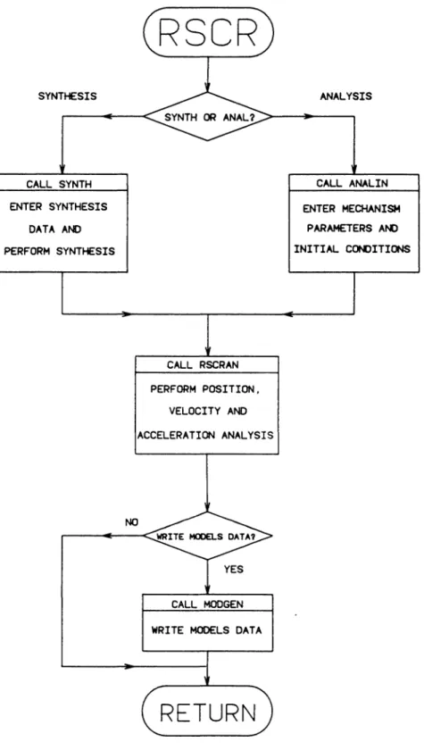
A flowchart of the main program, RSCR appears in Figure 6. This program controls

the overall structure of the entire program. The user has the option of synthesizing a

mechanism, or entering the joint and link data of a known mechanism. In either case,

position, velocity, and acceleration analysis is then performed. After analysis, the user

may choose to create the necessary data files for automatic model generation.

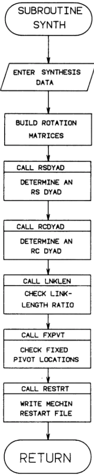
Subroutine SYNTH

A flowchart of subroutine SYNTH appears in Figure 7. This subroutine is called by the

main program to synthesize an RSCR mechanism. This subroutine is used mainly for

data input; actual calculations are performed in the various subroutines called by

SYNTH. The input data consists of three rigid body positions, the vectors and angles

defining the relative orientation of these positions, and the free choice parameters. The

actual format of the data files is given in the next section.

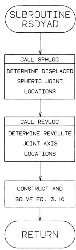
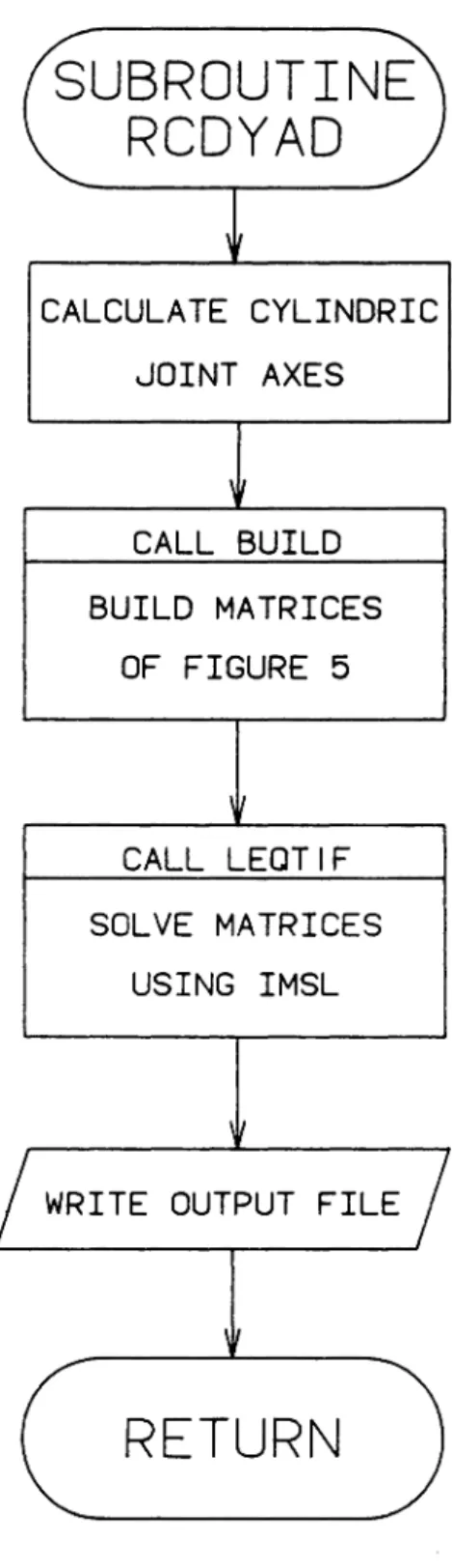
Subroutines RS DYAD and RCDY AD perform the calculations for closed form dyadic

synthesis detailed in Chapter 4. Flow charts of these two subroutines appear in Figures

8 and 9. The link-link length ratio and fixed-pivot locations are checked in subroutines

LNKLEN and FXPVT. A restart file for the graphical preprocessor, as discussed later,

may also be created.

(56)

SYNTHESIS CALL SYNTH ENTER SYNTHESIS DATA AND PERFORM SYNTHESIS

RSCR

CALL RSCRAN PERFORM POSITION, VELOCITY AND ACCELERATION ANALYSIS NO CALL MOOGEN WRITE MODELS DATA

RETURN

Figure 6. Flowchart of Program RSCR

COMPUTER IMPLEMENTATION OF THE THEORY

ANALYSIS CALL ANALIN ENTER MECHANISM PARAMETERS AND INITIAL C()lll)ITIONS

47

(57)

Figure 7. Flowchart of Subroutine SYNTH

SUBROUTINE

SY NTH

ENTER SYNTHESIS DATA BUILD ROTATION MATRICES CALL RSOYAD DETERMINE AN RS DYAD CALL RCDYAD DETERMINE AN RC DYAD CALL LNKLEN CHECK LINK-LENGTH RATIO CALL FXPVT CHECK FIXED PIVOT LOCATIONS CALL RESTRT WRITE MECHIN RESTART FILE

RETURN

(58)

CALL SPHLOC

DETERMINE DISPLACED

SPHERIC JOINT

LOCATIONS

CALL REVLOC

DETERMINE REVOLUTE

JOINT AXIS

LOCATIONS

CONSTRUCT AND

SOL VE EQ . 3 .

I

0 RETURN

Figure 8. Flowchart of Subroutine RSDY AD

(59)

CALCULATE CYLINDRIC

JOINT AXES

CALL BUILD

BUILD MATRICES

OF FIGURE 5

CALL LEQTIF

SOLVE MATRICES

USING IMSL

WRITE OUTPUT FILE

RETURN

Figure 9. Flowchart of Subroutine RCDYAD

(60)

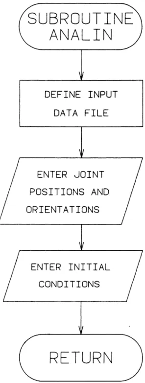
Subroutine ANALIN

A flowchart for subroutine ANALIN appears in Figure 10. This subroutine allows the

user to enter the parameters and initial conditions of a specified mechanism, rather than

synthesizing a mechanism. This subroutine is used strictly for data input; no

calcu-lations are performed.

Subroutine RSCRAN

A flowchart of subroutine RSCRAN appears in Figure 11. This subroutine performs

closed form position, velocity, and acceleration analysis based on the theory in Chapter

3. This analysis is based on default initial conditions if the mechanism synthesized in

SYNTH, or on user specified initial conditions from subroutine ANALIN. The output

of this subroutine consists of 0, 2, or 4 values of each output mechanism parameter at

each input link position, depending on the number of branches of the mechanism. The

output mechanism variables listed are

<p,

tj>,

~.

'I',

o/,

'if,

s.,

and

s.

as defined earlier in

this thesis. An appropriate message is written to the output file if the mechanism does

not assemble at a particular input link position.

(61)

SUBROUTINE

ANAL IN

DEFINE INPUT

DATA FILE

ENTER JOINT

POSITIONS AND

ORIENTATIONS

ENTER INITIAL

CONDITIONS

RETURN

Figure JO. Flowchart of Subroutine A'.'IALI~

(62)

LOOP DESIRED

NUMBER OF

INCREMENTS

Figure 11. Flowchart of Subroutine RSCRAN

COMPUTER IMPLEMENTATION OF THE THEORY

SUBROUTINE

RSCRAN

DETERMINE VECTORS

WHICH DEFINE

INITIAL LINK

LOCATIONS

CALCULATE COEFFICIENTS

OF EQUATION 2.34

AND SOLVE

NO

PERFORM POSITION,

VELOCITY AND

CCELERATION ANALYSIS

WRITE RESULTS TO

OUTPUT FILES

RETURN

53

(63)

Inter/ ace with Graphical Preprocessor

A graphical preprocessor for spatial mechanisms, MECHIN, has been developed in the

Mechanical Engineering Department of Virginia Tech by Thatch[35]. MECH IN allows

the user to define analysis or synthesis problems using interactive computer graphics.

This greatly simplifies the task of problem definition, and drastically decreases the time

required to set up a problem.

MECHIN employs PHIGS(Programmers Hierarchical Interactive Graphics Systems) for

graphics software support, and is graphics device-independent. A wide range of

mech-anism processing code can be supported. The processing codes currently supported are

IMP[36] and RSCR--the code developed for this thesis. As is demonstrated later in this

section, it is relatively easy to modify MECHIN to support additional processing codes.

MECHIN has been designed to permit additional processing codes to be supported with

a minimum of changes to MECH IN. The basic alterations include modification of the

MECH IN menu to allow additional processing code selections, and creation of

subrou-tines to write the data files for the additional processing code. The purpose of this

sec-tion is the briefly explain the MECHIN program structure, and how it can be modified

to support additional processing codes. Though not required, some knowledge of

com-puter graphics may be helpful in understanding the modifications. The reader is referred

to the reference for a more detailed discusssion of MECHIN. All the MECHIN

sub-routines discussed here were written by Thatch as part of the original version of

MECH IN. A listing of selected MECH IN subroutines appears in Appendix D.

COMPUTER IMPLEMENTATION OF THE THEORY 54

I

(64)

The main program MECHIN is very high level. A flowchart appears in Figure 12. The

main program prompts the user to choose between mechanism synthesis or analysis,

then shifts control to the appropriate processor: ANIN for specification of analysis

data, or SYN IN for specification of synthesis data.

A flowchart of subroutine ANIN is shown in Figure 13. The user is queried to either

create a new model , or to modify a previously defined model. Actual model creation

and modification is controlled by subroutine DATA, which is called by ANIN.

ANIN calls subroutine WRANAL to create the data files for the mechanism processing

code. A flowchart of subroutine WRANAL is shown in Figure 14. The user is queried

by WRANAL to choose the appropriate processing code. WRANAL then calls an

ap-propriate subroutine to create a data file for that particular processing code.

The structure is very similar for SYNIN, with subroutines SDA TA and WRSYN taking

the places of DA TA and WRANAL respectively.

An explanation of how MECH IN was modified to support RSCR for mechanism

anal-ysis is presented in the following paragraphs.

The first step in modifying MECH IN to support RSCR was the addition of the choice

RSCR to the processing code choice menu. This was accomplished by slightly modifying

the MECHIN subroutine MENU, which is used to display menu items and process

menu picks. The processing code choices fill the 18th row of array TMENU. :vtany

blank choices have been included in this array to allow for future modifications.

Addi-tional choices may be included by simply replacing a existing blank choice with the new