DynamicMR: A Dynamic Slot Allocation Optimization
Framework for MapReduce Clusters
Shanjiang Tang, Bu-Sung Lee, Bingsheng He
Abstract—MapReduce is a popular computing paradigm for large-scale data processing in cloud computing. However, the slot-based MapReduce system (e.g., Hadoop MRv1) can suffer from poor performance due to its unoptimized resource allocation. To address it, this paper identifies and optimizes the resource allocation from three key aspects. First, due to the pre-configuration of distinct map slots and reduce slots which are not fungible, slots can be severely under-utilized. Because map slots might befully utilized while reduce slots are empty, and vice-versa. We proposes an alternative technique calledDynamic Hadoop Slot Allocationby keeping the slot-based model. It relaxes the slot allocation constraint to allow slots to be reallocated to either map or reduce tasks depending on their needs. Second, the speculative execution can tackle the straggler problem, which has shown to improve the performance for a single job but at the expense of the cluster efficiency. In view of this, we proposeSpeculative Execution Performance Balancingto balance the performance tradeoff between a single job and a batch of jobs. Third, delay scheduling has shown to improve the data locality but at the cost of fairness. Alternatively, we propose a technique calledSlot PreSchedulingthat can improve the data locality but with no impact on fairness. Finally, by combining these techniques together, we form a step-by-step slot allocation system calledDynamicMRthat can improve the performance of MapReduce workloads substantially. The experimental results show that our DynamicMR can improve the performance of Hadoop MRv1 significantly while maintaining the fairness, by up to46% 115%for single jobs and49% 112% for multiple jobs. Moreover, we make a comparison with YARN experimentally, showing that DynamicMR outperforms YARN by about 2%9%for multiple jobs due to its ratio control mechanism of running map/reduce tasks.
Keywords—MapReduce, Hadoop Fair Scheduler, Slot PreScheduling, Delay Scheduler, DynamicMR, Slot Allocation.
!
1
INTRODUCTION
In recent years, MapReduce has become a popular high per-formance computing paradigm for large-scale data processing in clusters and data centers [6]. Hadoop [10], an open source implementation of MapReduce, has been deployed in large clusters containing thousands of machines by companies such as Yahoo! and Facebook to support batch processing for large jobs submitted from multiple users (i.e., MapReduce workloads).
Despite many studies in optimizing MapReduce/Hadoop, there are several key challenges for the utilization and per-formance improvement of a Hadoop cluster.
Firstly, the compute resources (e.g., CPU cores) are ab-stracted into map and reduce slots, which are basic compute units and statically configured by administrator in advance. A MapReduce job execution has two unique features: 1) the slot allocation constraint assumption that map slots can only be allocated to map tasks and reduce slots can only be allocated to reduce tasks, and 2) the general execution constraint that map tasks are executed before reduce tasks. Due to these features, we have two observations: (I). there are significantly different performance and system utilization for a MapReduce workload under different slot configurations, and (II). even under the optimal map/reduce slot configuration, there can be many idle reduce (or map) slots, which adversely affects the system utilization and performance.
S.J. Tang, B.S. Lee, B.S. He are with the School of Computer Engineering, Nanyang Technological University, Singapore.
E-mail:{stang5, ebslee, bshe}@ntu.edu.sg.
Secondly, due to unavoidable run-time contention for pro-cessor, memory, network bandwidth and other resources, there can be straggled map or reduce tasks, causing significant delay of the whole job [2].
Thirdly, data locality maximization is very important for slot utilization efficiency and performance improvement of MapReduce workloads. However, there is often a conflict between fairness and data locality optimization in a shared Hadoop cluster among multiple users [37].
To address the above-mentioned challenges, we present Dy-namicMR, a dynamic slot allocation framework to improve the performance of a MapReduce cluster via optimizing the slot utilization. Specifically, DynamicMR focuses on Hadoop Fair Scheduler (HFS). This is because the cluster utilization and performance for MapReduce jobs under HFS are much poorer (or more serious) than that under FIFO scheduler. But it is worth mentioning that our DynamicMR can be used for FIFO scheduler as well. DynamicMR consists of three optimization techniques, namely,Dynamic Hadoop Slot Allocation (DHSA),
Speculative Execution Performance Balancing (SEPB) and
Slot PreSchedulingfrom different key aspects:
Dynamic Hadoop Slot Allocation (DHSA). In contrast to
YARN which proposes a new resource model of ’container’ that both map and reduce tasks can run on, DHSA keeps the slot-based resource model. The idea for DHSA is to break the assumption of slot allocation constraint to allow that:
(I). Slots are generic and can be used by either map or reduce tasks, although there is a pre-configuration for the number of map and reduce slots. In other words, when there are insufficient map slots, the map tasks will use up all the map slots and then borrow unused reduce slots.
Similarly, reduce tasks can use unallocated map slots if the number of reduce tasks is greater than the number of reduce slots.
(II). Map tasks will prefer to use map slots and likewise reduce tasks prefer to use reduce slots. The benefit is that, the pre-configuration of map and reduce slots per slave node can still work to control the ratio of running map and reduce tasks during runtime, better than YARN which has no control mechanism for the ratio of running map and reduce tasks. The reason is that, without control, it easily occurs that there are too many reduce tasks running for data shuffling, causing the network to be a bottleneck seriously (See Section 3.6).
Speculative Execution Performance Balancing (SEPB).
Speculative execution is an important technique to address the problem of slow-running task’s influence on a single job’s execution time by running a backup task on another machine. However, it comes at the cost of cluster efficiency for the whole jobs due to its resource competition with other running tasks. We propose a dynamic slot allocation technique called
Speculative Execution Performance Balancing (SEPB)for the speculative task. It can balance the performance tradeoff between a single job’s execution time and a batch of jobs’ execution time by determining dynamically when it is time to schedule and allocate slots for speculative tasks.
Slot PreScheduling. Delay scheduling has been shown to
be an effective approach for the data locality improvement in MapReduce [37]. It achieves better data locality by delaying slot assignments in jobs where there are no currently local tasks available. However, it is at the cost of fairness. In view of this, we propose an alternative technique named Slot PreScheduling that can improve the data locality but has no negative impact on fairness. It is achieved at the expense of load balance between slave nodes. By observing that there are often some idle slots which cannot be allocated due to the load balancing constrain during runtime, we can pre-allocate those slots of the node to jobs to maximize the data locality.
We have integrated DynamicMR into Hadoop (particularly Apache Hadoop 1.2.1). We evaluate it using testbed workloads. Experimental results show that, the original Hadoop is very sensitive to the slot configuration, whereas our DynamicMR does not. DynamicMR can improve the utilization and per-formance of MapReduce workloads significantly, with46%
115% performance improvement for single jobs and 49%
112%for multiple jobs. Moreover, we make a comparison with YARN. The experiments show that, DynamicMR consistently outperforms YARN for batch jobs by about2%9%.
The main contributions of this paper are summarized as follows:
Propose a Dynamic Hadoop Slot Allocation (DHSA) technique to maximize the slot utilization for Hadoop.
Propose a Speculative Execution Performance Balancing (SEPB) technique to balance the performance tradeoff between a single job and a batch of jobs.
Propose a PreScheduling technique to improve the data locality at the expense of load balance across nodes, which has no negative influence on fairness.
Develop a system called DynamicMR by combining these
three techniques in Hadoop MRv1.
Perform extensive experiments to validate the effective-ness of DynamicMR and its three step-by-step techniques.
Organization.The rest of the paper is organized as follows.
Section 2 introduces our DynamicMR framework, starting with an overview and then the details on the three techniques, namely, DHSA, SEPB, Slot PreScheduling. Section 3 eval-uates DynamicMR experimentally. Section 4 reviews related work. Finally, Section 5 concludes the paper and gives the future work.
2
OVERVIEW OF
DYNAMICMR
We improve the performance of a MapReduce cluster via optimizing the slot utilization primarily from two perspec-tives. First, we can classify the slots into two types, namely,
busy slots (i.e., with running tasks) and idle slots (i.e., no running tasks). Given the total number of map and reduce slots configured by users, one optimization approach (i.e., macro-level optimization) is to improve the slot utilization by maximizing the number of busy slots and reducing the number of idle slots (Section 2.1). Second, it is worth noting that not every busy slot can be efficiently utilized. Thus, our optimization approach (i.e., micro-level optimization) is to improve the utilization efficiency of busy slots after the macro-level optimization (Section 2.2 and Section 2.3). Particularly, we identify two main affecting factors: (1). Speculative tasks (Detailed in Section 2.2); (2). Data locality (Detailed in Section 2.3). Based on these, we propose DynamicMR, a dynamic utilization optimization framework for MapReduce, to improve the performance of a shared Hadoop cluster under a fair scheduling between users.
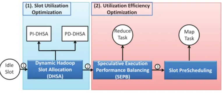
^ƉĞĐƵůĂƚŝǀĞ džĞĐƵƚŝŽŶ WĞƌĨŽƌŵĂŶĐĞĂůĂŶĐŝŶŐ ;^WͿ ^ůŽƚWƌĞ^ĐŚĞĚƵůŝŶŐ LJŶĂŵŝĐ ,ĂĚŽŽƉ ^ůŽƚůůŽĐĂƚŝŽŶ ;,^Ϳ DĂƉ dĂƐŬ ZĞĚƵĐĞ dĂƐŬ WͲ,^ W/Ͳ,^ ;ϭͿ͘^ůŽƚhƚŝůŝnjĂƚŝŽŶ KƉƚŝŵŝnjĂƚŝŽŶ ;ϮͿ͘hƚŝůŝnjĂƚŝŽŶĨĨŝĐŝĞŶĐLJ KƉƚŝŵŝnjĂƚŝŽŶ /ĚůĞ ^ůŽƚ ϭ Ϯ ϯ
Fig. 1:Overview of DynamicMR Framework.
Figure 1 gives an overview of DynamicMR. It consists of three slot allocation techniques, i.e., Dynamic Hadoop Slot Allocation (DHSA), Speculative Execution Performance Balancing (SEPB), andSlot PreScheduling.
Each technique considers the performance improvement from different aspects. DHSA attempts to maximize slot uti-lization while maintaining the fairness, when there are pending tasks (e.g., map tasks or reduce tasks).SEPBidentifies the slot resource in-efficiency problem for a Hadoop cluster, caused by speculative tasks. It works on top of the Hadoop speculative scheduler to balance the performance tradeoff between a single job and a batch of jobs. Slot PreScheduling improves the slot utilization efficiency and performance by improving the data locality for map tasks while keeping the fairness. It pre-schedules tasks when there are pending map tasks with data
on that node, butno allowable idle map slots(See Definition 1 in Section 2.3.1).
By incorporating the three techniques, it enables Dynam-icMR to optimize the utilization and performance of a Hadoop cluster substantially with the following step-by-step processes:
1
. Whenever there is an idle slot available, DynamicMR will first attempt to improve the slot utilization withDHSA. It decides dynamically whether to allocate it or not, subject to the numerous constrains, e.g., fairness, load balance. 2
. If the allocation is true, DynamicMR will further optimize the performance by improving the efficiency of slot utilization with SEPB. Since the speculative execution can improve the performance of a single job but at the expense of cluster efficiency, SEPBacts as an efficiency balancer between a single job and a batch of jobs. It works on top of Hadoop speculative scheduler to deter-mine dynamically whether allocating the idle slot to the pending task or speculative task.
3
. When to allocate the idle slots for pending/speculative map tasks, DynamicMR will be able to further improve the slot utilization efficiency from the data locality opti-mization aspect withSlot PreScheduling.
Moreover, we want to mention that the three techniques are at different levels, i.e., they can be applied together or individually. The detailed description for each technique is given as follows.
2.1 Dynamic Hadoop Slot Allocation (DHSA)
Current design of MapReduce suffers from a under-utilization of the respective slots as the number of map and reduce tasks varies over time, resulting in occasions where the number of slots allocated for map/reduce is smaller than the number of map/reduce tasks. Our dynamic slot allocation policy is based on the observation that at different period of time there may be idle map (or reduce) slots, as the job proceeds from map phase to reduce phase. We can use the unused map slots for those overloaded reduce tasks to improve the performance of the MapReduce workload, and vice versa. For example, at the beginning of MapReduce workload computation, there will be only computing map tasks and no computing reduce tasks, i.e., all the computation workload lies in the map-side. In that case, we can make use of idle reduce slots for running map tasks. That is, we break the implicit assumption for current MapReduce framework that the map tasks can only run on map slots and reduce tasks can only run on reduce slots. Instead, we modify it as follows: both map and reduce tasks can be run on either map or reduce slots.
However, there are two challenges that should be considered as follows:
(C1). Fairnessis an important metric in Hadoop Fair Scheduler
(HFS). We say it is fair when all pools have been allocated with the same amount of resources. In HFS, task slots are first allocated across the pools, and then the slots are allocated to the jobs within the pool [36]. Moreover, a MapReduce job computation consists of two parts: map-phase task computation and reduce-phase task computation. One question is about how to define and ensure fairness under the dynamic slot allocation policy.
(C2). The resource requirements between the map slot and
re-duce slot are generally different. This is because the map task and reduce task often exhibit completely different execution patterns. Reduce task tends to consume much more resources such as memory and network bandwidth. Simply allowing reduce tasks to use map slots requires configuring each map slot to take more resources, which will consequently reduce the effective number of slots on each node, causing resource under-utilized during runtime. Thus, a careful design of dynamic allocation policy is important and needed to be aware of such difference.
With respect to (C1), we propose aDynamic Hadoop Slot Allocation (DHSA). It contains two alternatives, namely, pool-independent DHSA(PI-DHSA) and pool-dependent DHSA (PD-DHSA), each of which considers the fairness from dif-ferent aspects.
2.1.1 Pool-Independent DHSA (PI-DHSA)
DĂƉͲƉŚĂƐĞ WŽŽůϭ DĂƉͲƉŚĂƐĞ WŽŽůϯ ƌĞĚƵĐĞƐůŽƚƐ ŵĂƉƐůŽƚƐ DĂƉWŚĂƐĞ DĂƉͲƉŚĂƐĞ WŽŽůϮ ŵĂƉƐůŽƚƐ ŵĂƉƐů ŽƚƐ ZĞĚƵĐĞͲƉŚĂƐĞ WŽŽůϭ ZĞĚƵĐĞͲƉŚĂƐĞ WŽŽůϯ ZĞĚƵĐĞWŚĂƐĞ ZĞĚƵĐĞͲƉŚĂƐĞ WŽŽůϮ ƌĞĚƵĐĞƐůŽƚƐ ƌĞĚƵĐ ĞƐ ůŽ ƚƐ
Fig. 2: Example of the fairness-based slot allocation flow for PI-DHSA. The black arrow line and dash line show movement of slots between the map-phase pools and the reduce-phase pools.
HFS adopts max-min fairness [17] to allocate slots across pools with minimum guarantees at the map-phase and reduce-phase, respectively. Pool-Independent DHSA (PI-DHSA) ex-tends the HFS by allocating slots from the cluster global level, independent of pools. It considers fairwhen the numbers of typed slots allocated across typed-pools within each phase (i.e., map-phase, reduce-phase) are the same.
As shown in Figure 2, it presents the slot allocation flow for PI-DHSA. It is a typed phase-based dynamic slot allocation policy. The allocation process consists of two parts, as shown in Figure 2:
(1).Intra-phase dynamic slot allocation. Each pool is split into two sub-pools, i.e., map-phase pool and reduce-phase pool. At each phase, each pool will receive its share of slots. An overloaded pool, whose slot demand exceeds its share, can dynamically borrow unused slots from other pools of the same phase. For example, an overloaded map-phase Pool 1 can borrow map slots from map-phase Pool 2 or Pool 3 when Pool 2 or Pool 3 is under-utilized, and vice versa, based on max-min fair policy.
(2). Inter-phase dynamic slot allocation. After the intra-phase dynamic slot allocation for both the map-intra-phase and reduce-phase, we can now perform dynamic slot allocation across typed phases. That is, when there are some unused reduce slots at the reduce phase, and the number of map slots at the map phase is insufficient for map tasks, it will borrow some idle reduce slots for map tasks, to maximize the cluster utilization, and vice versa.
Overall, there are four possible scenarios. LetNM andNR be the total number of map tasks and reduce tasks respectively, whileSM andSRbe the total number of map and reduce slots configured by users respectively. The four scenarios are below: Case 1: When NM ¤ SM and NR ¤ SR, the map tasks are run on map slots and reduce tasks are run on reduce slots, i.e., no borrowing of map and reduce slots.
Case 2: WhenNM ¡SM andNR SR, we satisfy reduce tasks for reduce slots first and then use those idle reduce slots for running map tasks.
Case 3: WhenNM SM andNR¡SR, we can schedule those unused map slots for running reduce tasks.
Case 4: WhenNM ¡SM andNR¡SR, the system should be in completely busy state, and similar to (1), there will be no movement of map and reduce slots.
Thereby, the whole dynamic slot allocation flow is that, Whenever a heartbeat is received from a compute node, we first compute the total demand for map slots and reduce slots for the current MapReduce workload.
Next we determine dynamically the need to borrow map (or reduce) slots for reduce (or map) tasks based on the demand for map and reduce slots, in terms of the above four scenarios. The specific number of map (or reduce) slots to be borrowed is determined based on the number of unused reduce (or map) slots and its map (or reduce) slots required.
In practice, instead of borrowing all unused map (or reduce) slots, we may often want to reserve some unused slots at each phase to minimize the possible starvation of slots for incoming MapReduce jobs. A question would be how to control the number of reserved slots dynamically.
To achieve the reservation functionality, we provide two variables percentageOfBorrowedMapSlots and percentageOf-BorrowedReduceSlots, defined as the percentage of unused map and reduce slots that can be borrowed, respectively. We can thereby limit the number of unused map and reduce slots that should be allocated for map and reduce tasks at each heartbeat of that tasktracker.
With these two parameters, users can flexibly balance the tradeoff between the performance optimization and the star-vation minimization. If users are more prone to performance improvement, they can configure these parameters with large values, as discussed in Appendix F of the supplemental material. On the other hand, if users prefer to avoid starvation, they can set these parameters with small values to reserve some unused slots for incoming tasks, instead of using them immediately.
Moreover, Challenge(C2) reminds us that we cannot treat map and reduce slots the same, and simply borrow unused slots for map and reduce tasks. Instead, we should be aware of varied resource sizes of map and reduce slots. A slot weight-based approach is thus proposed to address the problem. We assign the map and reduce slots with different weight values, in terms of the resource configurations. Based on the weights, we can dynamically determine how much map and reduce tasks should be spawn during runtime. For example, consider a tasktracker with the map/reduce slot configuration of 8/4. According to varied resource requirements, let’s assume that the weights for map and reduce slots are 1 and 2, respectively.
Thus, the total resource weight is81 4216. With slot weight-based approach for dynamic borrowing, the maximum number of running map tasks can be 16 in that compute node, whereas the number of running reduce tasks is at most8{2
48 rather than 16.
Finally, the details of DHSA are shown in Algorithm 1 of the supplemental material.
2.1.2 Pool-Dependent DHSA (PD-DHSA)
DĂƉͲƉŚĂƐĞ WŽŽůϭ ZĞĚƵĐĞͲƉŚĂƐĞ WŽŽůϭ WŽŽůϭ ŵĂƉƐůŽƚƐ ƌĞĚƵĐĞƐůŽƚƐ DĂƉͲƉŚĂƐĞ WŽŽůϮ ZĞĚƵĐĞͲƉŚĂƐĞ WŽŽůϮ WŽŽůϮ ŵĂƉƐůŽƚƐ ƌĞĚƵĐĞƐůŽƚƐ DĂƉͲƉŚĂƐĞ WŽŽůϯ ZĞĚƵĐĞͲƉŚĂƐĞ WŽŽůϯ WŽŽůϯ ŵĂƉƐůŽƚƐ ƌĞĚƵĐĞƐůŽƚƐ ŵĂƉͬƌĞĚƵĐĞƐůŽƚƐ WŽŽůϮ WŽŽů
Fig. 3: Example of the fairness-based slot allocation flow for PD-DHSA. The black arrow line and dash line show the borrow flow for slots across pools.
In contrast to PI-DHSA that considers the fairness in its dynamic slot allocation independent of pools, Pool-Dependent DHSA (PD-DHSA) considers another fairness for the dynamic slot allocation across pools, as shown in Figure 3. It assumes that each pool, consisting of two parts: map-phase pool and reduce-phase pool, is selfish. That is, it always tries to satisfy its own shared map and reduce slots for its own needs at the map-phase and reduce-phase as much as possible before lending them to other pools. It considers fair when total numbers of map and reduce slots allocated across pools are the same with each other. PD-DHSA will be done with the following two processes:
(1). Intra-pool dynamic slot allocation. First, each typed-phase pool will receive its share of typed-slots based on max-min fairness at each phase. There are four possible relationships for each pool regarding its demand (denoted as
mapSlotsDemand,reduceSlotsDemand) and its share (marked as mapShare,reduceShare) between two phases:
Case (a). mapSlotsDemand mapShare, and reduceSlots-Demand ¡ reduceShare. We can borrow some unused map slots for its overloaded reduce tasks from its reduce-phase pool first before yielding to other pools.
Case (b). mapSlotsDemand ¡ mapShare, and reduceSlots-Demand reduceShare. In contrast, we can satisfy some unused reduce slots for its map tasks from its map-phase pool first before giving to other pools.
Case (c). mapSlotsDemand ¤mapShare, and reduceSlots-Demand¤reduceShare. Both map slots and reduce slots are enough for its own use. It can lend some unused map slots and reduce slots to other pools.
Case (d). mapSlotsDemand ¡ mapShare, and reduceSlots-Demand¡reduceShare. Both map slots and reduce slots for a pool are insufficient. It might need to borrow some unused map or reduce slots from other pools through inter-Pool dynamic slot allocation below.
(2).Inter-pool dynamic slot allocation.It is obvious that, (i). for a pool, when itsmapSlotsDemand+reduceSlotsDemand¤
mapShare + reduceShare. The slots are enough for the pool and there is no need to borrow some map or reduce slots from other pools. It is possible for the cases: (a), (b), (c) mentioned above. (ii). On the contrary, whenmapSlotsDemand
+ reduceSlotsDemand ¡ mapShare + reduceShare, the slots are not enough even afterIntra-pool dynamic slot allocation. It will need to borrow some unused map and reduce slots from other pools, i.e., Inter-pool dynamic slot allocation, to maximize its own need if possible. It can occurs for pools in the following cases: (a), (b), (d) above.
The overall slot allocation process for PD-DHSA is as follows:
When a tasktracker receives a heartbeat, instead of allocat-ing map and reduce slots separately, it treats them as a whole during the allocation for pools. It first computes the maximum number of free slots that can be allocated at each round of heartbeat for the tasktracker. Next it starts the slot allocation for pools. For each pool, there are four possible slot allocations as illustrated in Figure 4 below (The number labeled in the graph denotes the corresponding case):
Case (1): We first try the map tasks allocation if there are idle map slots for the tasktracker, and there are pending map tasks for the pool.
Case (2): If the attempt of Case (1) fails since the condition does not hold or it cannot find a map task satisfying the valid data-locality level, we continue to try reduce tasks allocation when there are pending reduce tasks and idle reduce slots.
Case (3): If Case (2) fails due to the required condition does not hold, we try for map task allocation again. Case (1) fails might be that there are no idle map slots available. In contrast, Case (2) fails might be due to no pending reduce tasks. In this case, we can try reduce slots for map tasks of the pool.
Case (4): If Case (3) fails, we try for reduce task allocation again. Case (1) and Case (3) fail might be due to no valid locality-level pending map tasks available, whereas there are idle map slots. In contrast, Case (2) might be that there are no idle reduce slots available. In that case, we can allocate map slots for reduce tasks of the pool.
Moreover, there is a special scenario that needs to be particularly considered. Note it is possible that all the above four possible slot allocation attempts fail for all pools, due to the data locality consideration for map tasks. For example, it is possible that there is a new compute node added to the Hadoop cluster. It may be empty and does not contain any data. Thus, the data locality for all map tasks might not be satisfied and all pending map tasks cannot be issued. The failures of both Case (2) and Case (4) indicate that there are no pending reduce tasks available for all pools. However, there might be some pending map tasks available. Therefore, there is a need to run some map tasks by ignoring the data locality consideration on that new compute node to maximize the system utilization. To implement this, we make a mark visitedForMap for each job visited for map tasks. The data locality will be considered whenvisitedForMapdoes not contain scanned job. Otherwise, it will relax the data locality constrain for map tasks.
Finally, The detailed implementation for PD-DHSA is given in Algorithm 2 of the supplemental material. Moreover, some discussions on DHSA are presented in Appendix C of the
supplemental material. ZĞĚƵĐĞƚĂƐŬ ĂƐƐŝŐŶŵĞŶƚ DĂƉƚĂƐŬ ĂƐƐŝŐŶŵĞŶƚ WĞŶĚŝŶŐŵĂƉ ƚĂƐŬƐĂŶĚŝĚůĞ ŵĂƉƐůŽƚƐ͍ WĞŶĚŝŶŐ ƌĞĚƵĐĞƚĂƐŬƐ ĂŶĚŝĚůĞ ƌĞĚƵĐĞƐůŽƚƐ͍ WĞŶĚŝŶŐŵĂƉ ƚĂƐŬƐĂŶĚŝĚůĞ ƌĞĚƵĐĞƐůŽƚƐ͍ WĞŶĚŝŶŐ ƌĞĚƵĐĞƚĂƐŬƐ ĂŶĚŝĚůĞŵĂƉ ƐůŽƚƐ͍ ;ϰͿ ;ϮͿ ;ϭͿ ;ϯͿ zĞƐ EŽ zĞƐ EŽ zĞƐ zĞƐ EŽ
Fig. 4: The slot allocation flow for each pool under PD-DHSA. The numbers labeled in the graph corresponds to Case (1)-(4) in Section 2.1.2, respectively.
2.2 Speculative Execution Performance Balancing (SEPB)
MapReduce job’s execution time is very sensitive to slow-running tasks (namely straggler) [34]. There are various reasons that cause stragglers, including faulty hardware and software mis-configuration [35]. We classify the stragglers into two types, namely,Hard StragglerandSoft Straggler, defined as follows:
Hard Straggler: A task that goes into a deadlock status
due to the endless waiting for certain resources. It cannot stop and complete unless we kill it.
Soft Straggler: A task that can complete its computation
successfully, but will take much longer time than the common tasks.
For the hard straggler, we should kill it and run another equivalent task, or called abackup task, immediately once it was detected. In contrast, there are two possibilities between the soft straggler and its backup task:
(S1). Soft straggler completes first or the same as its backup
task. For this case, there is no need to run a backup task.
(S2). Soft straggler finishes later than the backup task. We
should kill it and run a backup task immediately. To deal with the straggler problem,speculative executionis used in Hadoop. Instead of diagnosing and fixing straggling tasks, it detects the straggling task dynamically using heuristic algorithms such as LATE [35]. Once detected, however, it can-not simply kill the straggler immediately due to the following facts:
Hadoop does not have a mechanism to distinguish be-tween the hard straggler and the soft straggler;
Moreover, for the soft straggler, it’s also difficult to judge whether it belongs to(S1)or(S2)before running. Simply killing the straggler will harm the case of(S1).
Instead, it spawns a backup task and allows it to run concur-rently with the straggler, i.e., there is a computation overlap between the straggler and the backup task. The task killing operation will occurs when either of the two tasks completed. It is worth mentioning that, although the speculative execution can reduce a single job’s execution time, but it comes at the cost of cluster efficiency [34]. Speculative tasks are not free, i.e., they compete for certain resources, including map slots,
reduce slots and network, with other running tasks of jobs, which could have a negative impact for the performance of a batch of jobs. Therefore, it arises a challenge issue for speculative tasks on how to mitigate its negative impact for the performance of a batch of jobs.
To maximize the performance for a batch of jobs, an intuitive solution is that, given available task slots, we should satisfy pending tasks first before considering speculative tasks. That is, when a node has an idle map slot, we should choose pending map tasks first before looking for speculative map tasks for a batch of jobs. Moreover, recall that in our dynamic scheduler, the map slot is no longer restricted to map task, it can serve reduce task. It means that, for an empty map slot, we should consider choosing tasks in the following order: pending map task, pending reduce task, speculative map task, and speculative reduce task if we want to further maximize the performance for a batch of jobs. We do likewise for reduce slots.
We propose a dynamic task allocation mechanism called
Speculative Execution Performance Balancing (SEPB) for a batch of jobs with speculative execution tasks on top of Hadoop’s current task selection policy. Hadoop chooses a task from a job based on the following priority: first, any failed task is given the highest priority. Second, the pending tasks are considered. For map, tasks with data local to the compute node are chosen first. Finally, Hadoop looks for a straggling task to execute speculatively. In our task scheduling mechanism, we define a variable percentageOfJobsChecked-ForPendingTasks with value domain between 0.0 and 1.0, configurable by users, to control maxNumOfJobsCheckedFor-PendingTasks, which is the maximum number of jobs that are checked for pending map and reduce tasks for a batch of jobs, as shown in Figure 5. Users can balance the tradeoff between the performance for a batch of jobs and a single job’s response time, with speculative task execution. Better performance for the whole job is obtained when percenta-geOfJobsCheckedForPendingTasks is large, Otherwise it will be better for a single job’s response time. The detail of our mechanism is that, when there is an idle map slot, we first check jobs JJ1, J2, J3, ...,K for map tasks. For each job Ji, we compute the total number of pending map and reduce tasks by scanning all jobs between Ji and Jj, where i
1,2,3, ..., ji maxNumOfJobsCheckedForPendingTasks1.
Next, we check each job Ji for the following conditions: (1). No failed map tasks and pending map tasks for job Ji; (2). The total number of pending map tasks is larger than zero;
(3). The total number of pending reduce tasks is larger than zero, andpercentageOfBorrowedMapSlotsis larger than zero. The job Ji will be skipped for looking for speculative map tasks when either Conditions (1) and (2), or Condition (1) and (3) is satisfied. Otherwise, we will scan it for possible specula-tive map tasks, with Hadoop’s speculaspecula-tive task mechanism[34], or LATE [35].
However, delaying the scheduling of speculative task will bring another challenging problem. For the hard straggler or the soft straggler of (S2) that occupies a slot for a really long time, if we do not solve it as early as possible, then
the resource allocated to the slot are being used inefficiently, hence reducing the efficiency of the cluster.
To address this problem, we currently use a simple heuristic algorithm: We estimate the execution time for each task. When it took twice longer than the average execution time of tasks, we kill it directly to yield the slot. Since failed/killed tasks have the highest priority to run in Hadoop, a backup task will be created to replace it quickly, improving the performance of a single job and mitigating the negative impact on the cluster efficiency.
Finally, speculative reduce tasks are handled similarly. The detailed implementation of SEPB is given in Algorithm 3 of the supplemental material.
:ϰ :ϯ :Ϯ :ϭ
:ϱ :ϲ
ŵĂdžEƵŵKĨ:ŽďƐŚĞĐŬĞĚ&ŽƌWĞŶĚŝŶŐdĂƐŬƐ
Fig. 5:The computation policy for thetotalNumOfPendingMapTasks
andtotalNumOfPendingReduceTasks.
2.2.1 Discussion on SEPB VS LATE
The benefit of SEPB over LATE lies in its policy for slot allocation to speculative tasks. For LATE, whenever there is a straggled task for a job, it will create a backup task and allocate a slot to run it immediately from an individual job’s view if the total number of speculative tasks is less than the thresholdSpeculativeCap, a parameter for capping the number of running speculative tasks. In contrast, SEPB performs the resource allocation for speculative tasks from a global view by considering multiple jobs (determined by the argument
maxNumOfJobsCheckedForPendingTasks). It will delay the slot allocation to speculative tasks whenever there are pending tasks for the multiple jobs. Consider an example with 6 jobs as shown in Figure 5. The maxNumOfJobsCheckedForPend-ingTasks is 4 andSpeculativeCap for LATE is 4. Assume at a moment that total number of idle slots is 4, the numbers of straggled tasks for J1, J2, J3, J4, J5, J6 are 5,4,3,2,1,0, nd the numbers of pending tasks forJ1, J2, J3, J4, J5, J6 are
0,0,10,10,15,20, respectively. With LATE, it will spawn 4 speculative tasks forJ1to possess all idle slots. However, with SEPB, it will allocate all 4 idle slots to the pending tasks of J3, J4 to improve the slot utilization efficiency, instead of speculative tasks of J1. The relationship between SEPB and LATE is that, SEPB works on top of LATE and is an enhancement of LATE in scheduling speculative tasks. When LATE detects a straggled task and an idle slot, it first checks the number of running speculative tasks. When it is smaller thanSpeculativeCap, instead of creating speculative tasks for straggled tasks immediately, LATE will inform SEPB. The SEPB then determines whether to create a speculative task to re-compute data or not from a global view by checking multiple jobs. If SEPB finds pending tasks, it will allocate the idle slot to a pending task. If not, a new speculative task will then be created to possess the idle slot.
2.3 Slot PreScheduling
Keeping the task computation at the computing node with the local data (i.e., Data locality) is an efficient and important approach to improve the efficiency of slot utilization and per-formance.Delay Scheduler has been proposed to improve the data locality in MapReduce by [37]. It delays the scheduling for a job by a small amount of time, when it detects there are
no local map tasks from that job on a node where its input data reside. However, it is at the expense of fairness. There is a tradeoff between the data locality and fairness optimization with delay scheduler. It means that, in HFS, delay scheduling is not enough and there is still optimization space for data locality improvement. A challenging question will be: Are there any solutions that can further improve the data locality while have no impact on fairness?
To answer this question, we propose a Slot PreScheduling
technique that can improve the data locality while having no negative impact on the fairness of MapReduce jobs. In contrast to delay scheduler, it is achieved at the expense of load balance across slave nodes. The basic idea is that, in light of the fact that there are often some idle slots which cannot be allocated due to the load balancing constrain during runtime, we can pre-allocate those slots of the node to jobs to maximize the data locality.
2.3.1 Preliminary
In Hadoop task scheduling, there is a load manager that at-tempts to balance the workload across slave nodes, making the ratios of used resources close to each other among slave nodes (i.e., load balancing). Prior to presenting Slot PreScheduling, we start with two definitions:
Definition 1. Theallowable idle map (or reduce) slotsrefer
to the maximum number of idle map (or reduce) slots that can be allocated for a tasktracker, considering the load balancing between machines.
Definition 2. The extra idle map (or reduce) slots refer to
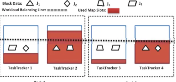
the remaining idle map (or reduce) slots by subtracting the maximum value of used map (or reduce) slots and allowable idle map (or reduce) slots from the total number of map slots for a tasktracker, considering the load balancing between machines. :ϰ :ϭ :Ϯ :ϯ ZĂĐŬϮ dĂƐŬdƌĂĐŬĞƌϰ dĂƐŬdƌĂĐŬĞƌϯ ZĂĐŬϭ dĂƐŬdƌĂĐŬĞƌϭ dĂƐŬdƌĂĐŬĞƌϮ ůŽĐŬĂƚĂ͗ tŽƌŬůŽĂĚĂůĂŶĐŝŶŐ>ŝŶĞ͗ hƐĞĚ DĂƉ^ůŽƚƐ͗
Fig. 6: An example of unbalanced workload distribution of running map tasks in a Hadoop cluster. We assume the current priority order of fair-share allocation is J1ÑJ2ÑJ3ÑJ4.
As illustrated in Figure 6, the workload balancing line shows the current number of map slots that can be used under an ideally balanced case. The allowable idle map slots are illustrated by the white area below the workload balancing
line. We can note that Tasktracker 1 and 3 have some allowable idle map slots, whereas there are noallowable idle map slots
available for Tasktracker 2 and 4. In contrast, all tasktrackers have extra idle map slots (See Definition 2), which are illustrated with the white area above the workload balancing line.
There is a tradeoff between data locality and load balancing. It occurs that, when a job has a local data on a slave node (e.g.,
J1 in TaskTracker 2). The slave node has some idle slots but
the load manager do not allow it to use (i.e., no allowable idle slots) considering the load balancing issue. Improving the data locality in this scenario will hurt the load balancing. Reversely, achieving load balance will negative affect data locality.
2.3.2 Observation and Optimization
In practice, for a MapReduce cluster, the computing workloads of running map (or reduce) tasks between tasktrackers (i.e., machines) are generally varied, because of the following facts.
(1). Lots of MapReduce clusters in real world consist of
heterogeneousmachines (i.e., different computing powers between machines),
(2). There are often varied computing loads (i.e., execution time) for map and reduce tasks from different jobs, due to the varied input data sizes as well as applications,
(3). Even for a single job under the homogenous environment, the execution time for map (or reduce) tasks may still not be the same, due to the skew caused by an uneven distribution of input data to tasks and some portions of the input data might take longer time to process than others [16],
For example, Figure 6 illustrates an unbalanced workload distribution of running map tasks in a Hadoop cluster, con-sisting of two racks each with two machines. To balance the workload, Hadoop provides a mechanism to dynamically control the number of allowable idle map (or reduce) slots
(See Definition 1) for a tasktracker in a heartbeat as the
following three steps.
Step 1#:Compute the load factormapSlotsLoadFactoras the
sum of pending map tasks and running map tasks from all jobs divided by the cluster map slot capacity.
Step 2#: Compute the current maximum number of usable
map slots by multiplying min{mapSlotsLoadFactor,1} with the number of map slots in a tasktracker.
Step 3#: Finally, we can compute the currentallowable idle
map (or reduce) slots for a tasktracker, by subtracting the current number of used map (or reduce) slots from the current maximum number of usable map slots.
Let’s suppose that there are four running jobs and two replicas for each block data in Figure 6. Let’s assume the priority order of fairness allocation is J1 ÑJ2 ÑJ3 ÑJ4. Under the current load distribution, we can see that there are no allowable idle map slots for all those tasktrackers (e.g., Tasktracker 2 and 4) with local block data ofJ1. It means that, based on the delay scheduling,J1will be delayed to schedule within a time limit, at the expense of fairness, no matter which tasktracker connects to the jobTracker in a heartbeat (See more explanations on it in Appendix D of the supplemental material). However, we can see that there are idle map slots
for each tasktracker. If we relax the strict load balancing constrain when Tasktracker 2 or 4 connects to the Jobtracker, we can proactively allocate the extra idle map slots to J1, satisfying both the data locality and fairness requirements. Based on this observation, we propose a scheduler named Slot PreSchedulingto proactively allocate slots to those jobs with local map tasks, aiming to achieve both the data locality maximization and fairness requirement.
There are two cases for using Slot PreScheduling. The first case considers a tasktracker tts on which there are extra idle map slots available, but no allowable idle map slots. For a headed job following the fair-share priority order, when it has local map tasks with block data on thetts, instead of skipping it by the default Hadoop scheduler, we can proactively allocate extra map slots to the job.
The second case is for DHSA. When there are no idle map slots but some idle reduce slots available, for a connected tasktracker tts in a heartbeat, we can proactively borrow idle reduce slots for local pending map tasks and restore them later, in order to maximize the data locality.
2.3.3 Comparison with Delay Scheduler
In this section, we make a comparison and discussion between Delay Scheduler and Slot PreScheduling. First, they consider completely opposite scenarios. That is, Slot PreScheduling works for the case when there are pending map tasks for the current job with local block data on the tasktrackertts, whereas Delay Scheduler considers the case without local pending map tasks. Based on this fact, in our work, we combine them together to improve the data locality. For example, in Figure 6, when the current connected tasktracker in a heartbeat is Tasktracker 1 or 3, the Delay Schedulerwill work to delay the scheduling ofJ1, to improve the data locality. In contrast, when either Tasktracker 2 or 4 connects to the jobTracker, the Slot PreScheduling will work by allocating the extra idle map slots toJ1, improving the data locality and guaranteeing fairness.
Table 1 lists the benefits and costs for Slot PreScheduling and Delay Scheduler under different metrics, including Fair-ness, Data Locality and Load Balance. We can see that, the Slot PreScheduling can benefits (or improves) both fairness and data locality metrics, but at the expense of load balance, since it uses the extra idle map slots. However, for Delay Scheduler, it is favorable for data locality and load balance, whereas at the cost of fairness.
Fairness Data Locality Load Balance
Slot PreScheduling
Delay Scheduler
TABLE 1: Benefit and Cost Comparison between Slot PreSchedul-ing and Delay Scheduler. ’ ’ denotes the benefit, while ’’ repre-sents the cost (or expense).
2.4 Discussion
The goal of our work is to improve the performance for MapReduce workloads while maintaining the fairness across pools when HFS is adopted. To achieve it, we propose a framework called DynamicMR (See Appendix B of the supple-mental material for details on how to implement DynamicMR
into Hadoop system.) consisting of three different dynamic slot allocation policies, i.e., DHSA, SEPB, Slot PreScheduling.
Table 2 summarizes the comparison results for the three policies with respect to different metrics (e.g., fairness, slot utilization, and performance). First, all the three polices are favorable for the performance improvement of MapReduce workloads, due to the benefits from slot utilization optimiza-tion. Specifically, DHSA improves the performance by increas-ing the slot utilization. In contrast, rather than attemptincreas-ing to improve the slot utilization, SEPB and Slot PreScheduling achieve the performance improvement by maximizing the efficiency of slot utilization, under a given slot utilization. For fairness metric, both DHSA and DS (i.e., Delay Scheduler) have an impact on it, whereas SEPB does not. Specifically, PI-DHSA, PD-DHSA and SPS (i.e., Slot PreScheduling) can benefit fair sharing, whereas DS has a negative impact on fairness.
Techniques Fairness Slots Utilization Performance
DHSA PI-DHSA
PD-DHSA
SEPB %F G
DS %F G
SPS
TABLE 2: Benefit and cost comparison for allocation techniques regarding each metric. ’DS’ is an abbreviation for Delay Scheduler, while ’SPS’ is short for Slot PreScheduling. ’ ’ denotes thebenefit. ’’ represents thecost(orexpense). ’%’ denotes theefficiency.
3
EXPERIMENTAL
EVALUATION
In this section, we experimentally evaluate the performance benefit of DynamicMR. We first evaluate the individual im-pact of each optimization technique of DynamicMR (i.e., DHSA, SEPB, Slot PreScheduling in Section 3.2, 3.3 and 3.4, separately). Next, we present the combined performance im-provement achieved by DynamicMR in Section 3.5. Later we compare our DynamicMR with YARN in performance.
3.1 Experimental Setup
We ran our experiments in a cluster consisting of 10 compute nodes, each with two Intel X5675 CPUs (4 CPU cores per CPU with 3.07 GHz), 24GB memory and 56GB hard disks. We configure one node as master and namenode, and the other 9 nodes as slaves and datanodes. The latest version of Hadoop 1.2.1 is chosen in our experiment. We generate our testbed workloads by choosing 9 benchmarks arbitrarily from Purdue MapReduce Benchmarks Suite [1] and using their provided datasets as show in Table 3, where the input data sizes are chosen according to the processing capability of our cluster.
3.2 Performance Evaluation for DHSA
In this section, we first show the dynamic tasks execution processes for PI-DHSA and PD-DHSA. Then we evaluate and compare the performance improvement by PI-DHSA and PD-DHSA under different slot configuration. Third, we make a discussion on the performance influence of the arguments of the percentage of map and reduce slots that can be borrowed for our DHSA in Appendix F of the supplemental material.
Benchmark Input Data
Name Description Data Source Data Size (GB)
WordCount computes the occurrence frequency of each word in a document. wikipedia [29] 10
Sort sorts the data in the input files in a dictionary order. wikipedia [29] 20
Grep finds the matches of a regex in the input files. wikipedia [29] 30
InvertedIndex takes a list of documents as input and generates word-to-document indexing. wikipedia [29] 40 Classification classifies the input into one of k pre-determined clusters. movie ratings
dataset [29] 20
HistogramMovies generates a histogram of input data and is a generic tool used in many data analyses. movie ratingsdataset [29] 20 HistogramRatings generates a histogram of the ratings as opposed to that of the movies based on their
average ratings.
movie ratings
dataset [29] 20
SequenceCount generates a count of all unique sets of three consecutive words per document in the input data.
wikipedia [29]
30 SelfJoin generates association among k+1 fields given the set of k-field associations. synthetic data [29] 40
TABLE 3:The job information for Purdue MapReduce benchmarks and data sets.
Ϭ ϮϬ ϰϬ ϲϬ ϴϬ ϭϬϬ ϭϮϬ ϭ ϯ ϱ ϳ ϵ ϭϭ ϭϯ ϭϱ ϭϳ ϭϵ Ϯϭ Ϯϯ Ϯϱ Ϯϳ Ϯϵ ϯϭ η ŽĨZƵŶŶŝŶŐ dĂ ƐŬƐ dŝŵĞ^ƚĞƉƐ WŽŽůϭͺŵĂƉdĂƐŬƐ WŽŽůϭͺƌĞĚƵĐĞdĂƐŬƐ WŽŽůϮͺŵĂƉdĂƐŬƐ WŽŽůϮͺƌĞĚƵĐĞdĂƐŬƐ WŽŽůϯͺŵĂƉdĂƐŬƐ WŽŽůϯͺƌĞĚƵĐĞdĂƐŬƐ (a) PI-DHSA Ϭ ϮϬ ϰϬ ϲϬ ϴϬ ϭϬϬ ϭϮϬ ϭ ϯ ϱ ϳ ϵ ϭϭ ϭϯ ϭϱ ϭϳ ϭϵ Ϯϭ Ϯϯ Ϯϱ Ϯϳ Ϯϵ ϯϭ η ŽĨZƵŶ ŶŝŶŐ dĂ ƐŬƐ dŝŵĞ^ƚĞƉƐ WŽŽůϭͺŵĂƉdĂƐŬƐ WŽŽůϭͺƌĞĚƵĐĞdĂƐŬƐ WŽŽůϮͺŵĂƉdĂƐŬƐ WŽŽůϮͺƌĞĚƵĐĞdĂƐŬƐ WŽŽůϯͺŵĂƉdĂƐŬƐ WŽŽůϯͺƌĞĚƵĐĞdĂƐŬƐ (b) PD-DHSA
Fig. 7:The execution flow for the two DHSAs. There are three pools, with one running job each.
3.2.1 Dynamic Tasks Execution Processes for PI-DHSA and PD-DHSA
To show different levels of fairness for the dynamic tasks allocation algorithms, PI-DHSA and PD-DHSA, we perform an experiment by considering three pools, each with one job submitted. Figure 7 shows the execution flow for the two DHSAs, with 10 sec per time step. The number of running map and reduce tasks for each pool at each time step is recorded. For PI-DHSA, as illustrated in Figure 7(a), we can see that, at the beginning, there are only map tasks, with all slots used by map tasks under PI-DHSA. Each pool shares 13 of the total slots (i.e., 36 slots out of 108 slots), until the5thtime step. The map slot demand for Pool 1 begins to shrink and the unused map slots of its share are yielded to Pool 2 and Pool 3 from the 6th time step. Next from6th to10th time step, the map tasks from Pool 2 and Pool 3 equally share all map slots and the reduce tasks from Pool 1 possess all reduce slots, based on the typed-phase level fairness policy of PI-DHSA(i.e., intra-phase dynamic slot allocation). From 11thto 18th time step, there are some unused map slots from Pool 2 and they are possessed by map tasks from Pool 3 (i.e., intra-phase dynamic slot allocation). Later, there are some unused map slots from Pool 3 and they are used by reduce tasks from Pool 1 and Pool 2 from 22st to25th time step (i.e., inter-phase dynamic slot allocation).
For PD-DHSA, similar to PI-DHSA at the beginning, each pool obtains 13 of the total slots from the1thto5rdtime step, as shown in Figure 7(b). Some unused map slots from Pool 1 are yielded to Pool 2 and Pool 3 from6thto the7thtime step. However, from the8thto12th, the map tasks from Pool 2 and Pool 3 and the reduce tasks from Pool 1 takes 13 of the total slots, subject to the pool-level fairness policy of PD-DHSA
(i.e., intra-pool dynamic slot allocation). Finally, the unused slots from Pool 1 begins to yield to Pool 2 and Pool 3 since
13thtime step (i.e., inter-pool dynamic slot allocation). 3.2.2 Performance Improvement Comparison
Ϭ Ϭ͘ϱ ϭ ϭ͘ϱ Ϯ Ϯ͘ϱ ϯ ϯ͘ϱ ϰ ϰ͘ϱ ϭͬϭϭ ϮͬϭϬ ϯͬϵ ϰͬϴ ϱͬϳ ϲͬϲ ϳͬϱ ϴͬϰ ϵͬϯ ϭϬͬϮ ϭϭͬϭ ^ƉĞĞĚƵ Ɖ DĂƉƐůŽƚƐͬZĞĚƵĐĞ^ůŽƚƐƉĞƌdĂƐŬdƌĂĐŬĞƌ KƌŝŐŝŶĂů,ĂĚŽŽƉ W/Ͳ,^ WͲ,^
Fig. 8:The performance improvement by DHSA under various slot configuration forSortbenchmark.
Figure 8 presents the performance improvement results in comparison with original Hadoop under various slot con-figurations, for our proposed DHSA (See Figure 2 in the supplemental material for more results of other benchmarks). Note that there are 12 CPU cores per slave node and we assume that one MapReduce slot corresponds to a CPU core. Thereby, we vary the number of map slots per slave node from 1 to 11. Particularly, we define the speeduphere as the ratio of the execution time of the original Hadoop under 1/11 map/reduce slot configuration per slave node, to the current execution time.
We have the following three observations.
Firstly, the original Hadoop is very sensitive to the map/reduce slot configuration, whereas there is little impact for the map/reduce slot configuration on our DHSA (i.e., the speedup keeps stable under different map/reduce slot configurations). For example, there are about1.8x performance differences for Sort benchmark in Figure 8 between the optimal and worst-case map/reduce slot configurations for the original Hadoop.
To explain the reason behind it, let’s take a single job for example. Let NM and NR denote the number of map tasks and reduce tasks. Let tM andtR denote the execution time for a single map task and reduce task. LetSM and SR denote the number of map slots and reduce slots. Moreover, we assume that there is one slot per CPU core and thus
the sum of map slots and reduce slots is fixed for a given cluster. Then for the traditional Hadoop cluster, the execution time will be HNMSMI tM HNRSRI tR. In contrast, it will be
H NM
SM SRI tM HSMNRSRI tR for our DHSA. Based on the formula, we can see varied performance from the traditional Hadoop under different slot configurations. However, there is little impact on the performance for different slot configura-tions under DHSA.
Secondly, compared with the original Hadoop, both PI-DHSA and PD-PI-DHSA can improve the performance of MapReduce jobs significantly, especially under the worst-case map/reduce slot configuration. For example, there are about
2x performance improvement for Sort benchmnark under the worst-case configuration (e.g., the x-axis point 1/11 in Figure 8), with our proposed DHSA.
Thirdly, the performance improvement is stable and very close to each other for both PI-DHSA and PD-DHSA. The reason is that, although PI-DHSA and PD-DHSA have differ-ent fairness concepts (See Section 2.1), they follow strictly the same principle of slot utilization maximization, by switching the allocation of the map/reduce slots for map/reduce tasks dynamically.
3.3 Speculative Execution Control for Performance
Ϭ͘ϵϴ ϭ ϭ͘ϬϮ ϭ͘Ϭϰ ϭ͘Ϭϲ ϭ͘Ϭϴ ϭ͘ϭ ϭ͘ϭϮ Ϭ ϮϬ ϰϬ ϲϬ ϴϬ ϭϬϬ ^Ɖ ĞĞĚƵƉ ƉĞƌĐĞŶƚĂŐĞKĨ:ŽďƐŚĞĐŬĞĚ&ŽƌWĞŶĚŝŶŐdĂƐŬƐ;йͿ ϱũŽďƐ ϭϬũŽďƐ ϮϬũŽďƐ
(a) The performance improvement un-der different percentages.
ϮϬϬ ϯϬϬ ϰϬϬ ϱϬϬ ϲϬϬ ϳϬϬ ϴϬϬ ϵϬϬ ϭ Ϯ ϯ ϰ ϱ dž ĞĐƵƚŝŽŶ ƚŝŵĞ ;ƐĞ ĐͿ :Žď/Ě ƉĞƌĐĞŶƚĂŐĞKĨ:ŽďƐŚĞĐŬĞĚ&ŽƌWĞŶĚŝŶŐdĂƐŬƐсϬй ƉĞƌĐĞŶƚĂŐĞKĨ:ŽďƐŚĞĐŬĞĚ&ŽƌWĞŶĚŝŶŐdĂƐŬƐсϭϬϬй
(b) The detailed job execution time for the workload of 5 jobs.
Fig. 9:The performance results with SEPB.
Recall in Section 2.2, we stated that speculative task execution can overcome the problem of straggler (i.e., the slow-running task) for a job, but it is at the cost of cluster utilization. We define a user’s configurable variable percent-ageOfJobsCheckedForPendingTasks to determine the time to schedule speculative tasks. To validate the effectiveness of our dynamic speculative execution control policy, we perform an experiment with 5 jobs, 10 jobs and 20 jobs by varying the values of percentageOfJobsCheckedForPendingTasks.
Note that LATE [35] has been implemented in Hadoop 1.2.1. Figure 9 presents the performance results with SEPB in comparison to LATE. All speedups are computed with respect to the case that percentageOfJobsCheckedForPendingTasksis equal to zero. We have the following findings:
First, SEPB can improve the performance of Hadoop from
3% 10%, shown in Figure 9(a). As the value of per-centageOfJobsCheckedForPendingTasksincreases, the trend of performance improvement tends to be large and the optimal configurations could be distinct for different workloads. For example, the optimal configuration for 5 jobs is80%, but for 10 jobs is100%. The reason is that, large value of percentage-OfJobsCheckedForPendingTaskswill let more numbers of jobs
be checked for pending tasks before considering speculative execution for each slot allocation, i.e., It is more likely to allocate a slot to a pending task first, rather than a specula-tive task, which benefits more for the whole jobs. However, large value ofpercentageOfJobsCheckedForPendingTaskswill delay the speculative execution for straggled jobs, hurting their performance. For some workloads, too large value of
percentageOfJobsCheckedForPendingTasks will degrade the performance for straggled jobs a lot and in turn affect the overall jobs, explaining why the optimal configuration is not always 100%. We recommend users to configure percenta-geOfJobsCheckedForPendingTasks at 60% 100% for their workloads.
Second, there is a performance tradeoff between an individ-ual jobs and the whole jobs with SEPB. We show a case for the workload of 5 jobs when setting percentageOfJobsChecked-ForPendingTasks to be 0 and 100%, respectively. As results shown in Figure 9(b), Job 2 and 4 are negative affected due to the constrain on speculative execution from SEPB, whereas it favors the performance for whole jobs (i.e., the maximum execution time of jobs).
3.4 Data Locality Improvement Evaluation for Slot PreScheduling ϴϭ͘Ϯϱй ϳϭ͘ϴϴй ϴϱ͘ϲϯй ϵϯ͘ϳϱй ϵϬ͘ϲϯй ϵϳ͘ϱϬй Ϭй ϭϬй ϮϬй ϯϬй ϰϬй ϱϬй ϲϬй ϳϬй ϴϬй ϵϬй ϭϬϬй WĞ ƌĐ Ğ Ŷ ƚ >Ž ĐĂ ůD ĂƉ d ĂƐ ŬƐ tŝƚŚŽƵƚ^ůŽƚWƌĞ^ĐŚĞĚƵůŝŶŐ tŝƚŚ^ůŽƚWƌĞ^ĐŚĞĚƵůŝŶŐ ϭϲŵĂƉƐ ϯϮŵĂƉƐ ϭϲϬŵĂƉƐ
Fig. 10: The data locality improvement by Slot PreScheduling for
Sortbenchmark. Ϭй ϭй Ϯй ϯй ϰй ϱй ϲй ϳй ϴй ϵй ϭϬй 3H UFHQW 3H UIRUPDQFH ,PSURY HPHQW
6RUW:RUGFRXQW *UHS,QYHUWHG,QGH[ 6HOI-RLQ6HTXHQFH&RXQW
&ODVVLILFDWLRQ +LVWRJUDP0RYLHV +LVWRJUDP5DWLQJV
PDSV PDSV PDSV
Fig. 11:The performance improvement under Slot PreScheduling.
To test the effect of Slot PreScheduling on data locality improvement, we ran MapReduce jobs with 16, 32, and 160 map tasks on the Hadoop cluster. We compare fair sharing results with and without Slot PreScheduling under the default HFS. It is worth mentioning that Delay Scheduler has been added to the default HFS for the traditional Hadoop and keeps working always. Therefore, our work turns to be the comparison between the case with Delay Scheduler only and the case with Delay Scheduler plus Slot PreScheduling.
Figure 10 shows the data locality results with and without Slot PreScheduling for Sort benchmark (See Figure 2 in the supplemental material for more results) With Slot PreSchedul-ing, there are about 2%25% locality improvement on top of Delay Scheduler for Sortbenchmark.
Figure 11 presents the corresponding performance results benefiting from the data locality improvement made by Slot PreScheduling. There are about 1% 9% performance improvement with respect to the original Hadoop for the aforementioned9 benchmarks respectively.
Moreover, we measure and compare the load unbalanced degree and unfairness degree for Hadoop cluster with and without Slot PreScheduling in Appendix E of the supplemental material.
3.5 Performance Improvement for DynamicMR
Ϭ Ϭ͘Ϯϱ Ϭ͘ϱ Ϭ͘ϳϱ ϭ ϭ͘Ϯϱ ϭ͘ϱ ϭ͘ϳϱ Ϯ Ϯ͘Ϯϱ Ϯ͘ϱ ^ƉĞĞ Ě ƵƉ 2ULJLQDO+DGRRS '\QDPLF05
(a) A single MapReduce job
Ϭ Ϭ͘Ϯϱ Ϭ͘ϱ Ϭ͘ϳϱ ϭ ϭ͘Ϯϱ ϭ͘ϱ ϭ͘ϳϱ Ϯ Ϯ͘Ϯϱ Ϯ͘ϱ ^ƉƉĞ ĚƵƉ KƌŝŐŝŶĂů,ĂĚŽŽƉ LJŶĂŵŝĐDZ ϱũŽďƐ ϭϬũŽďƐ ϮϬũŽďƐ ϯϬũŽďƐ
(b) MapReduce workloads with multiple jobs, referring to Table 3 of the supplemental material for details.
Fig. 12: The performance improvement with our DynamicMR system for MapReduce workloads.
In this section, we evaluate DynamicMR system in overall by enabling all its three sub-schedulers so that they can work corporately to maximize the performance as much as possible. For DHSA part, we arbitrarily choose PI-DHSA, noting that PI-DHSA and PD-DHSA have very similar performance im-provement (See Section 3.2.2). For the original Hadoop, we choose the optimal slot configuration for MapReduce jobs by enumerating all the possible slot configurations. We aim to compare the performance for DynamicMR with the original Hadoop under the optimal map/reduce slot configuration for MapReduce jobs. Figure 12 presents the evaluation results for a single MapReduce job as well as MapReduce workloads consisting of multiple jobs. Particularly, for multiple jobs, we consider 5 jobs, 10 jobs, 20 jobs, and 30 jobs (See detailed information for multiple jobs in Table 3 of the
supplemental material) under a batch submission, i.e., all jobs submitted at the same time. All speedups are calculated with respect to the original Hadoop. We can see that, even under the optimized map/reduce slot configuration for the original Hadoop, our DynamicMR system can still further improve the performance of MapReduce jobs significantly, i.e., there are about46%115%for a single job and49%112%for MapReduce workloads with multiple jobs.
Moreover, we also implement our DynamicMR for Hadoop FIFO scheduler. To validate the effectiveness of our Dy-namicMR, we perform experiments with the aforementioned MapReduce workloads. The results are shown in Figure 13. It illustrates that, our DynamicMR system can improve the per-formance of Hadoop jobs significantly under FIFO scheduler as well. Ϭ Ϭ͘Ϯ Ϭ͘ϰ Ϭ͘ϲ Ϭ͘ϴ ϭ ϭ͘Ϯ ϭ͘ϰ ϭ͘ϲ ^ƉĞĞĚƵ Ɖ KƌŝŐŝŶĂů,ĂĚŽŽƉ LJŶĂŵŝĐDZ ϱũŽďƐ ϭϬũŽďƐ ϮϬũŽďƐ ϯϬũŽďƐ
Fig. 13: The performance improvement with our DynamicMR system for MapReduce workloads under Hadoop FIFO scheduler.
3.6 Performance Comparison With YARN
Ϭ Ϭ͘Ϯ Ϭ͘ϰ Ϭ͘ϲ Ϭ͘ϴ ϭ ϭ͘Ϯ ϭ͘ϰ ^ƉĞĞ ĚƵƉ <$51 '\QDPLF05
(a) A single MapReduce job
Ϭ͘ϵϰ Ϭ͘ϵϲ Ϭ͘ϵϴ ϭ ϭ͘ϬϮ ϭ͘Ϭϰ ϭ͘Ϭϲ ϭ͘Ϭϴ ϭ͘ϭ ^ƉĞĞĚƵ Ɖ zZE LJŶĂŵŝĐDZ ϱũŽďƐ ϭϬũŽďƐ ϮϬũŽďƐ ϯϬũŽďƐ
(b) MapReduce workloads with multiple jobs, re-ferring to Table 3 of the supplemental material for details.)
Fig. 14: The comparison results between YARN and DynamicMR for MapReduce workloads.
In YARN, there is no more concept of ’slot’. Instead, it pro-poses a concept of ’container’ consisting of a certain amount
of resources (e.g., memory) that both map and reduce tasks can run on. It is claimed that it can overcome the utilization problem of static slot-based approach. In this section, we perform an experimental comparison between YARN and our DynamicMR.
To make it comparable, in our argument settings of YARN, we configure the allocated memory resources for each con-tainer carefully so that the number of concon-tainers in each slave node is equal to the number of ’slot’ in Hadoop MRv1. We also check other same arguments (e.g. mapre-duce.job.reduce.slowstart.completedmaps) to ensure that they have the same configured value for YARN and Hadoop MRv1. Figure 14 shows the compared performance results of speedup with respect to YARN. For single MapReduce jobs in Figure 14 (a), we can not claim that which one is better than the other absolutely. For example, Our DynamicMR outperforms YARN for benchmarks Sort, SelfJoin and Classi-fication, whereas YARN is better than DynamicMR for other remaining benchmarks. This is because with a single job, there is no difference in resource utilization optimization mechanism between YARN and DynamicMR (i.e., both of them use all resources for map tasks at the map-phase first and then utilize all resources for reduce tasks at the reduce-phase).
However, for multiple jobs, we can see in Figure 14 (b) that our DynamicMR is better than YARN by about2%9%, especially when the number of jobs is large. The reason is due to the network contention mainly from reduce tasks caused in their shuffle phase. Given a certain number of resources, it is obvious that the performance for the case with a ratio control of concurrently running map and reduce tasks is better than without control. Because without control, it easily occurs that there are too many reduce tasks running, causing the network to be a bottleneck seriously.
For YARN, both map and reduce tasks can run on any idle container. There is no control mechanism for the ratio of resource allocation between map and reduce tasks. It means that when there are pending reduce tasks, the idle container will be most likely possessed by them. In contrast, our DynamicMR follows the traditional slot-based model. In contrast to the ’hard’ constrain of slot allocation that map slots have to be allocated to map tasks and reduce tasks should be dispatched to reduce tasks, we propose a ’soft’ constrain of slot allocation to allow that map slot can be allocated to reduce task and vice versa. But whenever there are pending map tasks, the map slot should be given to map tasks first, and the rule is similar for reduce tasks. It means that, the traditional way of static map/reduce slot configuration for the ratio control of running map/reduce tasks still works for DynamicMR. In comparison to YARN which maximizes the resource utilization only, our DynamicMR can maximize the slot resource utilization and meanwhile dynamically control the ratio of running map/reduce tasks via map/reduce slot configuration.
To validate our explanation, we make a throughput test for data shuffling of reduce tasks over time by running a MapReduce workloads of 5 jobs. Figure 15 illustrates the shuffle data throughput for YARN and DynamicMR. The larger throughput indicates that there are more reduce tasks
performing data shuffling. We can see that the data throughput for YARN fluctuates greatly over time and its peak value is much higher than DynamicMR, demonstrating the correctness of our clarification. Ϭ ϭϬϬ ϮϬϬ ϯϬϬ ϰϬϬ ϱϬϬ ϲϬϬ ϳϬϬ ϭ ϭϬ ϭϵ Ϯϴ ϯϳ ϰϲ ϱϱ ϲϰ ϳϯ ϴϮ ϵϭ ϭϬ Ϭ ϭϬ ϵ ϭϭ ϴ ϭϮ ϳ ϭϯ ϲ ϭϰ ϱ ϭϱ ϰ ϭϲ ϯ ϭϳ Ϯ ^Ś ƵĨĨůĞ ĚĂ ƚĂ ƚŚƌ ŽƵŐ Ś ƉƵƚ ;D ͬ ƐͿ dŝŵĞ^ƚĞƉ <$51 '\QDPLF05
Fig. 15: The network throughput comparison between YARN and DynamicMR for data shuffling over time. Each time step are 2 seconds.
4
RELATED
WORK
There is a large body of research work on the performance op-timization for MapReduce jobs. We summarize and categorize the closely related work to ours as follows.
Scheduling and Resource Allocation Optimization. There are some computation scheduling and resource allo-cation optimization work for MapReduce jobs. [18], [31], [32], [24], [25] consider job ordering optimization for MapReduce workloads. They model the MapReduce as a two-stage hybrid flow shop with multiprocessor tasks [19], where different job submission orders will result in varied cluster utilization and system performance. However, there is an assumption that the execution time for map and reduce tasks for each job should be known in advance, which may not be available in many real-world applications. Moreover, it is only suitable for independent jobs, but fails to consider those jobs with dependency, e.g., MapReduce workflow. In comparison, our DHSA is not constrained by such assumption and can be used for any types of MapReduce workloads (i.e., independent and dependent jobs).
Hadoop configuration optimization is another approach, including [13], [14]. For example, Starfish [13] is a self-tuning framework that can adjust the Hadoop’s configuration automatically for a MapReduce job such that the utilization of Hadoop cluster can be maximized, based on the cost-based model and sampling technique. However, even under an optimal Hadoop configuration, e.g., Hadoop map/reduce slot configuration, there is still room for performance im-provement of a MapReduce job or workload, by maximizing the utilization of map and reduce slots (See results shown in Section 3.2.2).
Guo et al. [7] propose a resource stealing method to enable running tasks to steal resources reserved for idle slots and give them back proportionally whenever new tasks are assigned, by adopting multithreading technique for running tasks on multiple CPU cores. However, it cannot work for the utiliza-tion improvement of those purely idle slave nodes without any running tasks. Polo et al. [21] present a resource-aware scheduling technique for MapReduce multi-job workloads