arXiv:1712.02256v1 [astro-ph.GA] 6 Dec 2017
Improving Photometric Redshift Estimation using
GPz
:
size information, post processing and improved photometry
Zahra Gomes,
1⋆Matt J. Jarvis,
1,2Ibrahim A. Almosallam
3,4and Stephen J. Roberts
31Oxford Astrophysics, Department of Physics, Keble Road, Oxford, OX1 3RH, UK 2Department of Physics, University of the Western Cape, Bellville 7535, South Africa 3Information Engineering, Parks Road, Oxford, OX1 3PJ, UK
4King Abdulaziz City for Science and Technology, Riyadh 11442, Saudi Arabia
Accepted XXX. Received YYY; in original form ZZZ
ABSTRACT
The next generation of large scale imaging surveys (such as those conducted with the Large Synoptic Survey Telescope and Euclid) will require accurate photometric
redshifts in order to optimally extract cosmological information. Gaussian Processes for photometric redshift estimation (GPz) is a promising new method that has been
proven to provide efficient, accurate photometric redshift estimations with reliable variance predictions. In this paper, we investigate a number of methods for improving the photometric redshift estimations obtained usingGPz(but which are also
applica-ble to others). We use spectroscopy from the Galaxy and Mass Assembly Data Release 2 with a limiting magnitude of r <19.4 along with corresponding Sloan Digital Sky Survey visible (ugriz) photometry and the UKIRT Infrared Deep Sky Survey Large Area Survey near-IR (YJHK) photometry. We evaluate the effects of adding near-IR magnitudes and angular size as features for the training, validation and testing of
GPz and find that these improve the accuracy of the results by ∼15−20 per cent.
In addition, we explore a post-processing method of shifting the probability distribu-tions of the estimated redshifts based on their Quantile-Quantile plots and find that it improves the bias by∼40 per cent. Finally, we investigate the effects of using more
precise photometry obtained from the Hyper Suprime-Cam Subaru Strategic Program Data Release 1 and find that it produces significant improvements in accuracy, similar to the effect of including additional features.
Key words: methods: data analysis – galaxies: distances and redshifts – photometry
1 Introduction
Large, deep redshift surveys are necessary for studying the large scale structure of the universe and the evolution of
dark energy (Seo & Eisenstein 2003;Hong et al. 2012), and
a number of surveys have focused on achieving this goal [the Baryon Oscillation Spectroscopic Survey (BOSS) of the
Sloan Digital Sky Survey III (SDSS-III;Dawson et al. 2013),
the WiggleZ Dark Energy Survey (Blake et al. 2011), the 2df
Galaxy Redshift Survey (Colless et al. 2001), the Kilo
De-gree Survey (KIDS, de Jong et al. 2013) and the Dark
En-ergy Survey (DES;The Dark Energy Survey Collaboration
2005)] and upcoming surveys such asEuclid(Laureijs et al.
2011) and LSST (LSST Science Collaboration et al. 2009)
will provide unprecedented constraints on cosmological pa-rameters. Although spectroscopic redshifts (hereafter
spec-⋆ E-mail: [email protected]
z, which we also denote as z) provide the most accurate
redshift estimates, the process of obtaining spectroscopy is very time consuming, and is only feasible for nearby or bright galaxies, or very small areas containing faint galaxies
(e.g. Alam et al. 2016; Lilly et al. 2009). Photometric
red-shifts (hereafter photo-z’s, which we also denote as ˆz) on
the other hand, provide a more efficient method of obtain-ing redshifts to much greater depths than possible for
spec-troscopy (Connolly et al. 1995;Koo 1985;Blake et al. 2007;
Oyaizu et al. 2008).
Therefore, cosmological measurements that use large redshift samples will benefit from the use of accurate photo-z’s. One such cosmological measurement is the power spec-trum of galaxies (or its Fourier transform: the two-point cor-relation function) which describes the distribution of
galax-ies on a range of scales(Hong et al. 2012;Alam et al. 2016;
Jeong et al. 2015; Cole et al. 2005; Feldman et al. 1994), it is used for studying galaxy clustering, and on large
scales, allows the detection of the Baryon Acoustic Os-cillation feature—which provides measurements of the an-gular diameter distance and the Hubble parameter, thus placing constraints on the distance-redshift relation and
the behaviour of dark energy (e.g. Vargas-Maga˜na et al.
2016; Alam et al. 2016; Hong et al. 2012; Lin et al. 2009). Current and future large scale photometric surveys such
as DES (The Dark Energy Survey Collaboration 2005), the
Hyper Suprime-Cam Subaru Strategic Program (HSC SSP, Aihara et al. 2017) require accurate photo-z estima-tion methods to extract such cosmological informaestima-tion (S´anchez et al. 2014;Tanaka et al. 2017). Mixed photomet-ric and spectroscopic surveys such as SDSS also benefit from photo-z estimation as photometry is always deeper than spectroscopy and allows the most efficient use of the
survey data (e.g. Almosallam et al. 2016a; Abdalla et al.
2011;Oyaizu et al. 2008;Li et al. 2007; Blake et al. 2007). Weak lensing studies also require large redshift sam-ples and will also benefit from the larger samsam-ples that could be provided by accurate photo-z estimation methods
(e.g. Hong et al. 2012; Jain & Taylor 2003; Bridle & King
2007; Fu et al. 2008; Bernstein & Huterer 2010). As a re-sult, a significant amount of work is being done to in-crease the efficiency and accuracy of the process via the creation of new algorithms and optimization of
exist-ing ones (e.g. Hildebrandt et al. 2010; Abdalla et al. 2011;
Ben´ıtez et al. 2009;Brammer et al. 2008;Hogan et al. 2015;
Almosallam et al. 2016a).
1.1 Photo-z Estimation: Template Fitting
Methods
The method of using photometry to determine the redshift
of galaxies was first developed in the 1960’s byBaum(1962).
This method involved using broad optical filters to collect the radiation from a galaxy followed by producing spectral energy distributions (SEDs). These SEDs were then com-pared to redshifted templates of the same galaxy type in the rest frame —using the transmission curve of the fil-ters—to find the best fit and the corresponding redshift. Modern SED template fitting requires a library of either ob-served or synthetic SED templates of galaxies with stellar populations of various ages and for different star-formation histories. The observed fluxes are fitted to a linear
com-bination of these templates, usually using a χ2
minimiza-tion procedure, to find the set of templates that provide the closest match and the corresponding redshift. The set of templates is chosen based on a number of factors such as star formation rate (SFR), metallicity, initial mass func-tion (IMF), interstellar reddening, flux decreases due to the Lyman alpha forest and the limiting magnitude of each
fil-ter (e.g.Bolzonella et al. 2000). This method works because
SEDs can be distinguished based on the shape of the con-tinuum as well as the presence and location of strong
spec-tral properties such as the 4000˚A break and strong
emis-sion lines [in the case of active galactic nuclei (AGN) and
star forming galaxies (Bolzonella et al. 2000)]. Some
com-monly used examples of template-fitting codes areHyperz
(Bolzonella et al. 2000), Le Phare(Ilbert et al. 2006) and
EAZY(Brammer et al. 2008).
The advantages of template fitting methods are that they allow easy extrapolation—allowing them to be used on
very faint galaxies for which limited spectroscopy is avail-able—and they also allow the determination of other physi-cal properties of the galaxies, such as stellar mass and
star-formation rate (e.g.Ilbert et al. 2015;Johnston et al. 2015).
However, a major drawback is the possibility of template mismatch due to template set incompleteness, this is par-ticularly important considering that the templates are nor-mally based on local galaxies, and thus do not necessarily
represent galaxies in the entire sample (e.g.Budav´ari et al.
2000;Abdalla et al. 2011). Despite this, a library with too many galaxy templates can also be disadvantageous as it can
result in colour-redshift degeneracies (Ben´ıtez 2000). SED
template fitting is sometimes combined with Bayesian tech-niques such that galaxies with known spec-z’s and similar properties to the galaxies being observed are used as
pri-ors to calibrate the templates (e.g.Ilbert et al. 2006). These
methods often lead to improved results and also provide a probability density function that encompasses the uncer-tainty in the photo-z estimates. Examples of such
meth-ods are:ZEBRA(Feldmann et al. 2006) andBPZ(Ben´ıtez
2000).
1.2 Photo-z Estimation: Empirical and Machine
Learning Methods
Empirical techniques for photo-z estimation were first
de-veloped in the 1990’s (e.g.Connolly et al. 1995;Wang et al.
1998) and involved using a sample of galaxies with
spec-troscopic redshifts and photometric data to develop an empirical relationship between magnitude and redshift for a particular passband. In recent years, machine learning methods which develop complex models that fit the given data—making them superior to traditional empirical meth-ods that are limited to simpler functions—have been
devel-oped (some examples are:ANNz(Collister & Lahav 2004),
GAz(Hogan et al. 2015), TPZ(Carrasco Kind & Brunner
2013) andGPz(Almosallam et al. 2016a,b) which use
artifi-cial neural networks, genetic algorithms, random forests and Gaussian Processes, respectively). Machine learning meth-ods require two independent datasets that contain both pho-tometric data (and any other relevant data) and spectro-scopic data, these are the training and validation sets. The training set is used to develop the model by finding model parameters. As training is taking place, fitted models are run on the validation set to optimize the relevant param-eters/weights and prevent overfitting to the training set. Finally, the resulting model is used for predicting the red-shifts for a different set of galaxies given only their photo-metric data. In order to evaluate model performance, a third dataset with both photometric and spectroscopic data called the test set can be used, the model runs on the photometric data and the outputted results are compared to the known spectroscopic data.
While the accuracy of photo-z’s varies significantly de-pending on the method and the specific algorithm used, as well as the size and representativeness of the training set available, in general, these methods produce accurate redshift results coupled with acceptable estimates of uncer-tainty when a representative training set is available. Un-like SED fitting, these methods also do not require the na-ture of the observed galaxy to be explicitly known or
ne-cessity of a representative spectroscopic sample is a major drawback: in the redshift desert, the lack of spectroscopic data would make it less likely to derive suitable empirical
relations (Bolzonella et al. 2000) and similarly, the limited
depth of spectroscopic data results in non-representative
spectroscopic samples at high redshifts (Bolzonella et al.
2000). Thus, these methods normally outperform
template-fitting methods when a spectroscopic sample that is large and representative is used, but perform poorly in compari-son when such a sample is not available (such as at very faint
magnitudes) (Oyaizu et al. 2008;Firth et al. 2003).
There-fore, some combination of these methods depending on the science goal is likely to be the most accurate.
In this paper we provide a brief overview of the
GPz algorithm and its advantages for photo-z estimation
(Section 2), followed by a discussion on a number of
ap-proaches for improving the results obtained from GPz.
These include using near-IR photometric filters and the an-gular size of galaxies as inputs for the training, validation
and testing of the GPzmodel (Section 3). We also
investi-gate the use of a post-processing method that adjusts the po-sitions of the probability distributions of the photo-z’s—to minimize the deviation of the distributions obtained from those representative of the spectroscopic sample—based on
their quantile-quantile plots (Section 4) and finally, the
ef-fect of photometric data with increased precision is discussed inSection 5. We provide conclusions to our work inSection 6
2 Photometric Redshift Estimation usingGPz
Gaussian Process (GP) regression (Rasmussen & Williams
2006) is a non-linear, Bayesian, non-parametric method of
modelling distributions over functions. GP regression for
photo-z estimation involves assuming that the input,xi ∈
Rd(the set ofdmagnitudes for thei-th object and—in the
case of GPz—the associated magnitude uncertainties) and
outputyi (the corresponding spec-z’s) distributions are
re-lated such that:
yi∼ N f(xi), σ
2
, (1)
assuming the following prior probability distribution over the function
f(x)∼ N(0,K(X,X)), (2)
where X = {xi}ni=1 ∈ R
n×d is the set of n training
sam-ples andK(X,X)∈Rn×n is a covariance function such that
the element in the i-th row and thej-th column is
deter-mined by a function of the pair of inputs xi and xj. The
covariance function is unbounded, i.e. it expands with the size of the training set, and it captures our prior knowl-edge that close-by inputs should be mapped to close-by
outputs; e.g. the squared exponential kernel K(xi,xj) =
exp − kxi−xjk2/λ for λ > 0. From the likelihood in
Equation (1)and the prior in Equation (2), one can obtain the predictive probability distribution, using Bayes’
theo-rem, for an unseen test casex∗to be distributed as follows:
p(x∗|y,X, σ2) =N µ∗, σ∗2
(3)
wherey={yi}ni=1∈R
nis the set ofnoutputs. Training the
model then involves maximizing the probability of obtaining
the outputsy given the inputsX, this is done by
maximiz-ing the marginal likelihood p(y|X, σ2) (using the training
and validation sets) which allows the determination of the
optimal hyper-parameters (λandσ2).
The mean function is then given by,
µ∗= K(X,X) +Inσ2
−1
K(X,x∗) (4)
and the total variance, comprised of both the noise and model variance,
σ2
∗=ν∗+σ2. (5)
This process has a large computational cost,
O(n3), but the sparse Gaussian Process introduced by
Almosallam et al. (2016a) alleviates this problem by decreasing the number of kernel functions used without significantly reducing the accuracy of the regression model.
In order to accomplish thisAlmosallam et al.(2016a) allow
each kernel function to have its own hyper-parameters in order to account for variable densities and patterns over the sample space, and the locations of these functions are optimized to represent the data distribution.
Almosallam et al.(2016a) also introduce cost-sensitive learning (CSL) methods, which allow the user to vary the weights and error functions of different regions of parameter space depending on the science goals the method is being used to achieve. One type of weighting that is utilized in
theGPzcode is the normalization of the data points, these
weights are defined as:
ωi= 1 1 +zi 2 , (6)
whereωiis the weight or error cost for sampleiandziis the
spec-z for samplei, thus giving lower redshift objects greater
weight than higher redshift ones. In this analysis, we use the normalizing weights and no weights cases, with the applica-tion of these weights termed CSL method ‘Normalized’ and CSL method ‘Normal’ respectively.
TheGPzalgorithm was further modified to address the
problem of heteroscedastic (non-uniform, input-dependent) uncertainties in photometric data. The predictive variance
obtained from GP regression,Equation (5), consists of two
components, the model varianceν∗ and the noise variance
σ2. The model variance describes the confidence level for the
model that is fit to the data, this decreases as the density of the data in the colour-redshift space of a given data point in-creases. On the other hand, the noise uncertainty describes the spread of the data points in a given region of colour-redshift space, it therefore depends on the factors such as precision of the data and number of relevant features used. Noise uncertainty is normally assumed to be white gaussian noise, but in this case, in order to account for heteroscedastic
noise,Almosallam et al.(2016b) model this term as a
func-tion of the inputσ2(
x∗)† with its own hyper-parameters.
This noise variance and the predictive mean function are then both learned over the optimization process.
This sparse Gaussian Process method used for estimat-ing photo-z’s was found to outperform other selected
ma-†Almosallam et al.(2016b) in practice model the precision not the variance, i.e.β(x) = 1/σ2(x), for numerical concerns but we
chine learning methods in terms of performance metrics, re-liability of variance measurements and the length of time
required for training (Almosallam et al. 2016a,b). The
incor-poration of CSL methods allows optimal weighting of sample space and the separation of the variance terms enables the selection of galaxy samples based on both data sparsity and photometric noise in order to provide the most appropriate photo-z sample for a given science goal.
3 Additional features for learning
In this section we investigate how adding commonly avail-able additional features, beyond optical colour/magnitude information, may help in improving the accuracy of
photo-metric redshifts usingGPz. Similar studies have been done
by Tagliaferri et al. (2003) and Singal et al. (2011) which look at the effect of the addition of features such as galaxy morphology and size on neural network photo-z estimation methods. In addition, a comprehensive study of feature im-portance for photo-z estimation which included 85 derived or measured parameters such as magnitudes, colours, radii,
morphology and ellipticity was presented by Hoyle et al.
(2015).
3.1 Near-IR magnitudes
Large photometric redshift surveys often use
photo-metric systems with 4-5 broad bands in the
op-tical range (e.g. SDSS; Fukugita et al. 1996, DES;
The Dark Energy Survey Collaboration 2005, PanStarrs;
Chambers et al. 2016 and HSC; Aihara et al. 2017). Pho-tometric redshift determination depends on the detection of continuum features in the SEDs of galaxies, and thus, lo-calizing these features is important; for this reason, the tra-ditional broad band filter systems are not necessarily ideal
for photo-z estimation (Ben´ıtez et al. 2009; Budav´ari et al.
2001). Study of the Jacobian matrix of fluxes as a function of
the physical properties of galaxies has shown that a spectral feature is most noticeable when the feature is in the overlap
of two filters (Budav´ari et al. 2001). One way of improving
the probability of this occurrence is to use narrower, more
numerous filters (Hickson et al. 1994), but this would require
many more exposures, making it unfeasible.Budav´ari et al.
(2001) explored the possibility of using an additional broad
filter formed by combining multiple intermediate width fil-ters located within the original broad filfil-ters. This method aids in the location of continuum features within the broad bands and does not significantly increase the total exposure time required as only one additional filter is added. Another
study conducted byBen´ıtez et al.(2009) experimented with
the number of filters used, the degree of overlap among these filters and constant versus logarithmically increasing filter width. Some conclusions of the study were that for small numbers of filters the colour-redshift degeneracy prevents accurate estimations, particularly for faint galaxies. How-ever, including near-IR data improved the photometric red-shift accuracy as it reduced colour-redred-shift degeneracies. The system that was found to produce the best redshift depth and precision contained nine filters, logarithmically increas-ing filter width and halfwidth overlaps.
In this study, we will compare the use of the five ugriz
Metric Equation RMSE r 1 n Pn i=1 zi−ˆzi 1+zi 2 BIAS 1 n Pn i=1 zi−ˆzi 1+zi MLL n1Pn i=1− 1 2σ2 i (zi−zˆi)2−12ln σ2i −12ln (2π) FR0.15 100n |i: zi−zˆi 1+zi <0.15| FR0.05 100n |i: zi−zˆi 1+zi <0.05|
Table 1.Equations defining the metrics used. Symbolszi and
ˆ
ziare the spectroscopic and estimated photometric redshifts for
sourceiandσ2
i is the predictive variance.
filters (Fukugita et al. 1996) that span the optical range
to the use of an additional four near-IR YJHK filters in
the training of the GPz algorithm. As mentioned
previ-ously, near-IR photometry decreases the effect of the colour-redshift degeneracy as it provides data from an additional portion of the spectrum. Near-IR photometry will also aid in the determination of redshifts of galaxies in the ‘redshift
desert’ (1.2 < z < 1.8) where the Balmer break is
red-shifted into this part of the spectrum (Rudnick et al. 2001;
Mobasher et al. 2004), but we do not explore this in the present study.
3.2 Angular size
Machine learning methods are expected to benefit from us-ing additional features if they provide relevant additional information that aids in determining the relationship be-tween input and output variables, thus providing better con-straints on the resulting model. These additional features are not necessarily magnitudes/colours as machine learning methods can take input data of different forms. The classi-fication of the galaxy morphology of SDSS objects for the Galaxy Zoo project provides one example of this: the in-puts to machine learning algorithms were not limited to the de-reddened colours, but other features that were related to morphology such as axis ratio measurements and log likelihoods from de Vaucouleurs and exponential fits were
also incorporated (Banerji et al. 2010; Gauci et al. 2010).
By the same token, the inputs of machine learning algo-rithms for photo-z estimation are not limited to magnitudes
or fluxes.Tagliaferri et al. (2003);Hoyle et al.(2015);Way
(2011) provide examples of the improvements to photo-z
ac-curacy made by including features such as morphology and
size as input.Singal et al. (2011) on the other hand found
no significant improvement in photo-z estimates when shape parameters were added. In this analysis we will investigate the effects of inputting the angular size of galaxies, a rela-tively simple measurement to make for most astronomical data sets.
Angular diameter distance, the ratio of the physical size of a body to the angular size we observe is related to redshift
in such a way that for z < 1, it is positively correlated
with redshift. In this experiment, we exploit this relationship by inputing the angular sizes of the major and minor axes
(measured in therband) of the observed galaxies as features
3.3 Experiment and Dataset
The main data set used in this analysis consists of the ugriz and YJHK photometry, angular major and semi-minor axis measurements and spectroscopic redshifts from
the GAMA DR2 database (Liske et al. 2015). The GAMA
survey is a spectroscopic survey of 238,000 objects split into
five survey regions covering a total area of 286 deg2 with
a limiting magnitude of r < 19.8 mag obtained using the
AAOmega spectrograph on the Anglo-Australian Telescope. The second data release of GAMA contains the spectro-scopic data along with photometric data and other addi-tional information obtained from SDSS (which provided the ugriz magnitudes) and the UKIRT Infrared Deep Sky Sur-vey Large Area SurSur-vey (UKIDSS-LAS) (which provided the YJHK magnitudes) for 72225 objects in three of the survey
regions with total area 144 deg2 withr <19 in two regions
and r < 19.4 in the third (Liske et al. 2015). A sample of 63937 galaxies was obtained after removing all object dupli-cates, all objects with missing relevant data and all objects
with normalized redshift quality (NQ≤3). Next, the data
set was randomly split into training, validation and testing sets with a ratio of 2:2:1 and these sets were maintained for all experiments performed.
The Gaussian Process with variable covariances (GP-VC) method was used with 100 basis functions and the modelling of heteroscedastic noise was included (Almosallam et al. 2016b). Experiments were done with the
CSL methods normal and normalized (defined inSection 2),
and for each of these, three datasets were used: the standard five ugriz magnitudes, the nine ugrizYJHK magnitudes, and the ugrizYJHK magnitudes together with angular size data. For each set of results, five metrics were evaluated: the nor-malized root mean squared error (RMSE), the nornor-malized bias (BIAS) the mean log likelihood (MLL) and the
frac-tion retained with outlier thresholds 0.15 (FR0.15) and 0.05
(FR0.05). These are defined in Table 1. We also note that
the addition of the near-IR and angular size features did not significantly increase the training time necessary (this remained under 2 minutes).
3.4 Results and Analysis
Figure 1 shows scatter plots of photometric redshift
ver-sus spectroscopic redshift resulting from running the GPz
algorithm on the GAMA data (with SDSS/UKIDSS LAS photometry) using both CSL methods and the three sets of
inputs. Table 2 gives the corresponding performance
mea-sures and predictive variances. These values are calculated
for 0≤z≤0.6 because the small training set at higher
red-shifts render the results unreliable. The straight line shown
in the figures is the line ofz= ˆz and thus represents perfect
prediction. Consistent improvement is seen as the near-IR magnitudes and then size data are added for both the nor-mal and nornor-malized methods as the distribution becomes tighter and lines up more symmetrically along the straight
line. Table 2 also shows that the normal and normalized
methods result in very similar performance measures. The noise variance term decreased consistently as the additional features were added for both methods, this is as expected as adding additional, relevant features decreases the spread of the data points in the multidimensional
colour-redshift space (Almosallam et al. 2016b). We see that the
model variance also generally decreases with additional fil-ters and size data. The model variance depends on the con-fidence about the model, which improves with data density. As features are added, the dimensionality of the model in-creases, and the data becomes more sparse, but if this addi-tional data improves the model then this can counteract the decrease in data density and model variance can decrease. The normalized method also had lower noise variance values than the normal method in all cases. The normalized CSL method causes the model to preferentially fit the lower red-shift regions, producing a completely different fit to what is obtained from the normal method. If the spread of the data is smaller in the lower redshift range, and the higher redshift range is not as important, then the resulting noise variance of the entire model (at all redshifts) can be lower than it would be using the normal method, thus explain-ing this result. For real situations, in which no spectroscopic data is present, the variance terms may be the only method of determining the quality of the results obtained, thus this general decrease of the variance with additional features is important as it corresponds to improved performance mea-sures.
Next, we defined redshift bins of width 0.1 and cal-culated the five metrics and average variances for each redshift bin in order to understand the relationships be-tween the CSL methods, features used and redshift range.
Table 3 shows these metrics using ugriz features, and the same trends are observed when the additional features were added. It is clear that the results improve as the number of objects in the redshift bin increases: the 0.1-0.2 bin con-tained the largest number of objects and correspondingly produced the best results, the bin with fewest data points (0.5-0.6) produced the poorest results. This is because the
GPz code minimizes the total sum of squared errors, and
therefore will preferentially fit the regions of sample space with higher densities of data points. The normalized method performed better than the normal method at lower redshifts (0< z <0.2), while the normal method performed better in
the higher redshift regions (0.2< z <0.6). This is expected
since the normalized method gives more weight to the lower redshift objects than the higher redshift ones in the training of the model. This effect of the normalizing weights implies that this method would not be appropriate for science goals which require accurate photometric redshifts of higher red-shift galaxies for which data is scarce. On the other hand, if a sample is expected to be mostly at low redshifts, and the accuracy of the few high redshift objects is not important then the normalized method will provide some added accu-racy in the low redshift regime. When analysing the variance estimates by redshift bin we find that in all redshift bins, the normalized method again resulted in noise variance val-ues that were lower than for the normal method. The model variance decreases with increasing number of objects in each redshift bin, this is expected behaviour for the model un-certainty as it decreases as the data density increases. On the other hand, the noise variance increases with increasing redshift, this is because although the higher redshift regions contain less training data, the photometry is likely to be less accurate as these galaxies are fainter on average, leading to a larger spread of the estimated photo-z’s.
0 0.1 0.2 0.3 0.4 0.5 0.6 Spectroscopic Redshift -0.1 0 0.1 0.2 0.3 0.4 0.5 0.6 Photometric Redshift -9 -8 -7 -6 -5 -4 -3 ugriz Normal 0 0.1 0.2 0.3 0.4 0.5 0.6 Spectroscopic Redshift -0.1 0 0.1 0.2 0.3 0.4 0.5 0.6 Photometric Redshift -9 -8 -7 -6 -5 -4 -3 -2 ugrizYJHK Normal 0 0.1 0.2 0.3 0.4 0.5 0.6 Spectroscopic Redshift -0.1 0 0.1 0.2 0.3 0.4 0.5 0.6 Photometric Redshift -9 -8 -7 -6 -5 -4 ugrizYJHK+size Normal 0 0.1 0.2 0.3 0.4 0.5 0.6 Spectroscopic Redshift -0.1 0 0.1 0.2 0.3 0.4 0.5 0.6 Photometric Redshift -9 -8 -7 -6 -5 -4 ugriz Normalized 0 0.1 0.2 0.3 0.4 0.5 0.6 Spectroscopic Redshift -0.1 0 0.1 0.2 0.3 0.4 0.5 0.6 Photometric Redshift -9 -8.5 -8 -7.5 -7 -6.5 -6 -5.5 -5 -4.5 ugrizYJHK Normalized 0 0.1 0.2 0.3 0.4 0.5 0.6 Spectroscopic Redshift -0.1 0 0.1 0.2 0.3 0.4 0.5 0.6 Photometric Redshift -9.5 -9 -8.5 -8 -7.5 -7 -6.5 -6 -5.5 -5 -4.5 ugrizYJHK+size Normalized
Figure 1. Photometric redshift versus spectroscopic redshift plots using the CSL methods normal and normalized and using ugriz, ugrizYJHK and ugrizYJHK filters with size data. The colour scale represents the predictive variance, the solid line is the z= ˆzline, and the dashed and dotted lines represent the rms scatter, σrms =
q 1
n
Pn
i=1(zi−zˆi)2, and the normalized rms scatter, σrms =
q 1
n
Pn
i=1((zi−ˆzi)/(1 +zi))2, respectively, this is calculated using 0≤z≤0.6.
0 0.1 0.2 0.3 0.4 0.5 0.6 Spectroscopic Redshift -0.2 -0.15 -0.1 -0.05 0 0.05 0.1 0.15 0.2 0.25 0.3 Bias ugriz ugrizYJHK ugrizYJHK+size 0 0.1 0.2 0.3 0.4 0.5 0.6 Spectroscopic Redshift -0.2 -0.15 -0.1 -0.05 0 0.05 0.1 0.15 0.2 0.25 0.3 Bias ugriz ugrizYJHK ugrizYJHK+size
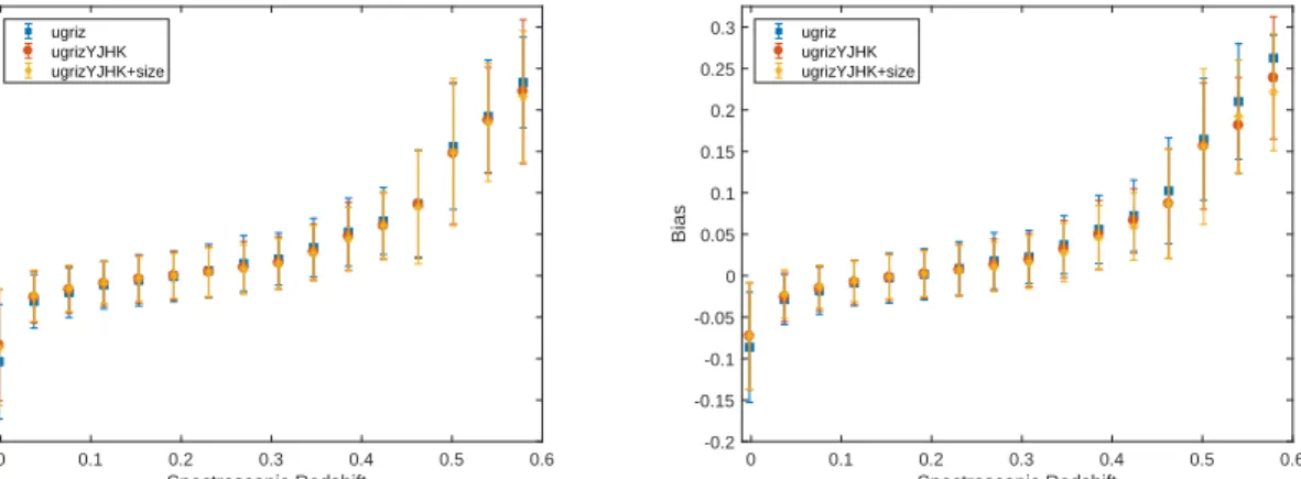
Figure 2. Bias versus redshift plots using the CSL methods normal (left) and normalized (right) and using ugriz, ugrizYJHK and ugrizYJHK filters with size data.
CSL Method Filters RMSE BIAS MLL FR0.15 FR0.05 Variance Model Var Noise Var
Normal ugriz 0.0393 -0.00228 1.79 99.35 85.08 0.0023 7.0E-06 0.0023 ugrizYJHK 0.0360 -0.00185 1.84 99.54 87.92 0.0018 6.5E-06 0.0018 ugrizYJHK+size 0.0347 -0.00177 1.91 99.50 89.61 0.0018 7.7E-06 0.0018 Normalized ugriz 0.0387 0.00069 1.73 99.38 85.09 0.0014 6.3E-06 0.0014 ugrizYJHK 0.0357 0.00031 1.80 99.53 87.77 0.0013 6.9E-06 0.0013 ugrizYJHK+size 0.0340 0.00048 1.85 99.55 89.87 0.0011 6.2E-06 0.0011
Table 2.Summary performance measures and variances for the CSL methods normal and normalized with ugriz filters, ugrizYJHK filters and ugrizYJHK filters and size data. The number of training, validation and testing objects are: 25574, 25575 and 12788 respectively. The best metrics and variances are highlighted.
Normal
Redshift Bin Ntrain Nvalid Ntest RMSE BIAS MLL FR0.15 FR0.05 Variance Model Var Noise Var
0-0.1 4592 4621 2297 0.0510 -0.0298 1.86 98.04 78.49 0.0020 9.2E-06 0.0020 0.1-0.2 11613 11442 5888 0.0309 -0.0063 2.02 99.92 89.93 0.0019 5.6E-06 0.0019 0.2-0.3 6809 6973 3366 0.0345 0.0095 1.73 99.88 86.54 0.0028 7.1E-06 0.0028 0.3-0.4 2117 2105 1012 0.0471 0.0313 1.25 99.31 74.41 0.0030 9.2E-06 0.0030 0.4-0.5 259 244 134 0.0954 0.0766 -2.20 91.04 37.31 0.0071 1.6E-05 0.0071 0.5-0.6 27 28 14 0.2012 0.1879 -10.22 35.71 0.00 0.0115 2.3E-05 0.0115 Normalized 0-0.1 4592 4621 2297 0.0460 -0.0263 1.86 98.65 81.15 0.0013 7.5E-06 0.0013 0.1-0.2 11613 11442 5888 0.0299 -0.0036 2.05 99.93 90.64 0.0013 5.1E-06 0.0012 0.2-0.3 6809 6973 3366 0.0357 0.0123 1.68 99.79 84.28 0.0017 6.4E-06 0.0017 0.3-0.4 2117 2105 1012 0.0493 0.0341 0.89 98.91 72.43 0.0018 8.6E-06 0.0018 0.4-0.5 259 244 134 0.1039 0.0858 -4.89 87.31 33.58 0.0036 1.6E-05 0.0036 0.5-0.6 27 28 14 0.2194 0.2067 -16.24 35.71 0.00 0.0054 2.2E-05 0.0054
Table 3.Table showing performance measures and variances by redshift bin for the CSL methods normal and normalized with ugriz filters. The best metrics and variances are highlighted.
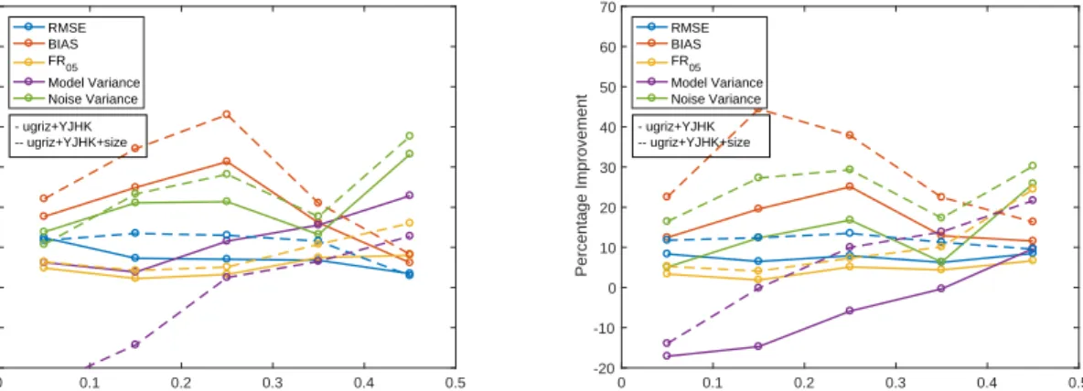
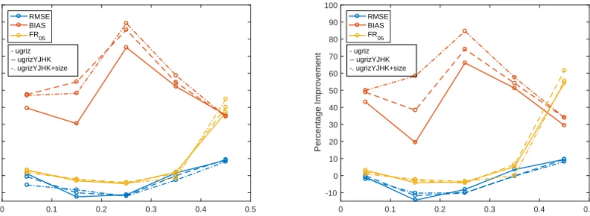
0 0.1 0.2 0.3 0.4 0.5 Redshift bin -20 -10 0 10 20 30 40 50 60 70 Percentage Improvement RMSE BIAS FR05 Model Variance Noise Variance - ugriz+YJHK -- ugriz+YJHK+size 0 0.1 0.2 0.3 0.4 0.5 Redshift bin -20 -10 0 10 20 30 40 50 60 70 Percentage Improvement RMSE BIAS FR05 Model Variance Noise Variance - ugriz+YJHK -- ugriz+YJHK+size
Figure 3.Percentage improvements of performance measures and variances by redshift bin due to the use of ugrizYJHK filters and size data using the normal (left) and normalized (right) methods. The solid lines represent the improvements due to adding the near-IR features and the dashed lines represent the improvements due to adding both the near-IR and angular size features.
from adding the near-IR followed by the angular size fea-tures. Improvements are clearly seen across all metrics in all redshift bins and apart from one case involving the model variance, the angular size features clearly provide signifi-cant added improvements compared to the near-IR features
alone. The RMSE and FR0.05 metrics both undergo smaller
improvements in regions with higher data densities, where the original estimates were more accurate, while they
in-crease more significantly (FR0.05in particular) in the lower
density regions. The bias appears to undergo significant im-provements over all redshift bins, but because the original
values were very small (seeTable 3), very small changes led
to large percentage improvements. Figure 2shows the bias
as a function of redshift, and here, a similar trend to the other metrics is observed: more significant improvements oc-cur in regions of lower number densities. Improvements of
FR0.15 (not shown) were negligible, while those of FR0.05
were more significant in all redshift bins, this implies that the addition of these features does not have a significant in-fluence on the worst outliers, but decreases the scatter of objects with smaller initial deviations.
0 0.5 1 1.5 2 Spectroscopic Redshift -0.1 0 0.1 0.2 0.3 0.4 0.5 Photometric Redshift -10 -9 -8 -7 -6 -5 -4 -3 Quasar/AGN
Figure 4.Plot showing the location of catastrophic outliers.
3.5 Outliers
When the entire redshift range for which data is present (z < 2.1) was studied, we identified those objects with the
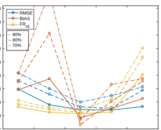
0 0.1 0.2 0.3 0.4 0.5 Redshift bin -10 0 10 20 30 40 50 60 70 80 Percentage Improvement RMSE BIAS FR05 - 90% -- 80% -. 70%
Figure 5.Percentage improvements of performance measures by redshift bin when 90, 80 and 70 per cent of the testing data with the lowest uncertainties were used. CSL method normal using ugrizYJHK filters and size data was used
of these objects were either quasars, narrow-line AGN or had noisy spectra that made it difficult to determine a redshift. In addition, although this set contained objects with a range
of redshifts, all the outliers with high redshifts (z > 0.55)
were contained in this group, the positions of these outliers
are shown inFigure 4.
The reason why theGPzalgorithm was unable to
cor-rectly predict the redshift of these quasars and AGN is be-cause too few of these were present in the training data to allow the algorithm to make realistic estimates. We see from the analysis in the previous section that the number of objects available for training in each bin is an important fac-tor in obtaining accurate estimates, thus if a large sample of quasars and other AGN was present, we expect that photo-z estimation of these objects would be greatly improved. For the objects with noisy spectra, the spectroscopic redshifts may have been incorrectly determined (as our constraint of
NQ ≤ 3 will not result in 100 per cent accuracy for the
spectroscopic redshifts), in which case the photometric red-shift estimate may be more accurate than the spectroscopic redshift.
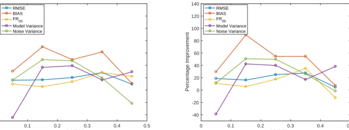
InFigure 5we show the improvement in metric perfor-mance as we reduce the sample according to the variance prediction. We see that as higher variance estimates are re-moved, our results improve greatly: cutting the values with higher uncertainties and using 90, 80 and 70 per cent of the test data with the lowest variances shows consistent im-provement in all metrics. This was using using ugrizYJHK filters and size data, but the same trend is observed us-ing only ugriz and ugrizYJHK filters. As this removal of data was based solely on the variance values, this method can also be used for real surveys to obtain appropriate sam-ples—based on the specifications for data density and vari-ance necessary for the specific science case.
4 Optimizing the Probability Density Functions
It has become clear that single point estimates of the pho-tometric redshifts are insufficient for many scientific appli-cations, and the full probability density function (PDF) is
preferred. However, it is extremely difficult to obtain reliable PDFs from both template fitting (due to non-representative templates) and empirical methods (where for example ab-sence of data is traditionally difficult to quantify). Some methods employ post-processing to give their estimated
PDFs the correct statistical properties (see Bordoloi et al.
2012; Polsterer et al. 2016), GPz overcomes this by intro-ducing an additional noise term to alleviate some of these issues.
In this section we investigate the accuracy of the proba-bility density functions (PDFs) of the photometric redshifts
using Quantile-Quantile (Q-Q) plots (as inWittman et al.
2016). We use these to provide appropriate alterations to
the PDFs with the aim of further optimizing the redshift estimates. The first step in doing this is calculating the per-centiles of the spectroscopic redshifts relative to the PDFs of the photometric redshifts. The PDF of the photo-z for a
given object obtained using theGPzalgorithm is Gaussian
with mean equal to the photo-z estimate and variance given by the sum of the model and noise variances. The percentile
of a given redshift (z1) is given by the value of the cumulative
distribution function (CDF) at that redshift [CDF(z=z1)].
In this way, the percentiles of every spec-z relative to the photo-z PDFs were calculated.
Next, the percentiles were used to determine the
quan-tiles: the quantile at a valuexis defined as the fraction of
percentiles that are below the fraction x(for example: the
quantile at 0.2 is given by the fraction of objects with per-centiles less than 0.2). Theoretically, for perfect sampling of
a distribution we expect that for all fractionsx(0< x <1),
quantile(x) =xas 20 per cent of values are expected to have
percentiles less than or equal to 0.2 and so on. The calculated quantiles versus the theoretical quantiles (Q-Q) are shown in
Figures 6aand6c. A Q-Q plot with a straight line indicates that the photometric redshift PDFs (and thus the means and variances) are appropriately representing the spectro-scopic redshift distribution, i.e. the spectrospectro-scopic redshift values are representative of a random sampling of the pho-tometric redshift PDFs. Deviations from this straight line indicate deviation from ideal photometric PDFs and this is
quantified using the Euclidean distance (ηn). ηn versus the
shift required for the PDF (e.g.Figure 6b) are then
deter-mined by applying multiple positive and negative shifts to the means of the PDFs, finding the respective percentiles of the spectroscopic redshifts, followed by the corresponding
quantiles, and then findingηn of the Q-Q plots. The p(z)
shift that minimizes theηn is then taken as the shift to be
applied to the photometric redshifts.
In this analysis, one half of the test data was used to
produceηnversusp(z) for each redshift bin in order to find
the optimalp(z) shift (Figure 6). Thesep(z) shifts were then
applied to all the best fit photometric redshift values in the respective photometric redshift bins of the second half of the test data. Half of the test data was used instead of the entire set and the shifts were applied in photo-z instead of spec-z bins in order to illustrate the utility of this method when spectroscopic data is present for only a subset of the data. All spectroscopic redshifts with percentiles equal to 0 or 1 were not used for producing the Q-Q plots, as the corresponding photo-z’s—defining the relevant PDFs—are considered to be outliers. The fraction of sources not within
0 0.1 0.2 0.3 0.4 0.5 0.6 0.7 0.8 0.9 1 QTheory 0 0.1 0.2 0.3 0.4 0.5 0.6 0.7 0.8 0.9 1 QModel fout=0 n=4.2577 Redshift bin:0.3-0.4 Model Ideal
(a) Before shift
-0.4 -0.3 -0.2 -0.1 0 0.1 0.2 0.3 p(z) shift 0 1 2 3 4 5 6 7 8 9 10 n 0.035726, 0.29133 Redshift bin:0.3-0.4 (b)ηnvsP(z) 0 0.1 0.2 0.3 0.4 0.5 0.6 0.7 0.8 0.9 1 QTheory 0 0.1 0.2 0.3 0.4 0.5 0.6 0.7 0.8 0.9 1 QModel fout=0 n=0.29133 Redshift bin:0.3-0.4 Model Ideal (c) After shift
Figure 6. (a) Q-Q plot in the redshift bin 0.3-0.4 with the CSL method normal using ugriz filters before applying shifts, (b) the correspondingηnvsP(z) and (c) the Q-Q plot after thep(z) shift was applied.
0 0.1 0.2 0.3 0.4 0.5 Redshift bin -10 0 10 20 30 40 50 60 70 80 90 100 Percentage Improvement RMSE BIAS FR05 - ugriz -- ugrizYJHK -. ugrizYJHK+size 0 0.1 0.2 0.3 0.4 0.5 Redshift bin -10 0 10 20 30 40 50 60 70 80 90 100 Percentage Improvement RMSE BIAS FR05 - ugriz -- ugrizYJHK -. ugrizYJHK+size
Figure 7.Percentage improvements of performance measures by redshift bin due to shifting the means of the photo-z PDFs compared to before the means were shifted using the same training, validation and testing objects and using the normal (left) and normalized (right) methods.The solid lines represent using the ugriz features, the dashed line represents using the ugrizYJHK features and the dash-dotted line represents using the ugrizYJHK and angular size features.
outliers divided by the number of objects in the relevant
redshift bin. In this analysis, thefoutafter applying thep(z)
shifts was 0 in all bins considered (0-0.5) apart from the
0.4-0.5 bin in which the fout did not surpass 0.05 which
corresponds to 3 objects.
The Q-Q plots obtained after applying the photo-z shifts in all redshift bins were near to straight lines, with
very lowηnvalues. This means that theGPzalgorithm
pro-duced appropriate variance estimates with a slight bias on the mean values. The optimal shifts found were very small in redshift bins with large numbers of data points, mean-ing that the mean values produced in these bins were accu-rate. On the other hand, the shifts were significant in the
redshift bins with lower densities (seeFigure 6), indicating
that some bias was present in these bins but that this post-processing method was able to adjust the positions of the PDFs such that they were more representative of the
spec-troscopic redshifts. Curves like the one shown in Figure 6a
which represent a lack of objects with percentiles below the given fraction for all quantiles, correspond to the PDFs gen-erally being biased to low redshifts and thus a shift to higher
redshift is suggested by theηn vsp(z) plot. Q-Q plots that
indicated that the PDFs were biased to low redshift were
obtained for the higher redshift bins (z >0.2) while the
op-posite was obtained for the lower redshift bins (z < 0.1).
This can be explained by the fact that the best fit mean function will be found where the data density is highest,
which is around the redshift of z ∼ 0.2. In some redshift
bins (e.g.z >0.5) the number of galaxies was too small for
this analysis to be carried out.
Figure 7gives the percentage improvements of the per-formance metrics by redshift bin due to shifting the PDFs (the variances are not included as they are not affected by the shifts). For all the redshift bins in which this method was
applied (z < 0.5), for all configurations of input variables
and for both CSL methods we see significant improvement in the bias metric, while the other metrics only worsen slightly in some redshift bins. The bias shows the most significant improvements because this method of using the Q-Q plots to shift the PDFs specifically targets the bias. The RMSE
and FR0.05metrics both show improvements in redshift bins
with lower number densities, while improvements are mini-mal in the highest density bins. This is because the original model was such that it fit the more dense regions better than the less dense ones, resulting in biases on both sides of the central dense region. These clear improvements demonstrate the efficiency of this post-processing method and we expect further improvements if smaller redshift bins are used.
5 Effects of Improved Photometry
In this section we investigate and quantify the improvement in the photometric redshifts with deeper imaging data over a subset of the GAMA fields used thus far.
The Hyper Suprime-Cam Subaru Strategic Program
(HSC-SSP) Data Release 1(Aihara et al. 2017) provides
photometry in grizy filters with magnitude errors that are an order of magnitude smaller than the SDSS/UKIDSS LAS photometry. We crossmatched the positions of the galaxies used for the previous analyses with the HSC galaxies and combined the corresponding photometry with the GAMA
spectroscopy. After eliminating spec-z’s with NQ<3 and
re-moving any objects with missing SDSS/UKIDSS LAS or HSC photometry we found that only 20253 GAMA objects were matched to HSC objects. This was because only limited portions of the GAMA fields were covered in the HSC-SSP
survey (seeAihara et al. 2017).
TheGPzalgorithm with 100 basis functions and
mod-elling of heteroscedastic noise was then used to estimate the photometric redshifts from both the HSC grizy photome-try and the SDSS/UKIDSS LAS grizY photomephotome-try for an identical set of galaxies. It should be noted that the Y filter from the UKIDSS LAS photometry is of a different shape to the y filter from the HSC photometry, but they are similar enough to be used for comparison. Photometric redshift
ver-sus spectroscopic redshift plots are shown in Figure 8, the
percentage improvements of the performance measures and
variances by redshift bin are shown inFigure 9, and metrics
are given inTable 4. It is evident from these figures that the
HSC photometry produces a tighter distribution than the SDSS/UKIDSS LAS photometry, and the metrics showing significant improvements when the HSC data is used. In ad-dition to improved metrics, the model and noise variances are also improved. As previously discussed, improved preci-sion of the input data should decrease the noise variance as the spread of the data should decrease. The model variance also improves as the algorithm is much more confident about the model fit with the more precise data.
Next, all available filters as well as size data were added
to the estimates obtained using the GPz algorithm from
the GAMA SDSS/UKIDSS LAS dataset. The results are
summarized in Table 4. We see that although the HSC
data clearly outperforms the SDSS/UKIDSS LAS data when only five filters are used, it does very similarly to the SDSS/UKIDSS LAS data when near-IR data are added and is outperformed in most metrics by a small margin when size data is also added.
Considering the limited size of the data set, the im-provements in the metrics provided by the improved quality of the photometry are very significant and thus, further im-provements in photometry over large survey regions—as will be provided by future surveys such as the Large Synoptic
Survey Telescope (LSST;LSST Science Collaboration et al.
2009) andEuclid(Laureijs et al. 2011)—will have significant
impacts on the ability of the GPz algorithm to accurately
predict the photometric redshifts of galaxies.
6 Conclusions
In this paper, methods of obtaining improved
photomet-ric redshift estimations from theGPzmachine learning
al-gorithm were investigated. These methods were introduc-ing near-IR magnitudes and angular size features, post-processing the results by shifting the photo-z estimates based on their Q-Q plots and utilizing photometry with higher precision. It was found that the inclusion of near-IR (YJHK) filters and angular size data in the training, val-idation and testing of photometric redshift estimation re-sulted in significantly improved accuracy, and thus, when available, this data should be utilized. The process of shift-ing the probability distributions of the estimated redshifts
by minimizing theηn value has proven to substantially
im-prove the bias of the estimated photometric redshifts. There-fore, when a suitable spectroscopic sample is available, this method could be applied to supply additional accuracy to
the predictions fromGPzand other methods. Finally, we see
that improvements in the accuracy of the photometry im-proved the accuracy of the photometric redshifts, to a very similar extent as adding the near-IR and angular size data, and therefore, work should continue to be done to improve the quality of the photometric data obtained.
It is worth mentioning that we have targeted galaxies
predominantly at z < 0.5 in this study, where one might
expect the size information to have more of an influence, but where one might also expect the near-infrared filters to add a comparatively smaller amount of information compared to z >1, where the 4000˚A break moves out of the visible wavelength filters. In a future paper we will explore this issue by combining the deeper visible wavelength data (e.g.
Aihara et al. 2017) with deeper near-infrared data over the well studied extragalactic deep fields.
Acknowledgements
ZG is supported by a Rhodes Scholarship granted by the Rhodes Trust. IAA would like to acknowledge the support of King Abdulaziz City for Science and Technology.
GAMA is a joint European-Australasian project based around a spectroscopic campaign using the Anglo-Australian Telescope. The GAMA input catalogue is based on data taken from the Sloan Digital Sky Survey and the UKIRT Infrared Deep Sky Survey. Complementary imaging of the GAMA regions is being obtained by a number of in-dependent survey programmes including GALEX MIS, VST KiDS, VISTA VIKING, WISE, Herschel-ATLAS, GMRT and ASKAP providing UV to radio coverage. GAMA is funded by the STFC (UK), the ARC (Australia), the AAO, and the participating institutions. The GAMA website is http://www.gama-survey.org/.
The Hyper Suprime-Cam (HSC) collaboration includes the astronomical communities of Japan and Taiwan, and Princeton University. The HSC instrumentation and soft-ware were developed by the National Astronomical Obser-vatory of Japan (NAOJ), the Kavli Institute for the Physics and Mathematics of the Universe (Kavli IPMU), the Uni-versity of Tokyo, the High Energy Accelerator Research Or-ganization (KEK), the Academia Sinica Institute for As-tronomy and Astrophysics in Taiwan (ASIAA), and Prince-ton University. Funding was contributed by the FIRST pro-gram from Japanese Cabinet Office, the Ministry of Educa-tion, Culture, Sports, Science and Technology (MEXT), the Japan Society for the Promotion of Science (JSPS), Japan
0 0.1 0.2 0.3 0.4 0.5 0.6 Spectroscopic Redshift -0.1 0 0.1 0.2 0.3 0.4 0.5 0.6 Photometric Redshift -9 -8 -7 -6 -5 -4 Normal SDSS/UKIDSS 0 0.1 0.2 0.3 0.4 0.5 0.6 Spectroscopic Redshift -0.1 0 0.1 0.2 0.3 0.4 0.5 0.6 Photometric Redshift -9 -8 -7 -6 -5 -4 Normal HSC 0 0.1 0.2 0.3 0.4 0.5 0.6 Spectroscopic Redshift -0.1 0 0.1 0.2 0.3 0.4 0.5 0.6 Photometric Redshift -9 -8 -7 -6 -5 -4 SDSS/UKIDSS Normalized 0 0.1 0.2 0.3 0.4 0.5 0.6 Spectroscopic Redshift -0.1 0 0.1 0.2 0.3 0.4 0.5 0.6 Photometric Redshift -10 -9 -8 -7 -6 -5 HSC Normalized
Figure 8.Photometric redshift versus spectroscopic redshift plots showing the performance of theGPzcode using SDSS/UKIDSS LAS photometry (left) and HSC photometry (right) with the CSL methods normal and normalized (in the first and second rows respectively). The colour scale represents the variance of data points in that area of the plot and the straight line is thez= ˆzline.
CSL Method Survey Features RMSE BIAS MLL FR0.15 FR0.05 Variance Model Var Noise Var
Normal SDSS/ grizY 0.0432 -0.0013 1.70 99.18 81.25 0.0025 2.3E-05 0.0025
UKIDSS LAS ugrizYJHK 0.0352 -0.0014 1.87 99.60 88.22 0.0018 2.1E-05 0.0018 ugrizYJHK+size 0.0336 -0.0012 1.92 99.53 89.64 0.0016 2.1E-05 0.0016
HSC grizy 0.0357 -0.0008 1.94 99.33 89.14 0.0015 1.9E-05 0.0015
Normalized SDSS/ grizY 0.0432 0.0021 1.64 99.25 80.67 0.0018 2.3E-05 0.0018
UKIDSS LAS ugrizYJHK 0.0355 0.0010 1.83 99.58 88.17 0.0014 2.2E-05 0.0013
ugrizYJHK+size 0.0334 0.0007 1.87 99.55 89.86 0.0011 1.9E-05 0.0011
HSC grizY 0.0349 0.0011 1.85 99.43 89.64 0.0011 1.8E-05 0.0010
Table 4.Table showing summary performance measures and variance for the HSC photometry with grizy filters and the SDSS/UKIDSS LAS photometry with all three configurations of features. The number of training, validation and testing objects are: 8047, 8048 and 4024 respectively. The best metrics and variances are highlighted.
Science and Technology Agency (JST), the Toray Science Foundation, NAOJ, Kavli IPMU, KEK, ASIAA, and Prince-ton University.
This paper makes use of software developed for the Large Synoptic Survey Telescope. We thank the LSST Project for making their code available as free software at http://dm.lsstcorp.org.
The Pan-STARRS1 Surveys (PS1) have been made possible through contributions of the Institute for Astron-omy, the University of Hawaii, the Pan-STARRS Project Office, the Max-Planck Society and its participating insti-tutes, the Max Planck Institute for Astronomy, Heidelberg and the Max Planck Institute for Extraterrestrial Physics, Garching, The Johns Hopkins University, Durham Univer-sity, the University of Edinburgh, Queens University Belfast, the Harvard-Smithsonian Center for Astrophysics, the Las Cumbres Observatory Global Telescope Network Incorpo-rated, the National Central University of Taiwan, the Space
Telescope Science Institute, the National Aeronautics and Space Administration under Grant No. NNX08AR22G is-sued through the Planetary Science Division of the NASA Science Mission Directorate, the National Science Founda-tion under Grant No. AST-1238877, the University of Mary-land, and Eotvos Lorand University (ELTE) and the Los Alamos National Laboratory.
Based [in part] on data collected at the Subaru Tele-scope and retrieved from the HSC data archive system, which is operated by Subaru Telescope and Astronomy Data Center, National Astronomical Observatory of Japan.
REFERENCES
Abdalla F. B., Banerji M., Lahav O., Rashkov V., 2011,MNRAS,
417, 1891
Aihara H., et al., 2017, preprint, (arXiv:1702.08449) Alam S., et al., 2016, preprint, (arXiv:1607.03155)
0 0.1 0.2 0.3 0.4 0.5 Redshift bin -40 -20 0 20 40 60 80 100 120 140 Percentage Improvement RMSE BIAS FR05 Model Variance Noise Variance 0 0.1 0.2 0.3 0.4 0.5 Redshift bin -40 -20 0 20 40 60 80 100 120 140 Percentage Improvement RMSE BIAS FR05 Model Variance Noise Variance
Figure 9.Percentage improvements of performance measures and variances by redshift bin due to the use of HSC grizy filters compared to SDSS/UKIDSS LAS grizY filters using the same training, validation and testing objects and using the normal (left) and normalized (right) methods.
Almosallam I. A., Lindsay S. N., Jarvis M. J., Roberts S. J., 2016a,MNRAS,455, 2387
Almosallam I. A., Jarvis M. J., Roberts S. J., 2016b,MNRAS,
462, 726
Banerji M., et al., 2010,MNRAS,406, 342
Baum W. A., 1962, in McVittie G. C., ed., IAU Symposium Vol. 15, Problems of Extra-Galactic Research. p. 390
Ben´ıtez N., 2000,ApJ,536, 571
Ben´ıtez N., et al., 2009,ApJ,692, L5
Bernstein G., Huterer D., 2010,MNRAS,401, 1399
Blake C., Collister A., Bridle S., Lahav O., 2007, MNRAS,
374, 1527
Blake C., et al., 2011,MNRAS,415, 2876
Bolzonella M., Miralles J.-M., Pell´o R., 2000, A&A,363, 476
Bordoloi R., et al., 2012,MNRAS,421, 1671
Brammer G. B., van Dokkum P. G., Coppi P., 2008, ApJ,
686, 1503
Bridle S., King L., 2007,New Journal of Physics,9, 444
Budav´ari T., Szalay A. S., Connolly A. J., Csabai I., Dickinson M., 2000,AJ,120, 1588
Budav´ari T., Szalay A. S., Csabai I., Connolly A. J., Tsvetanov Z., 2001,AJ,121, 3266
Carrasco Kind M., Brunner R. J., 2013,MNRAS,432, 1483
Chambers K. C., et al., 2016, preprint, (arXiv:1612.05560) Cole S., et al., 2005,MNRAS,362, 505
Colless M., et al., 2001,MNRAS,328, 1039
Collister A. A., Lahav O., 2004,PASP,116, 345
Connolly A. J., Csabai I., Szalay A. S., Koo D. C., Kron R. G., Munn J. A., 1995,AJ,110, 2655
Dawson K. S., et al., 2013,AJ,145, 10
Feldman H. A., Kaiser N., Peacock J. A., 1994,ApJ,426, 23
Feldmann R., et al., 2006,MNRAS,372, 565
Firth A. E., Lahav O., Somerville R. S., 2003,MNRAS,339, 1195
Fu L., et al., 2008,A&A,479, 9
Fukugita M., Ichikawa T., Gunn J. E., Doi M., Shimasaku K., Schneider D. P., 1996,AJ,111, 1748
Gauci A., Zarb Adami K., Abela J., 2010, preprint, (arXiv:1005.0390)
Hickson P., Gibson B. K., Callaghan K. A. S., 1994, MNRAS,
267, 911
Hildebrandt H., et al., 2010,A&A,523, A31
Hogan R., Fairbairn M., Seeburn N., 2015,MNRAS,449, 2040
Hong T., Han J. L., Wen Z. L., Sun L., Zhan H., 2012, ApJ,
749, 81
Hoyle B., Rau M. M., Zitlau R., Seitz S., Weller J., 2015,MNRAS,
449, 1275
Ilbert O., et al., 2006,A&A,457, 841
Ilbert O., et al., 2015,A&A,579, A2
Jain B., Taylor A., 2003,Physical Review Letters,91, 141302
Jeong D., Dai L., Kamionkowski M., Szalay A. S., 2015,MNRAS,
449, 3312
Johnston R., Vaccari M., Jarvis M., Smith M., Giovannoli E., H¨außler B., Prescott M., 2015,MNRAS,453, 2540
Koo D. C., 1985,AJ,90, 418
LSST Science Collaboration et al., 2009, preprint, (arXiv:0912.0201)
Laureijs R., et al., 2011, preprint, (arXiv:1110.3193)
Li L.-L., Zhang Y.-X., Zhao Y.-H., Yang D.-W., 2007,
Chinese J. Astron. Astrophys.,7, 448
Lilly S. J., et al., 2009,ApJS,184, 218
Lin H., Hao C., Wang X., Yuan Q., Yi Z.-L., Zhang T.-J., Wang B.-Q., 2009,Modern Physics Letters A,24, 1699
Liske J., et al., 2015,MNRAS,452, 2087
Mobasher B., et al., 2004,ApJ,600, L167
Oyaizu H., Lima M., Cunha C. E., Lin H., Frieman J., Sheldon E. S., 2008,ApJ,674, 768
Polsterer K. L., D’Isanto A., Gieseke F., 2016, preprint, (arXiv:1608.08016)
Rasmussen C. E., Williams C. K. I., 2006, Gaussian Processes for Machine Learning. The MIT Press
Rudnick G., et al., 2001,AJ,122, 2205
S´anchez C., et al., 2014,MNRAS,445, 1482
Seo H.-J., Eisenstein D. J., 2003,ApJ,598, 720
Singal J., Shmakova M., Gerke B., Griffith R. L., Lotz J., 2011,
PASP,123, 615
Tagliaferri R., Longo G., Andreon S., Capozziello S., Donalek C., Giordano G., 2003, Lecture Notes in Computer Science,
2859, 226
Tanaka M., et al., 2017, preprint, (arXiv:1704.05988)
The Dark Energy Survey Collaboration 2005, ArXiv Astrophysics e-prints,
Vargas-Maga˜na M., et al., 2016, preprint, (arXiv:1610.03506) Wang Y., Bahcall N., Turner E. L., 1998,AJ,116, 2081
Way M. J., 2011,ApJ,734, L9
Wittman D., Bhaskar R., Tobin R., 2016,MNRAS,457, 4005
de Jong J. T. A., Verdoes Kleijn G. A., Kuijken K. H., Valentijn E. A., 2013,Experimental Astronomy,35, 25
This paper has been typeset from a TEX/LATEX file prepared by the author.