Ratio maps and correspondence analysis

Ratio Maps and Correspondence Analysis

Michael Greenacre

Universitat Pompeu Fabra, Barcelona, Spain

Summary. We compare two methods for visualising contingency tables and develop a method called the ratio map which combines the good properties of both. The first is a biplot based on the logratio approach to compositional data analysis. This approach is founded on the principle of subcompositional coherence, which assures that results are invariant to considering subsets of the composition. The second approach, correspondence analysis, is based on the chi-square approach to contingency table analysis. A cornerstone of correspondence analysis is the principle of distributional equivalence, which assures invariance in the results when rows or columns with identical conditional proportions are merged. Both methods may be described as singular value decompositions of appropriately transformed matrices. Correspondence analysis includes a weighting of the rows and columns proportional to the margins of the table, If this idea of row and column weights is introduced into the logratio biplot, we obtain a method which obeys both principles of subcompositional coherence and distributional equivalence.

Keywords: Biplot; compositional data; contingency tables; correspondence analysis; distribu-tional equivalence; logratio transformation; singular value decomposition; spectral map.

SOUTH AFRICAN VERSION - WORKING PAPER IN PROGRESS

1_{This research has been supported by Spanish Ministry of Science and Technology grant}

BFM2000-1064. Address for correspondence: Michael Greenacre, Department of Economics, Universitat Pompeu Fabra, Ramon Trias Fargas 25–27, 08005 Barcelona, Spain. E-mail: [email protected].

1

Introduction

This article considers different ways of visualizing contingency tables in the form of a map, where the rows and columns of the table are depicted as points in a low-dimensional Euclidean space, usually a two-dimensional plane. As a special case we shall look at tables of compositional data, that is positive data with row sums (or column sums) equal to a constant, usually 1 if the data are proportions or 100 if they are percentages. A method called the ratio map is introduced, which can be considered as a type of fusion of ideas emanating from compositional data analysis and correspondence analysis.

Correspondence analysis (Benz´ecri, 1973; Greenacre, 1984, 1993) has become a popular method for graphically displaying tables of nonnegative data, applicable primarily to contingency tables. The method, popular in the social and environmental sciences, has several equivalent definitions. One definition, in a nutshell, is the following (see, for example, Greenacre 1993). First, transform the rows of the table into profiles, that is the rows divided by their row totals. Second, assign weights to the row profiles proportional to the marginal row totals of the contingency table (these weights which sum to 1 are called “masses” in correspondence analysis). Third, perform a standardization of the profile elements by dividing them by values proportional to the square root of the marginal column totals of the contingency table. The third step implies a special distance function between the profiles, called thechi-squared distance. Finally, perform a weighted principal component analysis on the row profiles, identifying the plane, for example, which best fits the row profiles by minimizing the weighted sum of squared (chi-squared) distances from the points to the plane. Then project the profile points onto this plane and interpret their relative positions. An identical and completely symmetric analysis can be performed of the column profiles, and the two analyses are equivalent in that their solutions are based on the singular value decomposition (SVD) of the same matrix (Greenacre, 1984).

As emphasised often by Benz´ecri, who originally developed correspondence analysis as a method for exploring large frequency tables in linguistics, one of the founding principles of the method is the principle of distributional equivalence: “Our first principle is that

of distributional equivalence” (Benz´ecri, 1973, vol.I, p. 23). This principle can be stated simply as follows: if two rows (or two columns) have the same relative values, that is they have the same profile, then merging them does not affect the results in any way. As an illustration of this principle, suppose that words have been counted in a sample of texts, including the two articles “the” and “a”, and that the frequencies are collected in a texts×words table. Suppose that it turns out that in each text, the relative occurrence of these two articles is identical, for example “a” always occurs 25% of the times “the” occurs. This means that the (column) profile of “a” is identical to that of “the”. The principle of distributional equivalence states that it should make no difference to the analysis if we merge two such columns with identical profiles, adding together the frequencies to obtain one column, which could be labelled “articles” and where we make no distinction between its two components.

Geometrically, two identical profiles are points lying at identical positions and the result of the merger is a single point with mass equal to the sum of the masses. Trivially, it is clear that all distances between column profiles are unaffected by this merger, since the row margins are unaffected by the merger and thus all interpoint column distances stay the same. Less trivially, however, the chi-squared distances between all text (row) points is also unaffected, thus assuring distributional equivalence (for a proof, see Greenacre, 1984, section 4.1.17). The principle of distributional equivalence similarly guarantees invariance of all results if a row (or column) were split into parts in constant proportions. For example, if one column is split into three columns in fixed proportions 70:20:10, the interpoint row distances remain invariant, as well as the correspondence analysis solution. Compositional data analysis (Aitchison, 1986) is concerned with data vectors of non-negative values summing to one. This methodology has become popular in the physical sciences, especially geology and chemistry, rather than the social sciences. For exam-ple, chemical samples are typically analyzed into constituent components by weight, or volume, expressed as proportions of the total sample. One of the founding principles of compositional data analysis is that ofsubcompositional coherence. Suppose that a chemi-cal sample has inorganic and organic components, and that scientist A is investigating all

of these components, whereas scientist B is investigating just the organic components of the same samples, that is B’s data are the organic components expressed as proportions of total organic material. Subcompositional coherence means that statistical analysis by scientist B on the subcomposition of organic components should be the same as that of scientist A, unaffected by the fact that B is looking at a reduced data set. This principle has led to the study of ratios of the components, which are clearly unaffected by looking at subcompositions.

Aitchison (1986) defined a variant of principal component analysis for compositional data, based on logarithmically transforming the component ratios, calledlogratios. Later Aitchison (1990) introduced the biplot associated with this approach, calling it the “rel-ative variation biplot”, displaying both the samples (usually rows) and the components (columns) in a joint map. This biplot has several interesting properties, summarized by Aitchison and Greenacre (2001), who show that it is equivalent to analyze all the pairwise logratios or to analyze the logarithms of the components for each sample relative to their geometric mean. Computationally, the relative variation biplot is derived directly from the SVD of the components which have been first logarithmically transformed and then double-centred with respect to row and column means. This methodology can be applied in exactly the same way to crosstabulations and other tables of counts. But although the relative variation biplot has subcompositional coherence, it does not have distributional equivalence. This is unfortunate for compositional data analysis, because if two compo-nents were always occurring in the same proportion in every sample, then the analysis should be unaffected by considering these two components taken as one. Or, putting this in a different way in another context, suppose we were measuring the proportion of species in a biological sample, and later decided to distinguish between males and females of each species. Then if the male-to-female ratio were actually constant within each species across all samples, there should be no change at all to our analysis whether we distinguished between male and female or not, since no new information is introduced at all apart from the constant sex ratio.

do not have the basic properties of the other: the logratio biplot in compositional data analysis has subcompositional coherence but not distributional equivalence, whereas cor-respondence analysis has the latter but not the former. We will show, however, that the simple introduction of the correspondence analysis concept of row and column weighting into the logratio biplot leads to a method of visualization that has both subcompositional coherence and distributional equivalence. This method, which we call the ratio map, can be used to analyze contingency tables as well as compositional data. As far as analyzing positive compositional data is concerned, the ratio map is a significant improvement over existing methods. As far as analyzing contingency tables is concerned, the ratio map forms an interesting alternative correspondence analysis, and could enjoy much wider use outside the natural sciences. But it does have a few disadvantages, for example zero fre-quencies are problematic since the data are log-transformed, and zero frefre-quencies occur frequently in the social and environmental sciences.

In section 2 the ratio map is defined in the context of contingency table analysis. In section 3 the map’s properties are listed and illustrated in the context of an application. Section 4 deals with the special case of compositional data and Section 5 closes with a comparison with correspondence analysis.

2

The ratio map

Suppose that N = {nij} denotes an I ×J contingency table, with row totals, column

totals and grand total denoted by ni+, n+j and n++ respectively. Let ri = ni+/n++

and cj =n+j/n++ be the respective row and column masses. Let r be the vector of row

masses,cthe vector of column masses andDrandDcthe corresponding diagonal matrices.

Denote by L the matrix of logarithms of the frequencies, `ij = log(nij). Aitchison’s

relative variation biplot consists of double-centring the matrix L with respect to simple arithmetic averages of the rows and columns, followed by a SVD to obtain least-squares matrix approximations. In the ratio map the row and column masses are introduced into the double-centring stage, so that centring is with respect to weighted averages, as

well as into the matrix approximation stage, so that fitting is by weighted least squares. This simple modification of the algorithm, giving differential importances to the rows and columns in the centring and fitting, will be shown to bestow on the method the principle of distributional equivalence.

The computational steps to find the coordinates of the rows and columns in the ratio map are as follows:

Step 1. Double-centre the matrix L with respect to its weighted row and column averages, the order of centring being invariant. That is, calculate the weighted averages of the rows ofL, using the column masses to weight each column element: `i·=

P

jcj`ij (i=

1, . . . , I), and then subtract these averages from all the elements in the corresponding row. Then centre the resultant matrix, with general element `ij−`i·, with respect to weighted

averages of the columns, using the row masses to weight each element: P_iri(`ij −`i·)

(j = 1, . . . , J), and then subtract these averages from all the elements in the corresponding columns. The result of this operation is a double-centred matrix with elements zij =`ij−

`i·−`·j+`··, where the dot subscript indicates weighted averaging over the corresponding

subscript. In matrix notation, this double-centring can be written as:

Z = (I−1rT)L(I−c1T)

Step 2. Multiply zij by (ricj)1/2, that is multiply the rows and columns by the square

root of their respective masses:

S=D1_r/2ZD1_c/2 Step 3. Perform the SVD of this transformed matrix:

S=UΓVT where UTU=VTV=I

and singular values in descending order: γ1 ≥γ2 ≥ · · ·>0.

Step 4. Divide the rows of the matrix of left singular vectors by r_i1/2, and divide the rows of the matrix of right singular vectors by c1_j/2:

f

Step 5. The rows of the matrices fU and Vf are the standard coordinates of the rows and columns respectively, while the same coordinates scaled by the corresponding singular values define the principal coordinates (Greenacre, 1984, 1993):

Principal coordinates Standard coordinates

Rows : F=UfΓ fU

Columns : G=fVΓ fV

As in all methods of this type, we can choose to represent either of two so-called asym-metric maps, using either F and fV for the asymmetric map which is “row-principal” or “row-metric-preserving”, orfUandGfor the asymmetric map which is “column-principal” or “column-metric-preserving”; or, alternatively, thesymmetric map usingFandGwhere both rows and columns are in principal coordinates. The asymmetric maps are biplots in the strict sense (Gabriel, 1971), but not the symmetric map (see, for example, Greenacre (1993)). Sometimes we use another symmetric solution which is a biplot, which we refer to as the symmetric biplot, with row coordinates ˜UΓ1/2 _{and column coordinates ˜VΓ}1/2_.

The symmetric biplot, however, favours neither the rows nor the columns in the strict sense of preserving the metric between rows or between columns.

Steps 2 to 4 are what Greenacre (1984) has called the “generalized singular value decomposition”, with row and column weights given by the row and column masses. These steps are equivalent to the following single step in which the singular vectors are constrained to have a weighted normalization.

Steps 2–4. Perform the generalized SVD of Z:

Z=fUΓfVT _whereUfT_D

rfU=fVTDcVf=I

In this weighted version of the SVD, low-rank approximations of the matrixZare weighted least-squares approximations, where the rows and columns are weighted by their corre-sponding row masses. This is exactly what is done in correspondence analysis, where the matrix being approximated by weighted least squares has elements (nij−ni+n+j)/(ni+n+j).

This is the only algorithmic difference between correspondence analysis and the ratio map. In Section 5 we shall comment in more detail on this relationship with correspondence analysis.

3

Application and properties of the ratio map

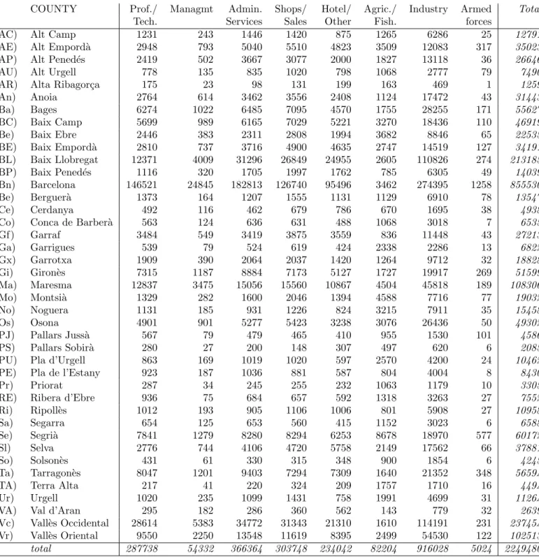
Consider the contingency table in Table 1, the frequencies of eight occupational categories in each of the 41 Catalan counties (comarcas). The table appears in Vives and Villarroya (1996) and the original source of the data is the Institut d’Estad´ıstica de Catalunya. This is an interesting table for our present purpose since it has rows and columns of widely differing totals, so the effect of weighting will be of relevance.

Insert Table 1 about here

The asymmetric ratio map favouring the display of the rows is given in Figure 1. In the terminology of Aitchison and Greenacre (2001) this type of asymmetric map is also called the form biplot.

Insert Figure 1 about here

We now list all the properties of a ratio map, using this example as an illustration. Vectors drawn from the origin of the display to a point are called rays, and vectors joining two row points or two column points are called links.

Property 1. The row points and column points are both centred in terms of weighted averages at the origin. This is a direct consequence of the weighted double-centring transformation of the matrix. Thus the weighted average row point in the display is at the origin and the weighted average column point as well. For example, in Figure 1 the origin is clearly not at the ordinary average row point, but well to the right because of the large mass of the point Bn(Barcelona).

Property 2. The ratio map, based on the SVD of a double-centred matrix, optimally represents the all inter-row differences and inter-column differences. This result has been shown for the unweighted case by Aitchison and Greenacre (2001, Appendix 1), who point out that it is really these differences which are of interest, and that the computational algorithm using the centred logratios is just a short cut to the analysis of all differences. For example, in Figure 1 the rays (1) and (3) indicate the directions of the biplot axes

for the columns “Professional/Technical” and “Services/Administration” respectively. If we are interested in the ratio between these two categories, then we simply look at the direction of the link connecting (1) and (3), which is practically vertical. From this we can deduce thatPS(Pallars Sobir`a) has one of the highest values of this ratio (from Table 1 it is 280/200=1.400) and BL (Baix Llobregat) one of the lowest (12371/31296=0.395). All the ratios between pairs of categories will be optimally displayed in this way.

Another way of thinking of this which is particularly useful in the case of contingency tables is to consider the matrix Y with 1

2n(n−1) rows and 12p(p−1) columns, having

general element yii0_,jj0 = log à nijni0_j0 nij0n_i0_j !

that is, the log-transformed odds ratio based on the four elements in rows i, i’ and columnsj, j0_{. If we assign weightsr}

iri0 to the rows andc_jc_j0 to the columns, and perform

a weighted SVD as before, this is equivalent to performing a singular value decomposition of the smaller I×J matrixZ of double-centred log-frequencies, as in the ratio map. The total sum of squares is identical, the singular values are identical and the map coordinates of the rows or columns of Y may be obtained from the differences in the corresponding coordinates of the respective row or column pairs in the ratio map. Thus the ratio map is optimally displaying all the odds ratios that can be calculated on the contingency table and a particular odds ratio can be estimated by considering the two links connecting the pair of rows and pair of columns.

In other words, in the ratio map not only are the points themselves optimally displayed but also all the links are optimal representations of the true links in higher-dimensional space. The proof of this result is very similar to that given by Aitchison and Greenacre (2001), with the variation of including the weights in the process of fitting.

Property 3. Distances between row points and between column points in principal coordinates are approximations ofweighted Aitchison distancesbetween rows and between columns. These distances are defined in terms of the logarithms of ratios between data values. Consider, for example, the distances between row points i and i0_{, corresponding}

to rows [ni1ni2 . . . nip] and [ni0₁n_i0₂ . . . n_i0_p] of the data matrix. Each row ofJ elements

can be re-expressed as the set of 1

2J(J−1) ratios between all pairs of elements, for example

ni1/ni2,ni1/ni3, ni2/ni3, ... and so on, that is the ratios nij/nij0 forj < j0. This vector of

ratios describes the corresponding row, and since these ratios are considered to be on a multiplicative scale they are logarithmically transformed to logratiosτi,jj0 = log(n_ij/n_ij0).

If the columns are not differentially weighted, the Aitchison distance between two rows is proportional to the Euclidean distance between the vectors of logratios τi = [τi,jj0] and

τi0 = [τ_i0_,jj0]. It is convenient here to define the Aitchison distance as:

d2_ii0 = 1 p2 X X j<j0 Ã log nij nij0 −log ni0_j ni0_j0 !₂ = 1 p2 (τi−τi0) T_(τ i−τi0)

so that each ratio term is weighted by the product 1

p × 1p of constant weights for each of

the p columns (notice that the difference in the logratios is just the log-odds ratio yii0_,jj0

defined previously in Property 2). The introduction of the differential masses cj for the

columns leads to the weighted Aitchison distance between rows: ˜ d2 ii0 = X X j<j0cjcj0 Ã log nij nij0 −log ni0j ni0_j0 !₂ = (τi−τi0)TD_cc(τ_i−τ_i0) (1)

whereDccis the diagonal weighting matrix of productsc1c2,c1c3,c2c3, ...,cjcj0, ... (j < j0).

Thus the (jj0_{)-th logratio term is weighted by the productc}

jcj0 of the masses.

In the case of the unweighted Aitchison distance it is possible to show that the distance may be expressed more parsimoniously in terms of the so-called centred logratios, where centring and weighting of each term is by the constant mass 1

p: d2 ii0 = 1 p X j à log nij g(ni) −log ni0j g(ni0) !₂

where g(ni) = (ni1ni2· · ·nip)1/p is the geometric mean of the i-th row of data. In the

of centred logratios with respect to a weighted mean: ˜ d2 ii0 = X j cj à log nij ˜ g(ni) −log ni0j ˜ g(ni0) !₂ where ˜g(ni) = nic11nci22· · ·n cp

ip is the weighted geometric mean of the i-th row.

The above description applies in a completely symmetric way to distances between columns in terms of pairwise or centred logratios defined down columns. The matrix can be simply transposed and all the above results apply in an identical fashion.

Zero distance between a pair of rows (or between a pair of columns) means that all ratios are equal, that is the rows (or columns) have the same relative values, or profile:

nij/ni+ = ni0_j/n_i0₊. Thus if the link between rows i and i0 is short in the display, and

assuming that the display is an accurate representation of the data, this indicates that the logratios are approximately the same for all pairs (j, j0_{): τ}

i,jj0 = log(n_ij/n_ij0) ≈

τi0_,jj0 = log(n_i0_j/n_i0_j0). This is equivalent to saying log(n_ij/n_i0_j) ≈ log(n_ij0/n_i0_j0), where

the logratios are now calculated between row elements of the same column, and it can be shown that when the rows are displayed in principal coordinates, the distance from row

i to rowi0 _{approximates the standard deviation of the logratios log(n}

ij/ni0_j) across the J

columns. Similarly, the distance between columns j and j0 _{in principal coordinates is an}

approximation of the standard deviation of the logratios log(nij/nij0) across the I rows,

where a small distance again indicates similar column profiles or compositions.

For example, in Figure 1 the row points No (Noguera) and TA (Terra Alta) are close together, which can be interpreted in two equivalent ways. First, thinking row-wise, all the 28 ratios between pairs of professional categories in Noguera are similar to their coun-terparts in Terra Alta. Second, thinking column-wise, the 8 ratios between these counties for the 8 professional categories are relatively constant, that is their standard deviation is low. Both interpretations indicate that these two counties have similar profiles, or compositions.

Property 4. The ratio map obeys the principle of distributional equivalence. Suppose two columns j and j0 _{have the same profile, that is the ratios n}

ij/nij0 are identical for all

are equal to a constant K, say, so that ni1 = Kni2. The ratio c1/c2 of column masses

is also equal to K, so that c1 = Kc2. Let us amalgamate these two columns into one

column with values equal to ni1 +ni2 = (1 +K)ni2 (i = 1, . . . , n), and mass equal to

c1+c2 = (1 +K)c2.

Clearly, the weighted Aitchison distances between columns are unaffected by this amal-gamation, since the row masses are unaffected by the merger. As far as the row distances are concerned, all terms with logratios not involving the first two columns are unaffected by the merger, so we just need to compare the terms involving columns 1 and 2. Before the merger the first term of the squared distance in (1) is equal to 0 since the ratios are equal and have zero difference. The other terms involving columns 1 and 2 can be written as p X j0₌₃ c1cj0 Ã log ni1 nij0 −log ni01 ni0_j0 !₂ + p X j0₌₃ c2cj0 Ã log ni2 nij0 −log ni02 ni0_j0 !₂ = p X j0₌₃ Kc2cj0 Ã logKni2 nij0 −log Kni0₂ ni0_j0 !₂ + p X j0₌₃ c2cj0 Ã log ni2 nij0 −log ni0₂ ni0_j0 !₂ = p X j0₌₃ (1 +K)c2cj0 Ã log ni2 nij0 −log ni02 ni0_j0 !₂

since the factor K disappears in the subtraction of the logratios. After the merger, there is no column 1, only a column 2 formed by the amalgamation of the previous first two columns, and the terms in the distance function corresponding to this new column are

p X j0₌₃ (1 +K)c2cj0 Ã log (1 +K)ni2 nij0 −log (1 +K)ni0₂ ni0_j0 !₂ = p X j0₌₃ (1 +K)c2cj0 Ã log ni2 nij0 −log ni02 ni0_j0 !₂

where the factor (1 +K) disappears from the logratio differences for the same reason, giving the same result obtained before the merger. Hence the distances between rows are unaffected by the amalgamation of these columns and the principle of distributional equivalence is satisfied.

Property 5. Just as in the unweighted logratio biplot, row or column points lying in a straight line reveal logratios of high correlation. Thus the collinearity of column

rays (1) and (7), but pointing in opposite directions indicates a high negative correla-tion between professional categories “Professional/technical” and “Industry”. So-called logcontrast models summarizing the interdependency between collinear points can be di-agnosed from the relative lengths of the links between the points. In addition, four points which form a parallelogram also indicate a constant logcontrast model, since all the links can be transferred to the origin. Aitchison and Greenacre (2001) give more details about model diagnosis and an application.

Property 6. In an asymmetric map, which is a biplot, if a subset I of the individuals (rows) and a subsetJ of the components columns lie approximately on respective straight lines that are orthogonal, then the compositional submatrix formed by the rows I and columns J has approximately constant logratios amongst the components, that is the double-centred submatrix of log(compositions) has near-zero entries. This property of logratio constancy in submatrices of the data can be deduced directly from the concept of biplot calibration, also explained in detail and illustrated by Aitchison and Greenacre (2001). The rays or links in either biplot can be calibrated on a linear scale in logratio units or on a logarithmic scale in ratio units. Thus any points lying on a line perpendicular to a link will have constant estimated values of the corresponding ratios.

Property 7. The data matrix can be reconstructed approximately from either biplot, but we need to know the weighted geometric means of the rows to be able to “uncentre” the estimated centred logratios. This can be thought of as calibrating each one of the rays representing a column, for example, for which we need to know the average centred logratio to be able to anchor the scale at the origin. Then projecting each row i onto the ray for column j we obtain the estimate of the centred logratio log[nij/g˜(ni)], and with

knowledge of ˜g(ni) we can eventually arrive at an estimate of nij itself.

4

Compositional data

Instead of analyzing the raw frequencies, we can convert the data to profiles and analyze them as compositional data. Table 2 shows the profiles in percentage form as well as

the average percentages. If we apply the ratio map to these compositional data, the row masses are equal and the counties are not differentially weighted. The column masses, however, are different and this distinguishes the ratio map presented here from Aitchison’s method of displaying compositional data.

Insert Table 2 about here

Figure 2 shows the ratio map of Table 2. The 41 rows now receive an equal weight of 1/41 in the analysis, whereas weights previously varied from 0.0006 (Alta Ribagor¸ca) to 0.3803 (Barcelona).

Insert Figure 2 about here

Both Figures 1 and 2 represent the same logratios, since these are unaffected by expressing the data in profile form. The main difference between the analysis shown in Figure 1 and the one in Figure 2 is the change in the weights assigned to the rows. The effect can be seen in the position of the origin of the map, which is now at the arithmetic average of the row points. In Figure 2 the column weights are proportional to the average percentages, which are similar to the column weights based on the marginal frequencies which were used in Figure 1.

The column weighting is essential when one considers a column such as Armed forces

(column 8), which has very low frequencies, but has ratios across the counties as high as 200% or more. Such ratios would dominate the display if their influence were not toned down by applying the small weight for that column.

References

Aitchison, J. (1986), The Statistical Analysis of Compositional Data, London: Chapman and Hall.

Aitchison, J. (1990), Relative variation diagrams for describing patterns of variability in compositional data. Mathematical Geology 22, 487–512.

Aitchison, J. and Greenacre, M.J. (2001), Biplots of compositional data, Working pa-per nr. ???, Department of Economics and Business, UPF, Barcelona. Accepted for publication in Applied Statistics.

Benz´ecri, J.-P. & collaborators (1973), L’Analyse des Donn´ees. Volume 1: La Classifica-tion. Volume 2: l’Analyse des Correspondances, Paris: Dunod.

Gabriel, K.R. (1971), The biplot-graphical display in of matrices with application to principal component analysis. Biometrika 58, 453–467.

Gower, J.C. and Hand, D. (1996), Biplots, London: Chapman and Hall.

Greenacre, M.J. (1984), Theory and Applications of Correspondence Analysis, London: Academic Press.

Greenacre, M.J. (1993), Correspondence Analysis in Practice, London: Academic Press. Vives S. and Villarroya, A. (1996), La combinaci´o de t`ecniques de geometria diferencial

amb an`alisi multivariant cl`assica: una aplicaci´o a la caracteritzaci´o de les comarques catalanes. Q¨uestii´o 20, 449–482.

Table 1 Frequencies of 8 professional groups in Catalan counties

COUNTY Prof./ Managmt Admin. Shops/ Hotel/ Agric./ Industry Armed Total

Tech. Services Sales Other Fish. forces

(AC) Alt Camp 1231 243 1446 1420 875 1265 6286 25 12791

(AE) Alt Empord`a 2948 793 5040 5510 4823 3509 12083 317 35023

(AP) Alt Pened´es 2419 502 3667 3077 2000 1827 13118 36 26646

(AU) Alt Urgell 778 135 835 1020 798 1068 2777 79 7490

(AR) Alta Ribagor¸ca 175 23 98 131 199 163 469 1 1259

(An) Anoia 2764 614 3462 3556 2408 1124 17472 43 31443

(Ba) Bages 6274 1022 6485 7095 4570 1755 28255 171 55627

(BC) Baix Camp 5699 989 6165 7029 5221 3270 18436 110 46919

(Be) Baix Ebre 2446 383 2311 2808 1994 3682 8846 65 22535

(BE) Baix Empord`a 2810 737 3716 4900 4635 2747 14519 127 34191

(BL) Baix Llobregat 12371 4009 31296 26849 24955 2605 110826 274 213185

(BP) Baix Pened´es 1116 320 1705 1997 1762 785 6305 49 14039

(Bn) Barcelona 146521 24845 182813 126740 95496 3462 274395 1258 855530

(Be) Berguer`a 1373 164 1207 1555 1131 1129 6910 78 13547

(Ce) Cerdanya 492 116 462 679 786 670 1695 38 4938

(Co) Conca de Barber`a 563 124 636 631 488 1068 3018 7 6535

(Gf) Garraf 3484 549 3419 3875 3559 836 11448 43 27213 (Ga) Garrigues 539 79 524 619 424 2338 2286 13 6822 (Gx) Garrotxa 1909 390 2064 2037 1420 1264 9712 32 18828 (Gi) Giron`es 7315 1187 8884 7173 5127 1727 19917 269 51599 (Ma) Maresma 12837 3475 15056 15560 10867 4504 45818 189 108306 (Mo) Montsi`a 1329 282 1600 2046 1394 4588 7716 77 19032 (No) Noguera 1131 185 931 1226 824 3215 7911 35 15458 (Os) Osona 4901 901 5277 5423 3238 3076 26436 50 49302 (PJ) Pallars Juss`a 567 79 479 465 410 955 1530 101 4586 (PS) Pallars Sobir`a 280 27 200 148 307 497 620 6 2085

(PU) Pla d’Urgell 863 169 1019 1020 597 2570 4200 24 10462

(PE) Pla de l’Estany 923 187 1036 881 587 804 4004 8 8430

(Pr) Priorat 287 34 245 255 232 1063 1179 10 3305

(RE) Ribera d’Ebre 936 75 684 657 592 1318 3263 27 7552

(Ri) Ripoll`es 1012 193 905 1106 1006 801 5908 27 10958 (Sa) Segarra 654 125 653 560 415 1152 3023 6 6588 (Se) Segri`a 7841 1279 8280 8294 6253 8678 18970 577 60172 (Sl) Selva 2776 744 4106 4720 5758 2149 17562 66 37881 (So) Solson`es 431 61 330 315 348 900 1854 6 4245 (Ta) Tarragon`es 8047 1201 9403 7294 7309 1640 21352 348 56594

(TA) Terra Alta 217 41 220 324 209 1757 1710 16 4494

(Ur) Urgell 1020 235 1099 1431 758 1991 4699 31 11264

(VA) Val d’Aran 295 182 286 360 562 143 779 32 2639

(Vc) Vall`es Occidental 28614 5383 34772 31343 21310 1610 114191 231 237454 (Vr) Vall`es Oriental 9550 2250 13548 11619 8395 2499 54530 122 102513 total 287738 54332 366364 303748 234042 82204 916028 5024 2249480 Professional groups are: Professional and technical, Management, Administrative services,

Shopkeepers and salespersons, Hotel and other, Agriculture and fisheries, Industry, Armed forces.

Figure 1

Form biplot of logratios of Table 1

93.4% variance explained AC AE AP AU AR An Ba BC Be BE BL BP Bn Be Ce Co _Gf Ga Gx Gi Ma Mo No Os PJ PS PU PE Pr RE Ri Sa Se Sl So Ta TA Ur VA Vc Vr .... .... .... .... .... .... .... .... .... .... ... ... ... ... ... . . . . .. . . . . . . . . .. . . . . . . . . ... .... .... ... .... .... ... . . . . . . . . . . . . . . . . . . . . . . . . . . . . . . . . . . . . . . . . . . . . . . . . . . . . . . . . . . . . . . . . ... .. .. .. .. .. .. .. .. .. .. .. .. .. .. .. ... .. .. .. .. .. .. .. .. .. .. .. .. .. .. .. .. .. .. .. .. .. .. .. .. .. .. .. .. .. .. .. .. .. .. .. .. .. .. ... (1) (2) (3) (4) (5) (6) (7) (8)

Table 2 Percentages of 8 professional groups in Catalan counties

COUNTY Prof./ Pers. Serveis Comerc. Hotel. Agric. Indust. Forces total T`ec. Dir. admin. Vened. altres Pesc. arm.

(AC) Alt Camp 9.6 1.9 11.3 11.1 6.8 9.9 49.1 0.2 100

(AE) Alt Empord`a 8.4 2.3 14.4 15.7 13.8 10.0 34.5 0.9 100 (AP) Alt Pened´es 9.1 1.9 13.8 11.5 7.5 6.9 49.2 0.1 100 (AU) Alt Urgell 10.4 1.8 11.1 13.6 10.7 14.3 37.1 1.1 100 (AR) Alta Ribagor¸ca 13.9 1.8 7.8 10.4 15.8 12.9 37.3 0.1 100

(An) Anoia 8.8 2.0 11.0 11.3 7.7 3.6 55.6 0.1 100

(Ba) Bages 11.3 1.8 11.7 12.8 8.2 3.2 50.8 0.3 100

(BC) Baix Camp 12.1 2.1 13.1 15.0 11.1 7.0 39.3 0.2 100

(Be) Baix Ebre 10.9 1.7 10.3 12.5 8.8 16.3 39.3 0.3 100

(BE) Baix Empord`a 8.2 2.2 10.9 14.3 13.6 8.0 42.5 0.4 100 (BL) Baix Llobregat 5.8 1.9 14.7 12.6 11.7 1.2 52.0 0.1 100 (BP) Baix Pened´es 7.9 2.3 12.1 14.2 12.6 5.6 44.9 0.3 100

(Bn) Barcelona 17.1 2.9 21.4 14.8 11.2 0.4 32.1 0.1 100

(Be) Berguer`a 10.1 1.2 8.9 11.5 8.3 8.3 51.0 0.6 100

(Ce) Cerdanya 10.0 2.3 9.4 13.8 15.9 13.6 34.3 0.8 100

(Co) Conca de Barber`a 8.6 1.9 9.7 9.7 7.5 16.3 46.2 0.1 100

(Gf) Garraf 12.8 2.0 12.6 14.2 13.1 3.1 42.1 0.2 100 (Ga) Garrigues 7.9 1.2 7.7 9.1 6.2 34.3 33.5 0.2 100 (Gx) Garrotxa 10.1 2.1 11.0 10.8 7.5 6.7 51.6 0.2 100 (Gi) Giron`es 14.2 2.3 17.2 13.9 9.9 3.3 38.6 0.5 100 (Ma) Maresma 11.9 3.2 13.9 14.4 10.0 4.2 42.3 0.2 100 (Mo) Montsi`a 7.0 1.5 8.4 10.8 7.3 24.1 40.5 0.4 100 (No) Noguera 7.3 1.2 6.0 7.9 5.3 20.8 51.2 0.2 100 (Os) Osona 9.9 1.8 10.7 11.0 6.6 6.2 53.6 0.1 100 (PJ) Pallars Juss`a 12.4 1.7 10.4 10.1 8.9 20.8 33.4 2.2 100 (PS) Pallars Sobir`a 13.4 1.3 9.6 7.1 14.7 23.8 29.7 0.3 100

(PU) Pla d’Urgell 8.2 1.6 9.7 9.7 5.7 24.6 40.1 0.2 100

(PE) Pla de l’Estany 10.9 2.2 12.3 10.5 7.0 9.5 47.5 0.1 100

(Pr) Priorat 8.7 1.0 7.4 7.7 7.0 32.2 35.7 0.3 100

(RE) Ribera d’Ebre 12.4 1.0 9.1 8.7 7.8 17.5 43.2 0.4 100

(Ri) Ripoll`es 9.2 1.8 8.3 10.1 9.2 7.3 53.9 0.2 100 (Sa) Segarra 9.9 1.9 9.9 8.5 6.3 17.5 45.9 0.1 100 (Se) Segri`a 13.0 2.1 13.8 13.8 10.4 14.4 31.5 1.0 100 (Sl) Selva 7.3 2.0 10.8 12.5 15.2 5.7 46.4 0.2 100 (So) Solson`es 10.2 1.4 7.8 7.4 8.2 21.2 43.7 0.1 100 (Ta) Tarragon`es 14.2 2.1 16.6 12.9 12.9 2.9 37.7 0.6 100

(TA) Terra Alta 4.8 0.9 4.9 7.2 4.7 39.1 38.1 0.4 100

(Ur) Urgell 9.1 2.1 9.8 12.7 6.7 17.7 41.7 0.3 100

(VA) Val d’Aran 11.2 6.9 10.8 13.6 21.3 5.4 29.5 1.2 100 (Vc) Vall`es Occidental 12.1 2.3 14.6 13.2 9.0 0.7 48.1 0.1 100 (Vr) Vall`es Orinetal 9.3 2.2 13.2 11.3 8.2 2.4 53.2 0.1 100 average 12.8 2.4 16.3 13.5 10.4 3.7 40.7 0.2 100

Figure 2

Form biplot of logratios of Table 2

92.8% variance explained AC AE AP AUAR An Ba BC Be BE BL BP Bn Be Ce Co Gf Ga Gx Gi Ma Mo No Os PJ PS PU _PE Pr _RE Ri Sa Se Sl So Ta TA Ur VA Vc Vr ... ... ... ... ... ... ... ... ... ... ... ... ... ... .... ... ... ... ... ... ... ... ... ... ... ... ... ... ... ... ... ... ... ... ... ... ... ... ... ... ... ... ... ... ... ... ... ... ... ... ... ... ... ... ... ... ... ... ... ... ... ... ... ... ... ... ... ... ... ... ... ... ... ... ... ... ... ... ... ... ... ... ... ... ... ... ... ... ... ... ... ... ... ... ... ... ... ... ... ... ... ... ... ... ... ..._... ..._... ..._... ..._... ... ... ... ... ... ... ... ... ... ... ... ... ... ... ... ... ... ... ... ... ... ... ... ... ... ... ... ... ... ... ... ... ... ... ... ... ... ... ... ... ... ... ... ... ... ... ... ... ... ... ... (1) (2) (3) (4) (5) (6) (7) (8)

Figure 3

Symmetric map of logratios of Table 2

92.8% variance explained AC AE AP AUAR An Ba BC Be BE BL BP Bn Be Ce Co Gf Ga Gx Gi Ma Mo No Os PJ PS PU _PE Pr RE Ri Sa Se Sl So Ta TA Ur VA Vc Vr .... ... ... ... .. .. . . . . . .. . . . . . . ... . . . .. . . . .. .. . .... .... .... ... . . . . . . . . . . . . . . . . . . . . . . . . . . . . . . . . . . . . . . . . . . . . . . . . .._.. .. ... .. .. .. .. .. .. .. .. .. .. .. .. ... (1) (2) (3) (4) (5) (6) (7) (8)