The Rate of Interest or the Rate of Return: Estimating Intertemporal Elasticity of Substitution

The Rate of Interest or the Rate of Return: Estimating Intertemporal

Elasticity of Substitution

Douglas Dacy and Fuad Hasanov

July 2005

Draft

Abstract

This paper investigates whether the rate of interest such as the Treasury bill rate or the rate of return such as the return on a household portfolio is more relevant to the household’s intertemporal decision making. In a current era, households are diversifiers (to use Tobin’s 1958 term) and hold portfolios of assets rather than a simple loan. A portfolio of assets earns a

composite return accounting for capital gains, taxes, and inflation, and rational agents make spending decisions based on expected total returns on a portfolio rather than on the return on a single asset. The total composite measure we use includes financial assets such as stocks and bonds and a real asset, residential housing. In particular, we estimate the intertemporal elasticity of substitution, namely, how a change in the asset or portfolio return affects household’s

consumption growth. The estimates obtained using real after-tax composite return are about 0.15-0.3 and are more robust to linear and nonlinear estimations, different consumption

measures, and various time periods than those obtained by using individual asset returns such as the Treasury bill rate.

∗ _{Douglas Dacy: Department of Economics, the University of Texas at Austin (Austin, TX 78712),}

[email protected]. Fuad Hasanov: Department of Economics, School of Business Administration, Oakland University (Rochester, MI 48309), [email protected]. We are grateful to Stephen Donald, Vincent Geraci, Daniel Slesnick, and Hong Yan for insightful discussions. We would also like to thank seminar participants at the University of Texas at Austin for helpful comments.

The Rate of Interest or the Rate of Return: Estimating Intertemporal Elasticity of Substitution

I. Introduction

This paper investigates whether the rate of interest such as the Treasury bill rate or the rate of return such as the return on a household portfolio is more relevant to the household’s intertemporal decision making. In a current era, households are diversifiers (to use Tobin’s 1958 term) and hold portfolios of assets rather than a simple loan. A portfolio of assets earns a

composite return accounting for capital gains, taxes, and inflation, and rational agents make spending decisions based on expected total returns on a portfolio rather than on the return on a single asset.

To assess whether an aggregate return is important for the household’s intertemporal choice, the first order of business is to define and then compute one. We define the net real rate of return on a portfolio of assets as a weighted average of the rates of return on the component

assets after accounting for capital gains, taxes, and inflation. Our asset classes include money, bonds, common stocks, and residential housing. Thus, an overall or total composite based on this wide array of assets can be considered as an approximation to the net real market rate of return of finance theory. After presenting new data on total composite return, we turn to the second order of business: an attempt to answer critical questions about the use of these data. Is the composite return relevant to the household’s intertemporal problem? To what extent does the use of after-tax vs. before-after-tax returns affect the results?

The novelty of our research is not so much that returns are measured as tax after-inflation, or net real to use Feldstein’s (1976) designation, but that we are introducing a new

aggregate in place of the single assets in the analysis of the household’s intertemporal

money defined as M2, U.S. Treasury notes (intermediate-term government bonds), U.S. Treasury bonds (long-term government bonds), tax-free municipal securities, corporate bonds, corporate equities in the Standard and Poor’s 500 (S&P 500), and residential housing. Treasury bills are accounted for indirectly through assets in pension funds or other bundled collections.1 In addition to the total composite, we compute sub-composites designated as the following nested

components: composites for government bonds, all bonds, all interest-bearing assets including money (debt), and all financial assets including stocks. Each component of the composite measures has its own net real rate and is computed by using the Jorgenson and Yun’s (2001) annual (variable) series on average marginal tax rates appropriate to each component.2

Net real total returns are significantly different from real rates computed from the Fisher equation. The “level effects” from comparing mean net real rates and the mean Fisher real rates are large. However, “time series effects” (period to period variations) are small because tax rate changes from one period to the next are relatively small in comparison to fluctuations in nominal rate values as well as the usual adjustments for inflation. In addition, an effective tax rate on capital gains is relatively small even though the annual changes in tax rates are relatively large in some instances. We report on both kinds of effects.

Level effects are especially large for Treasury bills, notes, and bonds and corporate bonds. Comparing our computed net real rates on a composite rate for government notes and bonds with the standard Fisher equation definition for the same composite of the same securities demonstrates the importance of taxes. Over the period of 1952-2000 the average Fisher real interest rate for a composite of Treasury securities is 2.98% whereas the after-tax return for the

1 _{The Treasury bill rate also influences the rate of return on some M2 assets.}

2 _{We are indebted to Dale Jorgenson for supplying periodic updates to the time series on these average marginal tax}

rates. For the description of their computations, see Chapter 3 in Investment: Volume 3, Lifting the Burden: Tax Reform, the Cost of Capital, and US Economic Growth, 2001, by D. Jorgenson and K. Yun.

same composite is 2.0%. For corporate bonds the comparison is more stark—3.21% vs. 0.96%. In models that assume rational agents the implications of these results are striking. Large level effects certainly might influence research in consumption, investment, asset pricing and research in the real business cycles and public finance areas that depend critically on choosing a proper discount factor for calibration exercises.

There is a brief survey of literature relevant to our topic in Section II of this paper. We present an outline of an economic model in Section III. Section IV contains the computations for the total composite in addition to sub-composite measures. The next section is devoted to testing the composite return to determine whether its use in empirical consumption work makes a difference. Specifically, in Section V we estimate important parameters of the utility function, relative risk aversion and intertemporal elasticity of substitution. We find that the use of the total composite to estimate these parameters yields “reasonable” results and improves their reliability by standard tests of significance. We conclude the paper proper in Section VI followed by two appendices dealing with definitions, data sources, and exact manner of computation in addition to supporting tables.

II. Literature Review

Of course, the idea of holding a portfolio rather than a single asset is not new in

economics. Tobin introduced this idea in 1958 in his justly famous article, “Liquidity Preference as Behavior towards Risk.” Although portfolio holding is a focus of financial economics, it has been, by and large, ignored in research in macroeconomics. A recent paper by Mulligan (2002) brings forth similar issues and argues that the return on a large portfolio of capital assets rather than on a particular asset should be used in explaining consumption growth. The paper states that

this return is not the Treasury bill or bond rate but rather the return on a capital stock. In contrast, our paper emphasizes the return on an aggregate portfolio of assets held by households rather than the return on capital. There is, certainly, a link between the return on capital and return on financial assets such as stocks, but we contend that the direct measure of the return to households is the composite return on their portfolio rather than on the aggregate capital stock.

Ibbotson and Fall (1979) combine a number of assets to compute a “market total” for the period 1953-1978. However, their market total does not take account of taxes, uses different measure of residential housing return, and is not applied to research questions in economics. Siegel and Montgomery (1995) have taken into account taxes for a special group of income earners with incomes of $75,000. The tax rates used in their study are for ordinary income and capital gains. They compute after-tax returns on common stocks, municipal bonds, long-term government bonds, and U.S. Treasury bills, but they do not compute a composite return. Hall (1988) employs effective marginal tax rates calculated by Barro and Sahasakul (1983) in

computing after-tax rates on single asset measures but does not use the composite return as well. Darby (1975), Feldstein (1976), Tanzi (1976), Feldstein, Green, and Sheshinski (1978), and Feldstein and Summers (1978) argued that the net real rate was the proper rate of interest to

use for most purposes of empirical research in economics. By and large their arguments have been ignored. Some exceptions have been Cook and Hendershott (1978), Mishkin (1981), Peek and Wilcox (1984), Peek and Wilcox (1986), Mankiw (1987), Hall (1988), Hendershott and Peek (1992), Siegel and Montgomery (1995), and Brealey and Kwan (1999). These studies mainly used some constant tax rate, usually the tax rate on income.

The idea behind the famous Fisher equation goes back to 1896 when Fisher first put his stamp on the meaning of “appreciation.” Subsequently, the famous Fisher Equation formalized

the relationship between real interest rate, nominal interest rate, and the rate of inflation. This definition of the real rate of interest is still used in virtually every textbook in macroeconomics. It may have been appropriate in 1896 when taxes were negligible. It is difficult to explain why this definition has persisted so long in an environment in which taxation is important. Shiller (1980) defended the Fisher definition by noting that the tax system was not neutral with respect to the rate of inflation. Borrowers and lenders are not likely to be in the same tax bracket and the tax effect depends critically on the use of borrowed funds. In essence these concerns are doubts about the relevance of representative agent models. Brealey and Kwan (1999) present a different perspective, claiming that almost universal use of a before-tax return “arises from its

computational simplicity rather than its conceptual superiority.” One can agree with this assessment but it begs the question of whether it makes a practical difference.

This article is the first, to our knowledge, that uses the composite rate of return along

with time varying differential tax rates to account for the influence of the return measures in

consumption research.

III. Economic Model and Methodology

The case to be made for a composite return rests on the assumption that a rational head of household wishes to maximize utility subject to his/her budget constraint by investing savings in a portfolio of assets. We assume that our agent need not pay attention to all activity in the market and that there is some mutual fund that keeps track of market activity and markets an index on the full array of assets available, including residential housing and money (M2) in addition to bonds and the S&P 500 index. This agent is also concerned with after-tax returns. Thus, our

representative agent invests in an asset that earns a composite return, which is the weighted-average return on an array of assets in the mutual fund portfolio.

In particular, a household chooses a stochastic consumption plan to maximize the expected value of the lifetime utility function:

, 1 0 , 0 0 ⎥ < < ⎦ ⎤ ⎢ ⎣ ⎡

_∑

where β is a subjective discount factor; the expectations operator is conditioned on information available at time t; and U_t is of the isoelastic form:

, 0 , 1 ) ( ) ( 1 > − = − γ γ γ t t c c U (2)

where ct is the agent’s consumption and γ is the coefficient of relative risk aversion and is an inverse of the intertemporal elasticity of substitution as indicated in Section V. Our agent substitutes present for future consumption by trading a mutual fund. Let at be the holdings of the mutual fund in terms of the units of the consumption good, and let rt₊₁ be the return on the portfolio/mutual fund between t and t+1. This is the composite return we compute. Then, a

feasible consumption and investment plan,

{

}

constraints: , ) 1 ( 1 t t t t t a r a y c + ₊ ≤ + + (3)

where yt represents real labor income at time t. The first-order condition for the composite asset, namely, the consumption Euler equation, is:

1 )] 1 ( ₁ 1 ₌ ⎥ ⎥ ⎦ ⎤ ⎢ ⎢ ⎣ ⎡ + ⎟⎟ ⎠ ⎞ ⎜⎜ ⎝ ⎛ + − + t t t t r c c E γ β (4)

IV. The Total Composite Return

A. Data Description

The time period in our analysis is 1952-2000. Our data include series on quarterly and annual income and capital gain returns (crucial in computing after-tax measures) on Treasury bills, notes, and bonds, corporate and municipal bonds, money (M2), large-company corporate stocks (S&P 500), and residential housing (owner-occupied and nonowner-occupied dwellings). The data on returns are mainly taken from Ibbotson’s Stocks, Bonds, Bills, and Inflation annual

publications and from the Federal Reserve System. The data on average marginal tax rates are available in Jorgenson and Yun’s Investment: Volume 3 (2001). Among other tax rates, the

authors compute rates on interest, dividends, and capital gains from equities and debt

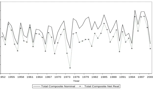
instruments. The tax rates by year used in our study are shown in Table 1 and they include taxes at the federal and state and local levels. We construct the return on residential housing using the data from the National Income and Product Accounts (NIPA) obtained from the Bureau of Economic Analysis (BEA) as well as the Flow of Funds Accounts (FFA) published by the Federal Reserve Board.3 The nominal and net real rates of return for the 1952-2000 period for assets in consideration are displayed in Figures 1 through 8. The real returns are not depicted since they closely approximate the net real rates as discussed below. The detailed description of the computations, data sources, and adjustments along with the total composite return data are presented in the appendices.

The overall composite return and the return for various groups of assets require weighting. The weight assigned to each asset in a group is its proportionate share in the total

value of assets held in the household sector as indicated in the previous section or as seen from following definition:4

∑

∑ ∑

∑

∑

r is the composite return; r_i is the total return on asset i; a_i is asset holdings, and w_i is

defined as the asset weight. We compute the composite rate of return using major asset classes in the representative household’s portfolio mentioned above. Since pension fund and life insurance reserves are a major part of household wealth, we include them in our household portfolio as well. Total household holdings for each asset are taken from the Flow of Funds Accounts.

The weighting scheme is based on a two-period moving average to slightly smooth out large atypical fluctuations in the weights.5 Thus,

⎟ ⎟ ⎟ ⎠ ⎞ ⎜ ⎜ ⎜ ⎝ ⎛ + =

∑

∑

w is the weight assigned to the ith asset at time t, and i t

a and ati−1 are the market values

of asset i at t and t−1. Figure 9 illustrates the total household portfolio composition. B. Discussion

Data presented in this section are computations on total returns. Total returns include returns on interest, dividends, net rental income from noncorporate and nongovernmental residential housing units, and capital gains. We have chosen to measure after-tax total returns

rather than after-tax interest rates because rational household behavior does not depend strictly

4 _{The weighting scheme arises from the portfolio analysis, and the weights are the market-based shares of each asset}

in the household portfolio.

on before-tax interest returns. Rational individuals hold portfolios of assets and pay attention to capital gains. Certainly, household behavior cannot logically focus on a particular interest rate such as the Treasury bill rate. To show why, define permanent consumption conventionally as the annuity value of wealth. If the Treasury bill rate (or the rate on any government risk-free bond) were the relevant rate of return, permanent consumption would be practically zero as the real after-tax return on Treasury bills over a long period of time is close to zero. Such a result is inconsistent with observed behavior.

We begin with eight variables consisting of returns on Treasury bills, Treasury notes, Treasury bonds, corporate bonds, municipal bonds, money, common stocks, and residential real estate. These variables are grouped to form nested collections. Specifically there is a group for government bonds, all bonds (including municipal and corporate bonds), all debt (including money), financial assets (including stocks), and all assets (including residential real estate). One can think of the lowest level collection consisting of government bonds as representing a

composite default risk-free rate and the highest level consisting of all financial assets and residential real estate as a proxy for the market rate of the CAPM.

Our focus in this section is primarily on the total composite return. We distinguish between nominal returns, real (after-inflation) returns defined in the manner of the Fisher

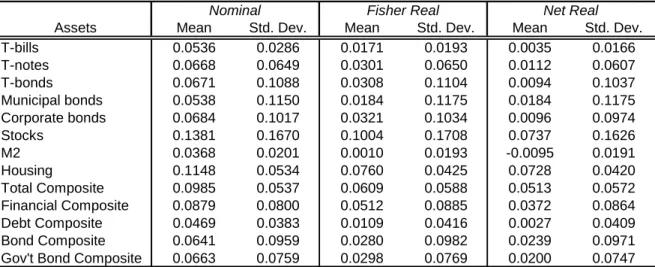
equation, and net real returns that take account of taxes. Table 2 presents descriptive statistics on the aggregate rate of return and its seven component assets as well as other composite groups for the period 1952-2000 in the United States. Figures 10 through 14 illustrate nominal and net real rates for our five composite measures. Some stark contrasts must be noted even if none will be particularly surprising upon reflection. First, note the difference between nominal or real returns to government securities, frequently used in research, and their net real returns. For Treasury

bills, specifically, the net real return over the period of forty-eight years was practically zero. The question asked much earlier, “Why is the risk-free rate so low?” becomes one of “Why is the risk-free rate almost zero?” If one were to think of the risk-free rate as a composite of

government debt, the net real rate of return was 2.0%.6 But there is an anomaly here. The

standard deviation for the composite of government bonds is rather high at 7.47%. If one accepts the notion that total returns are a more important variable in household decision making than interest returns, as we are asserting, this anomaly raises an interesting question: “Why would government bonds be called risk free if the definition of risk were the standard deviation?” This question arises because we have dropped the assumption of a fixed holding period. In contrast, the standard deviation of the net real interest rate (income return) for Treasury notes and bonds is about 2%. Ignoring capital gain component makes a huge impact on the standard deviation but not on the mean. The mean nominal capital gain return for Treasury notes and bonds is

practically zero since in the long run as bonds mature, capital gains and losses wash out.

In considering real rates of return, most analysts use the Fisher definition. Therefore, it is of interest to compare the data in the Fisher Real column with that in the Net Real column. One notes significant differences between the computations for Fisher real return and net real returns. It comes as no surprise that taxes make a difference. This difference made by taxes we call “level effects.” For single asset returns except housing, the level effects are notable. For instance, the net real Treasury bond rate is 0.94% vs. the Fisher real rate of 3.08%. The level effects between Fisher real and net real rates for two composite measures are shown in Figures 15 and 16. In Figure 15, the Fisher measure of the government bond composite is compared with the net

6 _{The reason why this composite figure is higher than the average of the values shown for government bond returns}

listed individually is that the weights in the composite are based on both household and pension fund holdings. The household portfolio contains Treasury notes and bonds both directly and indirectly and Treasury bills indirectly. Direct holdings are taxed at the average marginal tax rate on government interest. Indirect holdings through pension funds, etc. are not subject to tax, and as a result, the Fisher real, rather than net real, return is used.

real measure. The average difference is 0.98 percentage points. In Figure 16, the Fisher real composite for all assets is 6.09% vs. 5.13% for the net real composite. However, note strong correlations between the Fisher real and net real rate series. Differences in time variations, or time series effects, seem to be minimal.

For a different perspective, Table 3 presents a matrix showing how well the most

frequently used measures of returns correlate with the net real return on a composite of all assets (a more complete matrix is given in Appendix B), and Table 4 shows correlations for the net real composite measures. Assuming for the present that the total composite is the appropriate

measure for asset net returns, the data in Table 3 seem to indicate that neither of the commonly used risk-free rates is appropriate for empirical work. Both the Treasury bill and the Treasury bond rates are not well correlated with the total composite over the period of our study. Nor are they well correlated with the Fisher real total composite. However, Fisher real and net real composite measures are highly correlated. They are highly correlated because the standard deviations for the average marginal tax rates are much less than those for the rates of return. Note, too, that the correlations between stocks and both of the composite measures are high. However, as the next section on consumption will illustrate, a high correlation would not

necessarily indicate choosing the return on common stocks, if one needed a single asset measure, in lieu of the total composite return.

The high correlation between Fisher real and net real composite returns indicates that, in the absences of knowledge about taxes, Fisher real return is a suitable proxy measure of total returns if time series fluctuations are the most important to consider in econometric work. However, if level effects are important, Fisher real rate will not serve well. We conclude from this analysis that there is no adequate substitute for a total rate of return that does not take

account of taxes and is derived as a composite. In the next section we present results to indicate that an after-tax composite return has empirical as well as theoretical merit.

V. Estimation of Relative Risk Aversion and Intertemporal Elasticity of Substitution The usefulness of the total composite rate of return can be determined empirically. We investigate whether the use of the total composite is useful in estimating relative risk aversion (CRRA) and intertemporal elasticity of substitution (IES). We show that results derived by using the total composite are different from those obtained by using, for instance, the T-bill rate. In this section we test the validity of the consumption Euler equation using alternative measures of the rate of return. Previous attempts to validate the Euler approach to consumption theory with time series aggregate data generally have been unsuccessful. Lack of success could be due to one or more of four explanations: (1) the model is truly wrong, (2) specification of the utility function has been faulty, (3) aggregate consumption data are flawed, and (4) researchers have employed the wrong measure of the rate of return. Given our emphasis on the after-tax after-inflation total composite return, it seems reasonable to test its usefulness by applying it to the conventional approach in consumption economics. Accordingly, we focus on the fourth mentioned possible cause for rejection of the Euler approach. Our tests are conducted using an array of returns consisting of some singular measures and five composite measures. In our discussion, we first focus on the analysis of the total composite return, which represents a total household portfolio return, and the T-bill rate, which is a standard measure of the interest rate in consumption literature.

A. Major Previous Studies

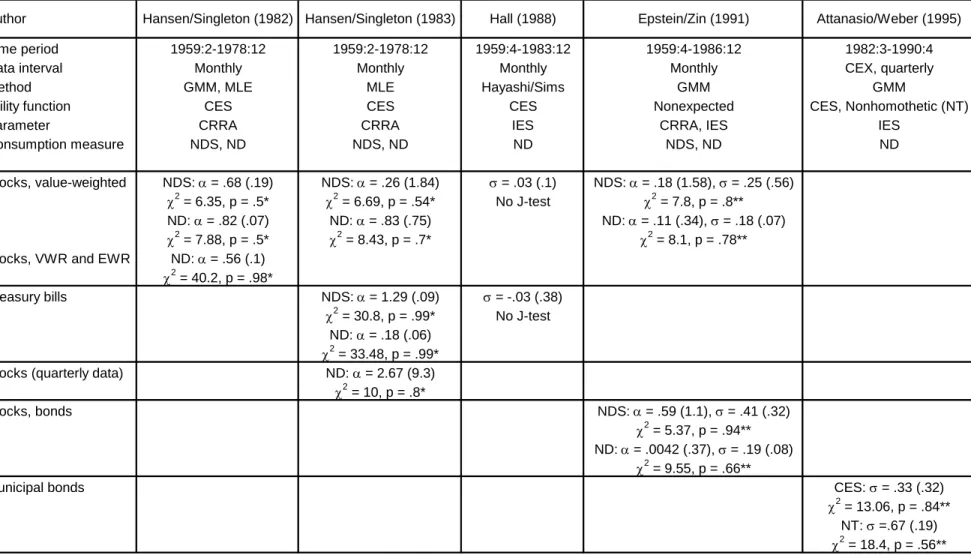
Table 5 gives the results of some of the estimates of relative risk aversion and

intertemporal elasticity of substitution from some well-known previous studies. We chose the specific estimates for the table because they were the ones most comparable with our estimates presented below. Using value-weighted and equally weighted NYSE stock returns as the measure of return and data on nondurables plus services (NDS) to represent consumption,

Hansen and Singleton (1982) estimated the parameters of the CES expected utility function using nonlinear version of the Euler equation. Their monthly data covered the period 1959:2-1978:12. They employed both instrumental variables and maximum likelihood approaches for estimation. When only the return on stocks was used and instrumental variables specified, the Hansen and Singleton’s estimate of relative risk aversion was statistically significant and there was no evidence against overidentifying restrictions of the model. However, their multiple return model that used both value- and equally weighted stock returns, rejected restrictions and provided evidence against the model.

Hansen and Singleton (1983) returned to the problem by formulating a restricted log-linear time series model to estimate the parameters of the CES utility function. They tested the model with value-weighted stock returns and the nominal risk-free Treasury bill rate using monthly data for the same period as previously. In the study they found statistically insignificant values for relative risk aversion using stock returns. Their estimate of relative risk aversion was statistically significant, but evidence against overidentifying restrictions was strong using the rate on Treasury bills as the measure of return. Hall (1988) estimated intertemporal elasticity of substitution with a log-linear model but rejected the Hansen-Singleton one-period lagged

S&P stock index returns. Hall found what he considered to be a reasonable range of values for IES, very close to zero. He did not test for overidentifying restrictions, however.

Epstein and Zin (1991) questioned the use of the expected utility model. In its place they substituted a more general nonexpected utility approach that permitted the disentangling of relative risk aversion and elasticity of substitution among other advantages. They chose four measures of consumption, three lag structures and two measures of returns (NYSE value

weighted stocks and stocks plus bonds), comprising a total of 24 models to be tested. They used monthly data for the time period used earlier by Hansen and Singleton and an extended time period, 1959:4-1986:12. Their generalized method of moments (GMM) estimates showed that the estimated parameter values were sensitive to model specification. Testing for overidentifying restrictions, the models were rejected in fourteen out of twenty-four tests.

Attanasio and Weber (1995) argued against the use of time series data in estimating Euler equations. They constructed panels from Consumer Expenditure Survey (CEX) data set for each year for 1982-1990. Using the yield on municipal bonds and specifying utility as CES, their estimate of IES was not statistically different from zero but there was no evidence against overidentifying restrictions. Switching to nonhomothetic utility, the authors obtained a statistically significant estimate of IES (0.67) with little evidence of overidentification.

B. Empirical Methodology

We conclude that the studies cited above find at best weak support for the CES model in time series tests and most of the estimates for IES are statistically insignificant using stock returns or the T-bill rate. We speculate that failure of the model has been due as much to misspecification of the rate of return variable as, perhaps, to misspecification of the utility function. In a representative agent and one asset world model, the relevant rate of return cannot

be that of a T-bill or stocks. The representative agent holds a portfolio of assets. We need to recognize that the return of concern is the return on the portfolio and not each individual return. Therefore, we test the conventional CES model while insisting that the representative consumer is also a CAPM-type investor, and that finance theory has a role to play in estimating parameters of an expected utility model.

Yet, a researcher must exercise some caution. Our task is not to see whether we can generate unambiguously “good” estimates of the parameters of a consumption Euler equation. Rather we only intend to investigate whether the use of the total composite net real rate as a measure of return yields different results than those obtained from single asset measures of return. Accordingly, we employ the conventional CES model used in early tests and substitute the composite return for the rate of return variables used in earlier studies. It is probable that using our total composite return with some other assumption about utility would produce better (worse) results; but experimenting with other utility functions is not our goal. Our experiments do not use any new technique, complicated utility functions or require panel data. Our estimated equations are the same as the relatively simple linear and nonlinear equations (derived from Euler equation (4)) that were standard in most of the tests of models undertaken earlier, namely:

(

)

(

)

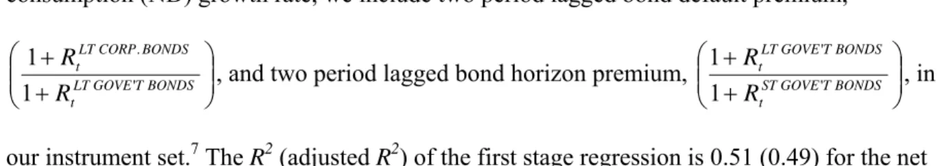
where σ and γ are the IES and CRRA, respectively. We use the GMM estimator of Hansen (1982) and perform our estimations in TSP. In addition to a constant and two, three, and four period lagged net real (or real if the real rate is used in estimations) T-bill rate and nondurable

consumption (ND) growth rate, we include two period lagged bond default premium, ⎟⎟ ⎠ ⎞ ⎜⎜ ⎝ ⎛ + + BONDS T GOVE LT t BONDS CORP LT t R R ' . 1 1

, and two period lagged bond horizon premium, _⎟⎟ ⎠ ⎞ ⎜⎜ ⎝ ⎛ + + BONDS T GOVE ST t BONDS T GOVE LT t R R ' ' 1 1 , in

our instrument set.7 The R2 (adjusted R2) of the first stage regression is 0.51 (0.49) for the net

real T-bill rate and 0.1 (0.06) for the total composite return. The instruments are lagged at least two periods due to the MA(1) component of the error term arising from aggregation (Hall 1988).

We estimate parameters in these equations using our quarterly data for the whole sample, 1952-2000. We also perform estimations for the time period selected by Hansen and Singleton (1983), Epstein and Zin (1991) (Hall’s 1988 time period plus three years), other periods, 1959-1996, 1965-2000, and 1979-2000, and a longer period, 1959-2000. Various time periods are used because we are interested in determining whether our results are independent of the periods selected for the experiments. We also utilize two measures of consumption, NDS for

nondurables and services and ND for nondurables taken from Table 7.1 (former Table 8.7) in the NIPA. In our discussion, we first focus on the analysis between the T-bill rate and the total composite return estimations. We also perform estimations using other single asset rates of return as well as several composite measures to represent the rate of return.

C. T-bill vs. Total Composite

Table 6 presents estimates for the net real T-bill rate and total composite return equations for both linear and nonlinear estimations as well as NDS and ND measures of consumption. First, with two measures of consumption and a linear estimation, for both returns the model is not rejected as indicated by the J-test of overidentifying restrictions while the IES parameters are estimated with precision. Using NDS, we note that the IES estimate is about 0.28 for the T-bill

7 _{We also used combinations of these instruments in addition to the stock return as well as nominal returns and the}

inflation rate in the instrument set for the T-bill and total composite estimations. The results do not change by any significant amount.

rate equation versus 0.15 for the total composite return equation. With ND, the IES estimate using the T-bill rate is slightly higher at 0.38 while the estimate using the total composite rises from 0.15 to 0.24. Intuitively, a 1% increase in the expected total composite rate increases the expected consumption growth rate by 0.24%.

However, for the nonlinear estimation, the J-test rejects the overidentifying restrictions for the model with the T-bill rate, unlike that with the total composite, at the 5% level for NDS and ND. The CRRA estimates for the total composite are substantially larger (2.91 vs. 1.16 for NDS and 2.55 vs. 0.82 for ND). In the table, we also present the corresponding IES estimates since in the CES utility model, the IES is an inverse of the CRRA (the standard errors are

computed using the delta method). Given this relationship and our estimates, we test whether this relationship is valid for both measures of return.8 The results are similar for NDS with p-values of 0.03 for both returns thus rejecting the hypothesis at the 5% level. For ND, the relationship holds for the total composite return at the 10% level (p-value of 0.14) but for the T-bill, it only holds at the 5% level (p-value of 0.07).

We also perform an empirical test of whether the total composite return has explanatory power in the linear model. We run the following regression:

(

)

and test whether δ =0. The results in Table 6 show that the hypothesis is rejected at the 5% level for both NDS and ND. Alternatively, equation (9) can be rewritten:

(

)

(

)

( )

(

)

The estimation results of equation (10) show that the coefficient on the T-bill rate is statistically insignificant while it is significant for the total composite as indicated by the estimate of δ . These results suggest that the total composite is more relevant than the T-bill in the household’s intertemporal problem.

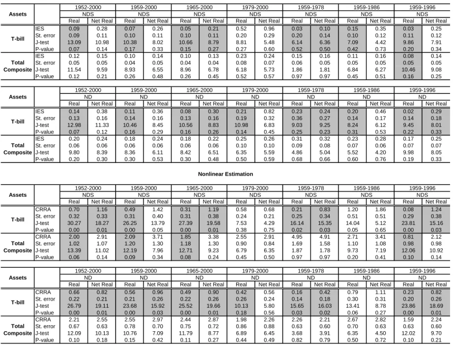
Table 7 presents the estimation results for real and net real rates and different sample periods. The shaded rows indicate that (i) the J-test values for overidentifying restrictions are not met at the 5% level, or (ii) given that the J-test does not reject the null of overidentifying

restrictions, the estimates for the parameters for relative risk aversion and intertemporal substitution are not significant at the 5% level. For linear estimations, we note that the IES estimates using the total composite return do not vary much from the 1952-2000 estimates. For the T-bill rate, for the 1959-1978 and 1965-2000 sample periods, the IES estimate is statistically insignificant, and for the 1979-2000 time period, the estimate is much larger. The results for nonlinear estimations also suggest that the IES estimates using the total composite return do not change much across sample periods. We also note that the J-test rejects the net real T-bill rate model in four (three) additional sample periods for ND (NDS).

Lastly, the issue of taxation seems to be much more important if using the T-bill rate than using the total composite return. This is not surprising as the fluctuations in the total composite return are much larger than the fluctuations in the tax rates with the correlation of the net real and real total composite rates of 0.99. For the T-bill rate, however, taxes seem to matter as

fluctuations in the rate of return are not as large relatively to the tax rates changes with the correlation of the net real and real T-bill rates of 0.94. The IES parameter using the net real total composite return is slightly higher and more precisely estimated than that using the real total composite rate. The difference is more pronounced for the T-bill return estimations. The IES

parameters are larger for the net real T-bill rate, for instance, 0.28 vs. 0.09 for the 1952-2000 period using NDS. In addition, the IES estimate using the net real T-bill rate is much more precisely estimated across different sample periods for both linear and nonlinear estimations.

In summary, taking into account different sample periods, NDS and ND consumption measures, and linear and nonlinear estimations, the total composite produces robust results in the Euler equation estimations. In addition, the test of the regression in equation (9) indicates that the total composite rate is more important in explaining the household’s consumption growth. The IES estimates are lower than those obtained using the T-bill rate and are in 0.15-0.3 range. However, we should note that in linear estimations, use of the T-bill rate also results in precisely estimated IES coefficients although the estimates are larger. Not surprisingly, a correlation coefficient between the T-bill rate and ND (NDS) consumption growth rate series is about 0.28 (0.23), which is slightly higher than that for the total composite, 0.2 (0.18).

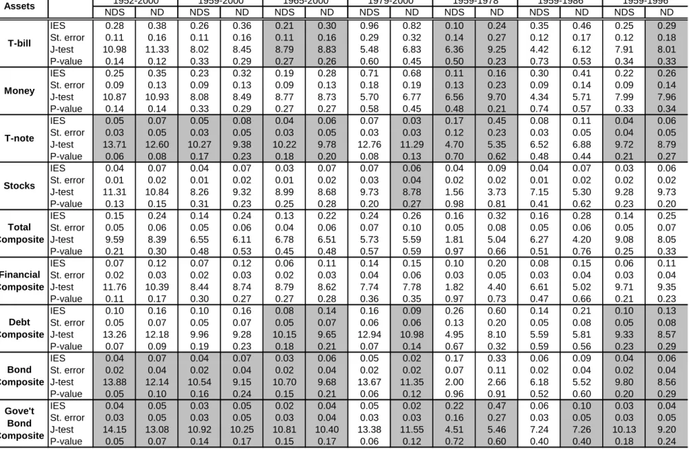
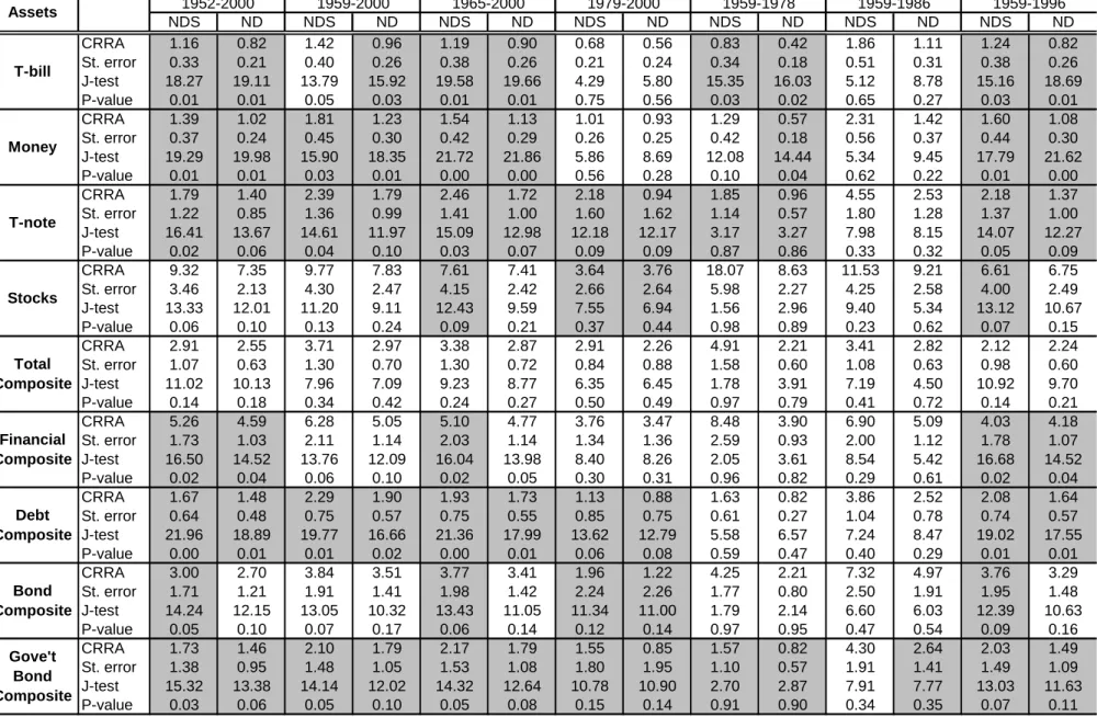
D. Other measures of return

Tables 8 and 9 present estimates for linear and nonlinear estimations for other measures of return. For linear estimations, the J-test does not reject the null of overidentifying restrictions at the 5% level for all measures of returns and consumption as well as time periods. However, for all return measures except for the total and financial composites, the IES parameter is imprecisely estimated for some time periods. Note that the IES estimate for the money return is quite similar to that of the T-bill rate, which is expected given that the M2 own rate follows closely the T-bill rate. The IES estimates using the T-note, bond and government bond composites are similar at about 0.05, but are imprecisely estimated. The estimate for the debt composite, whose main asset is money, is a little larger at 0.1 for NDS and 0.16 for ND for the 1952-2000 period. The use of the financial composite, whose main component is stocks, results

in a higher estimate of the IES (0.06-0.2) as compared to that for stocks (0.03-0.09). In general, the IES parameter estimates are lower than those for the total composite when using other asset measures except for money, which is comparable to the T-bill.

The nonlinear estimations suggest that in 9 out of 14 cases, the J-test rejects

overidentifying restrictions for the T-bill and money rates equations. Using Treasury notes, the model is not rejected except in 3 cases, but estimates of about 2 are statistically insignificant except for the 1959-1986 sample period. For the debt composite, the estimates are slightly larger (about 2) than for the money equation. Yet for the debt composite equation, the overidentifying restrictions are rejected in 8 out of 14 cases and the parameters are imprecisely estimated in 2 cases. Results derived by using the government bond composite produce mainly insignificant estimates although estimates are close to those for the T-notes. The use of the bond composite results in insignificant estimates in 5 cases while the CRRA estimates are a little larger than those for the total composite for some sample periods.

Stocks meet both tests except in 4 cases, but the estimates of CRRA for some time periods will appear to be too high. When the total composite is used as the rate of return, all tests are met and the coefficient of relative risk aversion falls within a range of 2.12-4.91 clustering around 2.5-3.5. By standards of the past, these estimates will seem reasonable to many

researchers. The financial composite, which comprises all assets except residential real estate, performs similar to stocks. However, the estimates for CRRA are quite larger (3.47-8.48) than the estimates for the total composite although lower than those for stocks (3.64-18.07). There is not much support in the literature for CRRA estimates above 5. The reason is that we do not observe insurance rates as high as one would expect to see if, in fact, CRRA for the

representative consumer fell within, for instance, the range of 5-10.9 Even CRRA in the range of 4-5 is considered to be very high. In contrast, the use of the total composite provides more reasonable estimates mostly in the range of about 2.5-3.5.

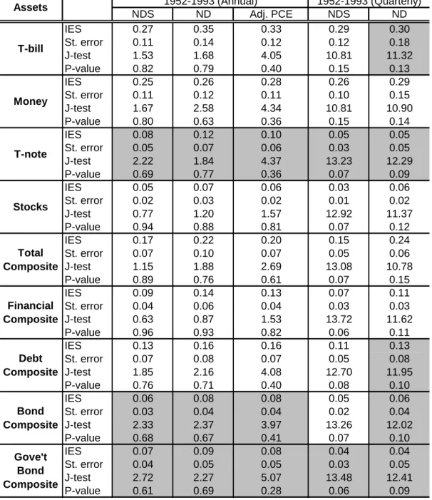
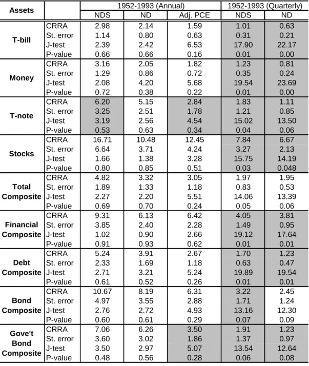
E. Alternative Measure of Consumption

Lastly, we use adjusted personal consumption expenditures (PCE) compiled by Slesnick (1998) and repeat the above exercise. These data account for service flows from durable goods and incorporate adjustments on expenditures by nonprofit institutions and insurance and medical care spending by households. The data are available annually for the 1952-1993 period. Our estimates are presented in Table 10 for the IES and Table 11 for the CRRA. Table 10 reveals that the IES estimates do not change much from those of ND and NDS consumption measures given the annual or quarterly 1952-1993 sample period. Thus the IES estimates are quite robust to data frequency. Moreover, the IES estimates with the adjusted PCE data are similar to those with NDS and ND. Note that the estimate for the total composite is 0.2 and is lower than that for the T-bill, 0.33. The nonlinear estimations suggest higher CRRA parameters for the annual data. The use of the adjusted PCE data results in the parameter estimates for the total composite of about 3 and for the T-bill of about 1.6, within the ranges obtained previously. As before but with a different consumption measure, the parameter estimates obtained using the total composite rate differ from those obtained using the T-bill rate.

VI. Concluding Remarks

We have constructed composite net real rates of return for five nested groups of assets:

thegovernment bonds, all bonds including municipal and corporate bonds, debt instruments

including money, financial assets including corporate ownership shares (stocks), and a representative portfolio of all major household assets including residential real estate. Each component return of each composite are computed as net real total returns. They include

periodic capital gains as well as income payments (interest and dividends) net of appropriate periodic tax rates and inflation. The components are value weighted to form composite rates of return.

Comparisons have been made between net real returns and Fisher real returns that do not

take account of taxes. Taxes are important for their level effects but not for time series effects.

Net real returns and Fisher real returns are highly correlated because tax rate changes from

period to period are small relatively to other changes. However, taxes claim on average over the past fifty years 30-40% of income due to interest and dividends and about 5% on capital gains. Capital gains and losses, both in stocks and bonds, are the main cause for the high volatility in component and composite returns.

We have attempted to answer the question, “Are composite returns, especially the total composite return, useful for consumption economics?” To answer this important question we have conducted an experiment using the household’s intertemporal problem. Noting that previous research to estimate parameters of consumption Euler equations (with CES utility and returns based on single assets) did not validate those models or produce precise parameters with aggregate time series data, we substituted the total composite return for single asset returns. The total composite return was more relevant to the intertemporal optimization than other composite measures and single asset returns. With linear and nonlinear estimations, different consumption measures, and various time periods, the use of the total composite return, the weighted-average portfolio return of a representative household, suggests that the IES is about 0.15-0.3 and the

CRRA is about 2.5-3.5. Our results thus show that the total composite return has a role to play in the household’s intertemporal consumption choice.

Ours will not be the last word on the usefulness of a macro-based measure of returns. Much work needs to be done. The idea behind our research seems reasonable; but to convince others of its usefulness requires better collection, processing, and understanding of data better than we can claim. Just as there is a large staff to compile national income accounts and prices, a relatively large staff will be needed to collect and process detailed information on rates of return. We have painted with a broad brush. A staff, perhaps, at the U. S. Commerce Department or Federal Reserve would include expertise in areas of data collection, financial accounting, and statistical analysis. Undoubtedly, such a staff would want to include additional categories of assets and study in more detail the special characteristics of them.

References

Attanasio, Orazio and Guglielmo Weber. “Is Consumption Growth Consistent with

Intertemporal Optimization? Evidence from the Consumer Expenditure Survey.” Journal of Political Economy v103, n6 (December 1995): 1121-1157.

Barro, Robert and Chaipat Sahasakul. “Measuring the Average Marginal Tax Rate from the Individual Income Tax.” Journal of Business v56 (October 1983): 419-452.

Brealey, Richard and Sabrina Kwan. “Personal Taxes and the Time Variation of Stock Returns – Evidence from the UK.” Journal of Banking & Finance v23 (1999): 1557-1577.

Cook, Timothy Q. and Patric H. Hendershott. “The Impact of Taxes, Risk and Relative Security Supplies on Interest Rate Differentials.” Journal of Finance v33, n4 (September 1978):

1173-1186.

Darby, Michael R. “The Financial and Tax Effects of Monetary Policy on Interest Rates.”

Economic Inquiry v13, n2 (June 1975): 266-76.

Epstein, Larry G. and Stanley E. Zin. “Substitution, Risk Aversion, and Temporal Behavior of Consumption and Asset Returns: an Empirical Analysis.” Journal of Political Economy v99, n2 (April 1991): 263-286.

Feldstein, Martin S. “Inflation, Income Taxes, and the Rate of Interest: A Theoretical Analysis.”

American Economic Review v66, n5 (December 1976): 809-20.

Feldstein, Martin, Jerry Green, and Eytan Sheshinski. “Inflation and Taxes in a Growing

Economy with Debt and Equity Finance.” Journal of Political Economy v86, n2 (1978):

S53-S70.

Feldstein, Martin S. and Lawrence Summers. “Inflation, Tax Rules, and the Long-Term Interest Rate.” Brookings Papers on Economic Activity v1 (1978): 61-99.

Fisher, Irving. Appreciation and Interest. Publications of the American Economic Association,

Third Series v11, n4, August 1896.

Hall, Robert E. “Intertemporal Substitution in Consumption.” Journal of Political Economy

v96, n2 (April 1988): 339-357.

Hansen, Lars P. “Large Sample Properties of Generalized Method of Moments Estimators.”

Econometrica v50, n4 (July 1982): 1029-1054.

Hansen, Lars. P. and Kenneth J. Singleton. “Generalized Instrumental Variables Estimation of Nonlinear Rational Expectations Models.” Econometrica v50, n5 (September 1982):

1269-1286.

Hansen, Lars. P. and Kenneth J. Singleton. “Stochastic Consumption, Risk Aversion, and the Temporal Behavior of Asset Returns.” Journal of Political Economy v91, n2 (April

1983): 249-265.

Hasanov, Fuad. “Measuring and Analyzing Returns on Residential Real Estate.” The University of Texas at Austin, working paper, 2003.

Hendershott, Patric H. and Joe Peek. “Treasury Bill Rates in the 1970s and 1980s.” Journal of Money, Credit, and Banking v24, n2 (May 1992): 195-214.

Ibbotson, Roger G. Stocks, Bonds, Bills, and Inflation, 1997 Yearbook. Chicago: R.G. Ibbotson

Associates, 1997.

Ibbotson, Roger G. Stocks, Bonds, Bills, and Inflation, 2001 Yearbook. Chicago: R.G. Ibbotson

Associates, 2001.

Ibbotson, Roger G., and Carol L. Fall. “The United States Market Wealth Portfolio.” The Journal of Portfolio Management (Fall 1979): 82-92.

Reform, the Cost of Capital, and US Economic Growth. Cambridge, MA: MIT Press,

2001.

Mankiw, Gregory N. “Consumer Spending and the After-Tax Real Interest Rate.” The Effects of Taxation on Capital Accumulation. Ed. Martin Feldstein. Chicago and London:

University of Chicago Press, 1987, 53-68.

Mishkin, Frederic S. “The Real Interest Rate: An Empirical Investigation.” Carnegie-Rochester Conference Series on Public Policy v15 (Autumn 1981): 151-200.

Mulligan, Casey B. “Capital, Interest, and Aggregate Intertemporal Substitution.” NBER working paper 9373, 2002.

Peek, Joe and James A. Wilcox. “The Degree of Fiscal Illusion in Interest Rates: Some Direct Estimates.” American Economic Review v74, n5 (December 1984): 1061-1066.

Peek, Joe and James A. Wilcox. “Tax Rates and Interest Rates on Tax-Exempt Securities.” New England Economic Review (January-February 1986): 29-41.

Roll, Richard. “A Critique of the Asset Pricing Theory's Tests: Part I: On Past and Potential Testability of the Theory.” Journal of Financial Economics v4, n2 (March 1977): 129-76.

Shiller, Robert J. “Can the Federal Reserve Control Real Interest Rates?” Rational Expectations and Economic Policy. Ed. Stanley Fischer. Cambridge, MA and Chicago: National

Bureau of Economic Research and University of Chicago Press, 1980.

Siegel, Laurence B. and David Montgomery. “Stocks, Bonds, and Bills after Taxes and Inflation.” The Journal of Portfolio Management v21, n2 (Winter 1995): 17-25.

Slesnick, Daniel T. “Are Our Data Relevant to the Theory? The Case of Aggregate

Consumption.” Journal of Business and Economic Statistics v16, n1 (January 1998):

Tanzi, Vito. “Inflation, Indexation and Interest Income Taxation.” Banca Nazionale del Lavoro Quarterly Review v116 (March 1976): 64-76.

Tobin, James. “Liquidity Preference as Behavior Towards Risk.” Review of Economic Studies,

v25, n2 (February 1958): 65-86.

United States. Board of Governors of the Federal Reserve System. “Flow of Funds Accounts of the United States.” 2003. Online. Internet. Jun. 2003. Available:

http://www.federalreserve.gov/releases/z1/Current/data.htm

United States. Board of Governors of the Federal Reserve System. “H.15 Selected Interest Rates.” 2001. Online. Internet. Jul. 2001. Available:

http://www.federalreserve.gov/releases/H15/data.htm

United States. Federal Reserve Bank of St. Louis. FRED Database. “M2 Own Rate.” 2001. Online. Internet. Jul. 2001. Available:

http://research.stlouisfed.org/fred2/series/M2OWN/24

United States. Department of Commerce. Bureau of Economic Analysis. “National Income and Product Accounts.” 2003. Online. Internet. Jun. 2003. Available:

http://www.bea.doc.gov/bea/dn/nipaweb/index.asp

United States. Department of Labor. Bureau of Labor Statistics. Selective Data Access Home Page: CPI. Online. Internet. Jul. 2001. Available: http://www.bls.gov/data/sa.htm United States. Department of Treasury. Treasury Bulletin, various years.

Table 1. Average Marginal Tax Rates on Household Income and Capital Gains, 1952-2000

Income from

Year Interest Corporate

Interest

Government Interest

Corporate

Dividends Capital Gains

Noncorporate Capital Gains 1952 0.3251 0.3182 0.2260 0.4862 0.0608 0.0406 1953 0.3093 0.3083 0.2153 0.4506 0.0563 0.0387 1954 0.2731 0.3182 0.1864 0.4411 0.0551 0.0341 1955 0.2740 0.2628 0.1941 0.4536 0.0567 0.0342 1956 0.2860 0.2276 0.2073 0.4680 0.0585 0.0357 1957 0.2820 0.1843 0.1548 0.4498 0.0562 0.0353 1958 0.2782 0.2361 0.2010 0.4473 0.0559 0.0348 1959 0.2809 0.2177 0.2113 0.4570 0.0571 0.0351 1960 0.2711 0.2123 0.2042 0.4435 0.0554 0.0339 1961 0.2713 0.2239 0.2035 0.4478 0.0560 0.0339 1962 0.2669 0.2191 0.2041 0.4382 0.0548 0.0334 1963 0.2878 0.2298 0.2248 0.4609 0.0576 0.0360 1964 0.2584 0.1991 0.2044 0.4230 0.0529 0.0323 1965 0.2329 0.1717 0.1884 0.3877 0.0485 0.0291 1966 0.2376 0.1752 0.1977 0.3929 0.0491 0.0297 1967 0.2464 0.1854 0.2030 0.4006 0.0501 0.0308 1968 0.2725 0.2082 0.2255 0.4318 0.0540 0.0341 1969 0.2843 0.2189 0.2419 0.4465 0.0558 0.0355 1970 0.2813 0.2243 0.2369 0.4151 0.0519 0.0352 1971 0.2718 0.2205 0.2280 0.4099 0.0512 0.0340 1972 0.2808 0.2292 0.2363 0.4183 0.0523 0.0351 1973 0.2911 0.2400 0.2507 0.4324 0.0541 0.0364 1974 0.3018 0.2525 0.2655 0.4405 0.0551 0.0377 1975 0.3035 0.2620 0.2641 0.4507 0.0563 0.0379 1976 0.3105 0.2729 0.2685 0.4610 0.0576 0.0388 1977 0.3157 0.2780 0.2761 0.4630 0.0579 0.0395 1978 0.3145 0.2780 0.2786 0.4603 0.0575 0.0393 1979 0.3292 0.2896 0.2964 0.4767 0.0477 0.0329 1980 0.3489 0.3061 0.3158 0.4883 0.0488 0.0349 1981 0.3578 0.3146 0.3255 0.4743 0.0474 0.0358 1982 0.3226 0.2814 0.2956 0.4093 0.0409 0.0323 1983 0.2977 0.2608 0.2730 0.3946 0.0395 0.0298 1984 0.2997 0.2654 0.2781 0.3923 0.0392 0.0300 1985 0.3010 0.2698 0.2801 0.3855 0.0385 0.0301 1986 0.2959 0.2612 0.2730 0.3944 0.0394 0.0296 1987 0.2800 0.2508 0.2604 0.3193 0.0798 0.0700 1988 0.2557 0.2305 0.2391 0.2842 0.0711 0.0639 1989 0.2625 0.2398 0.2458 0.2873 0.0718 0.0656 1990 0.2615 0.2401 0.2459 0.2856 0.0714 0.0654 1991 0.2619 0.2413 0.2441 0.2886 0.0721 0.0655 1992 0.2605 0.2394 0.2408 0.2885 0.0721 0.0651 1993 0.2827 0.2609 0.2599 0.3076 0.0769 0.0707 1994 0.2851 0.2653 0.2669 0.3082 0.0771 0.0713 1995 0.2913 0.2737 0.2739 0.3168 0.0792 0.0728 1996 0.2952 0.2802 0.2796 0.3199 0.0800 0.0738 1997 0.3007 0.2877 0.2847 0.3463 0.0866 0.0752 1998 0.2947 0.2840 0.2801 0.3193 0.0798 0.0737 1999 0.2964 0.2877 0.2833 0.3168 0.0792 0.0741 2000 0.2955 0.2887 0.2828 0.3159 0.0790 0.0739

Table 2. Descriptive Statistics on Composite and Component Returns (1952-2000)

Nominal Fisher Real Net Real

Assets Mean Std. Dev. Mean Std. Dev. Mean Std. Dev.

T-bills 0.0536 0.0286 0.0171 0.0193 0.0035 0.0166 T-notes 0.0668 0.0649 0.0301 0.0650 0.0112 0.0607 T-bonds 0.0671 0.1088 0.0308 0.1104 0.0094 0.1037 Municipal bonds 0.0538 0.1150 0.0184 0.1175 0.0184 0.1175 Corporate bonds 0.0684 0.1017 0.0321 0.1034 0.0096 0.0974 Stocks 0.1381 0.1670 0.1004 0.1708 0.0737 0.1626 M2 0.0368 0.0201 0.0010 0.0193 -0.0095 0.0191 Housing 0.1148 0.0534 0.0760 0.0425 0.0728 0.0420 Total Composite 0.0985 0.0537 0.0609 0.0588 0.0513 0.0572 Financial Composite 0.0879 0.0800 0.0512 0.0885 0.0372 0.0864 Debt Composite 0.0469 0.0383 0.0109 0.0416 0.0027 0.0409 Bond Composite 0.0641 0.0959 0.0280 0.0982 0.0239 0.0971

Gov't Bond Composite 0.0663 0.0759 0.0298 0.0769 0.0200 0.0747

Table 3. Correlation Matrix for Net Real Rates and Inflation (1952-2000)

T-Bill 1.000 T-Note 0.606 1.000 T-Bond 0.536 0.956 1.000 Municipals 0.530 0.903 0.889 1.000 Corp. Bonds 0.551 0.956 0.960 0.938 1.000 Stocks 0.382 0.275 0.303 0.347 0.392 1.000 Money 0.921 0.593 0.550 0.582 0.592 0.498 1.000 Housing 0.062 -0.007 0.046 0.080 0.015 0.092 0.002 1.000 Total Composite 0.505 0.412 0.436 0.481 0.506 0.905 0.578 0.360 1.000 Inflation -0.662 -0.396 -0.386 -0.419 -0.420 -0.470 -0.851 0.046 -0.486 1.000 Total Composite Inflation Corp.

Bonds Stocks Money Housing

T-Bill T-Note T-Bond Municipals

Table 4. Correlation Matrix for Net Real Composite Rates (1952-2000)

Total Financial Debt Bond Gove't Bond

Total Composite 1.0000

Financial Composite 0.9545 1.0000

Debt Composite 0.5706 0.6245 1.0000

Bond Composite 0.4883 0.5324 0.9553 1.0000

Table 5. Estimates of CRRA and IES from Previous Studies

Time period 1959:2-1978:12 1959:2-1978:12 1959:4-1983:12 1959:4-1986:12 1982:3-1990:4

Data interval Monthly Monthly Monthly Monthly CEX, quarterly

Method GMM, MLE MLE Hayashi/Sims GMM GMM

Utility function CES CES CES Nonexpected CES, Nonhomothetic (NT)

Parameter CRRA CRRA IES CRRA, IES IES

Consumption measure NDS, ND NDS, ND ND NDS, ND ND Stocks, value-weighted NDS: α = .68 (.19) NDS: α= .26 (1.84) σ= .03 (.1) NDS: α= .18 (1.58), σ= .25 (.56) χ2 = 6.35, p = .5* χ2= 6.69, p = .54* No J-test χ2= 7.8, p = .8** ND: α = .82 (.07) ND: α= .83 (.75) ND: α= .11 (.34), σ= .18 (.07) χ2 = 7.88, p = .5* χ2= 8.43, p = .7* χ2= 8.1, p = .78** Stocks, VWR and EWR ND: α = .56 (.1)

χ2 = 40.2, p = .98* Treasury bills NDS: α= 1.29 (.09) σ= -.03 (.38) χ2 = 30.8, p = .99* No J-test ND: α= .18 (.06) χ2 = 33.48, p = .99* Stocks (quarterly data) ND: α= 2.67 (9.3)

χ2 = 10, p = .8* Stocks, bonds NDS: α= .59 (1.1), σ= .41 (.32) χ2 = 5.37, p = .94** ND: α= .0042 (.37), σ= .19 (.08) χ2 = 9.55, p = .66**

Municipal bonds CES: σ= .33 (.32)

χ2

= 13.06, p = .84** NT: σ=.67 (.19) χ2

= 18.4, p = .56**

Standard errors for parameter estimates are in parentheses; p indicates p-values. * Reject null if P > .95; ** Reject null if P < .05.

VWR = value-weighted return; EWR = equally weighted return.

Specific tests in papers reviewed were selected for comparability with tests made in this study.

Epstein/Zin (1991) Attanasio/Weber (1995) Author Hansen/Singleton (1982) Hansen/Singleton (1983) Hall (1988)

Table 6. T-bill Rate vs. Total Composite Return (1952:I-2000:IV) Parameter 0.28 0.15 1.16 2.91 0.86 0.34 St. error 0.11 0.05 0.33 1.07 0.25 0.13 J-test 10.98 9.59 18.27 11.02 18.27 11.02 P-value 0.14 0.21 0.01 0.14 0.01 0.14 Statistic -2.11 -2.21 P-value 0.03 0.03 σ 0.104 P-value 0.361 δ -0.170 P-value 0.028 Parameter 0.38 0.24 0.82 2.55 1.22 0.39 St. error 0.16 0.06 0.21 0.63 0.32 0.10 J-test 11.33 8.39 19.11 10.13 19.11 10.13 P-value 0.12 0.30 0.01 0.18 0.01 0.18 Statistic -1.79 -1.60 P-value 0.07 0.11 σ 0.068 P-value 0.709 δ -0.334 P-value 0.003 Equation (9) Test Equation (9) Test

CRRA Corresponding IES

T-bill Total Composite T-bill Total Composite Test for IES=1/CRRA Test for IES=1/CRRA Linear Nonlinear NDS ND Nonlinear T-bill Total Composite IES

Table 7. T-bill Rate vs. Total Composite Return (linear and nonlinear estimations)

Linear Estimation

1952-2000 1959-2000 1965-2000 1979-2000 1959-1978 1959-1986 1959-1996

Assets NDS NDS NDS NDS NDS NDS NDS

Real Net Real Real Net Real Real Net Real Real Net Real Real Net Real Real Net Real Real Net Real

IES 0.09 0.28 0.07 0.26 0.05 0.21 0.52 0.96 0.03 0.10 0.15 0.35 0.03 0.25 St. error 0.09 0.11 0.10 0.11 0.10 0.11 0.20 0.29 0.20 0.14 0.10 0.12 0.11 0.12 J-test 13.09 10.98 10.38 8.02 10.66 8.79 8.81 5.48 6.14 6.36 7.09 4.42 9.86 7.91 P-value 0.07 0.14 0.17 0.33 0.15 0.27 0.27 0.60 0.52 0.50 0.42 0.73 0.20 0.34 IES 0.12 0.15 0.10 0.14 0.10 0.13 0.23 0.24 0.15 0.16 0.11 0.16 0.08 0.14 St. error 0.05 0.05 0.04 0.05 0.04 0.04 0.08 0.07 0.06 0.05 0.05 0.05 0.05 0.05 J-test 11.54 9.59 8.93 6.55 8.96 6.78 6.18 5.73 1.86 1.81 6.84 6.27 10.46 9.08 P-value 0.12 0.21 0.26 0.48 0.26 0.45 0.52 0.57 0.97 0.97 0.45 0.51 0.16 0.25 1952-2000 1959-2000 1965-2000 1979-2000 1959-1978 1959-1986 1959-1996 Assets ND ND ND ND ND ND ND

Real Net Real Real Net Real Real Net Real Real Net Real Real Net Real Real Net Real Real Net Real

IES 0.14 0.38 0.11 0.36 0.08 0.30 0.21 0.82 0.23 0.24 0.20 0.46 0.02 0.29 St. error 0.13 0.16 0.14 0.16 0.13 0.16 0.19 0.32 0.36 0.27 0.14 0.17 0.14 0.18 J-test 12.98 11.33 10.46 8.45 10.56 8.83 10.98 6.83 9.03 9.25 8.24 6.12 9.45 8.01 P-value 0.07 0.12 0.16 0.29 0.16 0.26 0.14 0.45 0.25 0.23 0.31 0.53 0.22 0.33 IES 0.20 0.24 0.18 0.24 0.18 0.22 0.25 0.26 0.31 0.32 0.23 0.28 0.17 0.25 St. error 0.06 0.06 0.06 0.06 0.06 0.06 0.10 0.10 0.09 0.08 0.07 0.06 0.07 0.07 J-test 9.80 8.39 8.36 6.11 8.42 6.51 6.35 5.59 4.86 5.04 5.52 4.20 9.98 8.05 P-value 0.20 0.30 0.30 0.53 0.30 0.48 0.50 0.59 0.68 0.66 0.60 0.76 0.19 0.33 Nonlinear Estimation 1952-2000 1959-2000 1965-2000 1979-2000 1959-1978 1959-1986 1959-1996 Assets NDS NDS NDS NDS NDS NDS NDS

Real Net Real Real Net Real Real Net Real Real Net Real Real Net Real Real Net Real Real Net Real

CRRA 0.70 1.16 0.49 1.42 0.31 1.19 0.58 0.68 0.21 0.83 1.20 1.86 0.08 1.24 St. error 0.32 0.33 0.31 0.40 0.31 0.38 0.24 0.21 0.25 0.34 0.51 0.51 0.29 0.38 J-test 30.27 18.27 26.25 13.79 27.39 19.58 7.53 4.29 16.14 15.35 14.04 5.12 23.81 15.16 P-value 0.00 0.01 0.00 0.05 0.00 0.01 0.38 0.75 0.02 0.03 0.05 0.65 0.00 0.03 CRRA 2.00 2.91 2.09 3.71 1.85 3.38 2.55 2.91 4.95 4.91 2.71 3.41 0.81 2.12 St. error 1.02 1.07 1.20 1.30 1.18 1.30 0.90 0.84 1.69 1.58 1.10 1.08 0.98 0.98 J-test 13.39 11.02 12.19 7.96 12.71 9.23 6.79 6.35 1.87 1.78 9.73 7.19 12.06 10.92 P-value 0.06 0.14 0.09 0.34 0.08 0.24 0.45 0.50 0.97 0.97 0.20 0.41 0.10 0.14 1952-2000 1959-2000 1965-2000 1979-2000 1959-1978 1959-1986 1959-1996 Assets ND ND ND ND ND ND ND

Real Net Real Real Net Real Real Net Real Real Net Real Real Net Real Real Net Real Real Net Real

CRRA 0.66 0.82 0.56 0.96 0.49 0.90 0.42 0.56 0.16 0.42 0.79 1.11 0.23 0.82 St. error 0.22 0.21 0.21 0.26 0.22 0.26 0.26 0.24 0.14 0.18 0.30 0.31 0.20 0.26 J-test 26.79 19.11 23.68 15.92 25.52 19.66 10.13 5.80 15.65 16.03 13.41 8.78 23.86 18.69 P-value 0.00 0.01 0.00 0.03 0.00 0.01 0.18 0.56 0.03 0.02 0.06 0.27 0.00 0.01 CRRA 2.21 2.55 2.55 2.97 2.44 2.87 1.98 2.26 2.26 2.21 2.67 2.82 1.59 2.24 St. error 0.67 0.63 0.78 0.70 0.75 0.72 0.86 0.88 0.63 0.60 0.70 0.63 0.63 0.60 J-test 12.09 10.13 10.76 7.09 11.79 8.77 6.89 6.45 3.68 3.91 6.35 4.50 12.02 9.70 P-value 0.10 0.18 0.15 0.42 0.11 0.27 0.44 0.49 0.82 0.79 0.50 0.72 0.10 0.21 T-bill Total Composite T-bill Total Composite T-bill Total Composite T-bill Total Composite

Table 8. Estimates of the IES (linear estimation, net real rates) 1952-2000 1959-2000 1965-2000 1979-2000 1959-1978 1959-1986 1959-1996 NDS ND NDS ND NDS ND NDS ND NDS ND NDS ND NDS ND IES 0.28 0.38 0.26 0.36 0.21 0.30 0.96 0.82 0.10 0.24 0.35 0.46 0.25 0.29 St. error 0.11 0.16 0.11 0.16 0.11 0.16 0.29 0.32 0.14 0.27 0.12 0.17 0.12 0.18 J-test 10.98 11.33 8.02 8.45 8.79 8.83 5.48 6.83 6.36 9.25 4.42 6.12 7.91 8.01 P-value 0.14 0.12 0.33 0.29 0.27 0.26 0.60 0.45 0.50 0.23 0.73 0.53 0.34 0.33 IES 0.25 0.35 0.23 0.32 0.19 0.28 0.71 0.68 0.11 0.16 0.30 0.41 0.22 0.26 St. error 0.09 0.13 0.09 0.13 0.09 0.13 0.18 0.19 0.13 0.23 0.09 0.14 0.09 0.14 J-test 10.87 10.93 8.08 8.49 8.77 8.73 5.70 6.77 6.56 9.70 4.34 5.71 7.99 7.96 P-value 0.14 0.14 0.33 0.29 0.27 0.27 0.58 0.45 0.48 0.21 0.74 0.57 0.33 0.34 IES 0.05 0.07 0.05 0.08 0.04 0.06 0.07 0.03 0.17 0.45 0.08 0.11 0.04 0.06 St. error 0.03 0.05 0.03 0.05 0.03 0.05 0.03 0.03 0.12 0.23 0.03 0.05 0.04 0.05 J-test 13.71 12.60 10.27 9.38 10.22 9.78 12.76 11.29 4.70 5.35 6.52 6.88 9.72 8.79 P-value 0.06 0.08 0.17 0.23 0.18 0.20 0.08 0.13 0.70 0.62 0.48 0.44 0.21 0.27 IES 0.04 0.07 0.04 0.07 0.03 0.07 0.07 0.06 0.04 0.09 0.04 0.07 0.03 0.06 St. error 0.01 0.02 0.01 0.02 0.01 0.02 0.03 0.04 0.02 0.02 0.01 0.02 0.02 0.02 J-test 11.31 10.84 8.26 9.32 8.99 8.68 9.73 8.78 1.56 3.73 7.15 5.30 9.28 9.73 P-value 0.13 0.15 0.31 0.23 0.25 0.28 0.20 0.27 0.98 0.81 0.41 0.62 0.23 0.20 IES 0.15 0.24 0.14 0.24 0.13 0.22 0.24 0.26 0.16 0.32 0.16 0.28 0.14 0.25 St. error 0.05 0.06 0.05 0.06 0.04 0.06 0.07 0.10 0.05 0.08 0.05 0.06 0.05 0.07 J-test 9.59 8.39 6.55 6.11 6.78 6.51 5.73 5.59 1.81 5.04 6.27 4.20 9.08 8.05 P-value 0.21 0.30 0.48 0.53 0.45 0.48 0.57 0.59 0.97 0.66 0.51 0.76 0.25 0.33 IES 0.07 0.12 0.07 0.12 0.06 0.11 0.14 0.15 0.10 0.20 0.08 0.15 0.06 0.11 St. error 0.02 0.03 0.02 0.03 0.02 0.03 0.04 0.06 0.03 0.05 0.03 0.04 0.03 0.04 J-test 11.76 10.39 8.44 8.74 8.79 8.62 7.74 7.78 1.82 4.40 6.61 5.02 9.71 9.35 P-value 0.11 0.17 0.30 0.27 0.27 0.28 0.36 0.35 0.97 0.73 0.47 0.66 0.21 0.23 IES 0.10 0.16 0.10 0.16 0.08 0.14 0.16 0.09 0.26 0.60 0.14 0.21 0.10 0.13 St. error 0.05 0.07 0.05 0.07 0.05 0.07 0.06 0.06 0.13 0.20 0.05 0.08 0.05 0.08 J-test 13.26 12.18 9.96 9.28 10.15 9.65 12.94 10.98 4.95 8.10 5.59 5.81 9.33 8.57 P-value 0.07 0.09 0.19 0.23 0.18 0.21 0.07 0.14 0.67 0.32 0.59 0.56 0.23 0.29 IES 0.04 0.07 0.04 0.07 0.03 0.06 0.05 0.02 0.17 0.33 0.06 0.09 0.04 0.06 St. error 0.02 0.04 0.02 0.04 0.02 0.04 0.02 0.02 0.07 0.11 0.02 0.04 0.02 0.04 J-test 13.88 12.14 10.54 9.15 10.70 9.68 13.67 11.35 2.00 2.66 6.18 5.52 9.80 8.56 P-value 0.05 0.10 0.16 0.24 0.15 0.21 0.06 0.12 0.96 0.91 0.52 0.60 0.20 0.29 IES 0.04 0.05 0.03 0.05 0.02 0.04 0.05 0.02 0.22 0.47 0.06 0.10 0.03 0.04 St. error 0.03 0.05 0.03 0.05 0.03 0.04 0.03 0.03 0.16 0.27 0.03 0.05 0.03 0.05 J-test 14.15 13.08 10.92 10.25 10.81 10.40 13.38 11.55 4.51 5.46 7.24 7.26 10.13 9.20 P-value 0.05 0.07 0.14 0.17 0.15 0.17 0.06 0.12 0.72 0.60 0.40 0.40 0.18 0.24 Assets T-bill Money T-note Stocks Gove't Bond Composite Total Composite Financial Composite Debt Composite Bond Composite

Table 9. Estimates of the CRRA (nonlinear estimation, net real rates) 1952-2000 1959-2000 1965-2000 1979-2000 1959-1978 1959-1986 1959-1996 NDS ND NDS ND NDS ND NDS ND NDS ND NDS ND NDS ND CRRA 1.16 0.82 1.42 0.96 1.19 0.90 0.68 0.56 0.83 0.42 1.86 1.11 1.24 0.82 St. error 0.33 0.21 0.40 0.26 0.38 0.26 0.21 0.24 0.34 0.18 0.51 0.31 0.38 0.26 J-test 18.27 19.11 13.79 15.92 19.58 19.66 4.29 5.80 15.35 16.03 5.12 8.78 15.16 18.69 P-value 0.01 0.01 0.05 0.03 0.01 0.01 0.75 0.56 0.03 0.02 0.65 0.27 0.03 0.01 CRRA 1.39 1.02 1.81 1.23 1.54 1.13 1.01 0.93 1.29 0.57 2.31 1.42 1.60 1.08 St. error 0.37 0.24 0.45 0.30 0.42 0.29 0.26 0.25 0.42 0.18 0.56 0.37 0.44 0.30 J-test 19.29 19.98 15.90 18.35 21.72 21.86 5.86 8.69 12.08 14.44 5.34 9.45 17.79 21.62 P-value 0.01 0.01 0.03 0.01 0.00 0.00 0.56 0.28 0.10 0.04 0.62 0.22 0.01 0.00 CRRA 1.79 1.40 2.39 1.79 2.46 1.72 2.18 0.94 1.85 0.96 4.55 2.53 2.18 1.37 St. error 1.22 0.85 1.36 0.99 1.41 1.00 1.60 1.62 1.14 0.57 1.80 1.28 1.37 1.00 J-test 16.41 13.67 14.61 11.97 15.09 12.98 12.18 12.17 3.17 3.27 7.98 8.15 14.07 12.27 P-value 0.02 0.06 0.04 0.10 0.03 0.07 0.09 0.09 0.87 0.86 0.33 0.32 0.05 0.09 CRRA 9.32 7.35 9.77 7.83 7.61 7.41 3.64 3.76 18.07 8.63 11.53 9.21 6.61 6.75 St. error 3.46 2.13 4.30 2.47 4.15 2.42 2.66 2.64 5.98 2.27 4.25 2.58 4.00 2.49 J-test 13.33 12.01 11.20 9.11 12.43 9.59 7.55 6.94 1.56 2.96 9.40 5.34 13.12 10.67 P-value 0.06 0.10 0.13 0.24 0.09 0.21 0.37 0.44 0.98 0.89 0.23 0.62 0.07 0.15 CRRA 2.91 2.55 3.71 2.97 3.38 2.87 2.91 2.26 4.91 2.21 3.41 2.82 2.12 2.24 St. error 1.07 0.63 1.30 0.70 1.30 0.72 0.84 0.88 1.58 0.60 1.08 0.63 0.98 0.60 J-test 11.02 10.13 7.96 7.09 9.23 8.77 6.35 6.45 1.78 3.91 7.19 4.50 10.92 9.70 P-value 0.14 0.18 0.34 0.42 0.24 0.27 0.50 0.49 0.97 0.79 0.41 0.72 0.14 0.21 CRRA 5.26 4.59 6.28 5.05 5.10 4.77 3.76 3.47 8.48 3.90 6.90 5.09 4.03 4.18 St. error 1.73 1.03 2.11 1.14 2.03 1.14 1.34 1.36 2.59 0.93 2.00 1.12 1.78 1.07 J-test 16.50 14.52 13.76 12.09 16.04 13.98 8.40 8.26 2.05 3.61 8.54 5.42 16.68 14.52 P-value 0.02 0.04 0.06 0.10 0.02 0.05 0.30 0.31 0.96 0.82 0.29 0.61 0.02 0.04 CRRA 1.67 1.48 2.29 1.90 1.93 1.73 1.13 0.88 1.63 0.82 3.86 2.52 2.08 1.64 St. error 0.64 0.48 0.75 0.57 0.75 0.55 0.85 0.75 0.61 0.27 1.04 0.78 0.74 0.57 J-test 21.96 18.89 19.77 16.66 21.36 17.99 13.62 12.79 5.58 6.57 7.24 8.47 19.02 17.55 P-value 0.00 0.01 0.01 0.02 0.00 0.01 0.06 0.08 0.59 0.47 0.40 0.29 0.01 0.01 CRRA 3.00 2.70 3.84 3.51 3.77 3.41 1.96 1.22 4.25 2.21 7.32 4.97 3.76 3.29 St. error 1.71 1.21 1.91 1.41 1.98 1.42 2.24 2.26 1.77 0.80 2.50 1.91 1.95 1.48 J-test 14.24 12.15 13.05 10.32 13.43 11.05 11.34 11.00 1.79 2.14 6.60 6.03 12.39 10.63 P-value 0.05 0.10 0.07 0.17 0.06 0.14 0.12 0.14 0.97 0.95 0.47 0.54 0.09 0.16 CRRA 1.73 1.46 2.10 1.79 2.17 1.79 1.55 0.85 1.57 0.82 4.30 2.64 2.03 1.49 St. error 1.38 0.95 1.48 1.05 1.53 1.08 1.80 1.95 1.10 0.57 1.91 1.41 1.49 1.09 J-test 15.32 13.38 14.14 12.02 14.32 12.64 10.78 10.90 2.70 2.87 7.91 7.77 13.03 11.63 P-value 0.03 0.06 0.05 0.10 0.05 0.08 0.15 0.14 0.91 0.90 0.34 0.35 0.07 0.11 Assets Gove't Bond Composite Total Composite Financial Composite Debt Composite Bond Composite T-bill Money T-note Stocks

Table 10. Estimates of the IES (linear estimation, adjusted PCE, net real rates) 1952-1993 (Annual) 1952-1993 (Quarterly) NDS ND Adj. PCE NDS ND IES 0.27 0.35 0.33 0.29 0.30 St. error 0.11 0.14 0.12 0.12 0.18 J-test 1.53 1.68 4.05 10.81 11.32 P-value 0.82 0.79 0.40 0.15 0.13 IES 0.25 0.26 0.28 0.26 0.29 St. error 0.11 0.12 0.11 0.10 0.15 J-test 1.67 2.58 4.34 10.81 10.90 P-value 0.80 0.63 0.36 0.15 0.14 IES 0.08 0.12 0.10 0.05 0.05 St. error 0.05 0.07 0.06 0.03 0.05 J-test 2.22 1.84 4.37 13.23 12.29 P-value 0.69 0.77 0.36 0.07 0.09 IES 0.05 0.07 0.06 0.03 0.06 St. error 0.02 0.03 0.02 0.01 0.02 J-test 0.77 1.20 1.57 12.92 11.37 P-value 0.94 0.88 0.81 0.07 0.12 IES 0.17 0.22 0.20 0.15 0.24 St. error 0.07 0.10 0.07 0.05 0.06 J-test 1.15 1.88 2.69 13.08 10.78 P-value 0.89 0.76 0.61 0.07 0.15 IES 0.09 0.14 0.13 0.07 0.11 St. error 0.04 0.06 0.04 0.03 0.03 J-test 0.63 0.87 1.53 13.72 11.62 P-value 0.96 0.93 0.82 0.06 0.11 IES 0.13 0.16 0.16 0.11 0.13 St. error 0.07 0.08 0.07 0.05 0.08 J-test 1.85 2.16 4.08 12.70 11.95 P-value 0.76 0.71 0.40 0.08 0.10 IES 0.06 0.08 0.08 0.05 0.06 St. error 0.03 0.04 0.04 0.02 0.04 J-test 2.33 2.37 3.97 13.26 12.02 P-value 0.68 0.67 0.41 0.07 0.10 IES 0.07 0.09 0.08 0.04 0.04 St. error 0.04 0.05 0.05 0.03 0.05 J-test 2.72 2.27 5.07 13.48 12.41 Assets T-bill Money T-note Stocks Gove't Bond Total Composite Financial Composite Debt Composite Bond Composite