Variability and Uncertainty in Risk Estimation
for Brownfields Redevelopment
Arne Edward Olsen
Thesis Submitted to the Faculty of the Virginia Polytechnic Institute and State University in partial fulfillment of the requirements for the degree of
MASTER OF SCIENCE In
Environmental Science and Engineering Approved:
Dr. Naraine Persaud, Chair
Dr. Matthew Eick
Dr. William Moore
Sanjay V. Thirunagari
Keywords: Brownfields, Risk, Deterministic, Probabilistic
July 25, 2000 Blacksburg, Virginia
Variability and Uncertainty in Risk Estimation
for Brownfields Redevelopment
Arne E. Olsen Abstract
Various methods can be used to estimate the human health risk associated with exposure to contaminants at brownfields facilities. The deterministic method has been the standard practice, but the use of probabilistic methods is increasing. Contaminant data for non-carcinogens and non-carcinogens from 21 brownfields sites in Pennsylvania were collected and compiled. These were used to evaluate the performance of the deterministic and several probabilistic methods for assessing exposure and risk in relation to variability and uncertainty in the data set and input parameters. The probabilistic methods were based (a) entirely on Monte Carlo simulated input parameter distribution functions, (b) on a combination of some of these functions and fixed parameter values, or (c) on a parameter distribution function. These methods were used to generate contaminant intake doses, defined as the 90th, 95th, or 99.9th percentile of their estimated output distribution, for the principal human exposure routes. These values were then compared with the
corresponding point values estimated by the deterministic method. For all exposure routes the probabilistic intake dose estimates, taken as the 90th and 95th percentiles of the output distribution, were not markedly different from the deterministic values or from each other. The opposite was generally the case for the estimates at the 99.9th cutoff percentile, especially for the Monte Carlo-based methods. Increasing standard deviation of the input contaminant concentration tended to produce higher intake dose estimates for all estimation methods. In pairwise comparisons with the deterministic estimates, this trend differed significantly only for the probabilistic intake doses estimated as the 99.9th
percentile of the output distribution. Taken together, these results did not indicate clear and definitive advantages in using probabilistic methods over the deterministic method for exposure and risk assessment for brownfields redevelopment. They supported using the tired system for environmental risk assessment at any particular brownfields facility.
ACKNOWLEDGEMENTS
I would like to express my gratitude to Dr. Naraine Persaud for his guidance and direction to successfully complete this phase of my planned sojourn in graduate school. I would also like to thank Dr. Matthew Eick, Dr. William Moore, and Sanjay Thirunagari for the advice and support they have provided throughout this course of study. The Graduate Student Association award of funds to purchase the @Risk software package is very much appreciated. Lastly, I would like to thank my parents, Arne and Becky Olsen, for their support and encouragement during my graduate studies.
TABLE OF CONTENTS
Abstract i
ACKNOWLEDGEMENTS iii
TABLE OF CONTENTS iv
LIST OF TABLES v
LIST OF FIGURES viii
INTRODUCTION 1
LITERATURE REVIEW 6
2.1 Brownfields 6
2.2 Risk Assessment Methodology 9
2.2.1 Basic Concepts 9
2.2.2 Variability and Uncertainty in Risk Estimation 18
2.2.3 Deterministic Risk Assessment 20
2.2.4 Probabilistic Risk Assessment 23
MATERIALS AND METHODS 33
3.1 Brownfields Sites and Contaminant Data 33
3.2 Deterministic Risk Estimates 41
3.3 Probabilistic Risk Estimates 43
3.4 Statistical Analysis 46
RESULTS AND DISCUSSION 50
SUMMARY AND CONCLUSIONS 75
References 79
APPENDIX
Contaminant concentrations, their descriptive statistics and Land’s UCL95,
calculated mass transfer parameters, and @Risk best fits for soil, air, and
groundwater concentration distributions. 85
LIST OF TABLES
Table 1. Twenty-one sites taken from Pennsylvania's Land Recycling Program
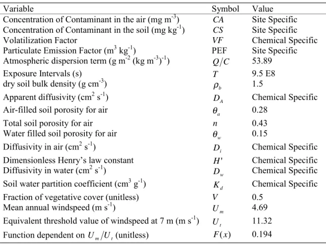
list of completed brownfields...34 Table 2. Parameter values for the intergerated soil to air emission and
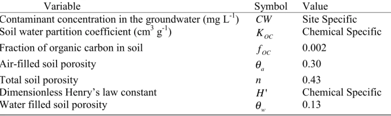
dispersion models...39 Table 3 . Parameter values for estimating groundwater concentraiton from
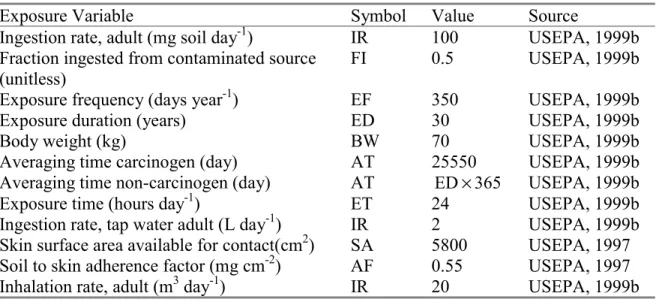
soil concentration ...40 Table 4. Values of exposure factors for the deterministic and Monte
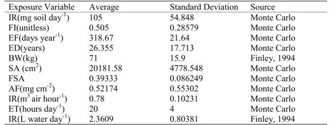
Carlo/deterministic analyses ...42 Table 5. Recommended density distributions and @ Risk 4.0 function
parameters (in parenthesis) for each exposure variable in the Monte Carlo
and Monte Carlo/deterministic analysis...44 Table 6. Mean and standard deviation of exposure variables used for the
two-point-based risk estimation method ...45 Table 7. Contaminant/site combinations and exposure routes for which intake
dose for non-carcinogens were estimated ...47 Table 8. Contaminant/site combinations and exposure routes for which intake
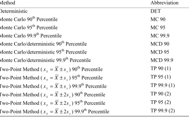
dose for carcinogens were estimated ...47 Table 9. Methods of risk estimation and their abbreviations. For each of the
probabilistic methods the 90th, 95th or 99.9th percentile value of the
Table 10. Intercept, slope and coefficient of determination (r2) for modified linear regression of intake doses by soil ingestion estimated by different methods, versus the standard deviation of the measured soil
concentration of non-carcinogens ...69 Table 11. Intercept, slope and coefficient of determination (r2) for modified
linear regression of intake doses by dermal absorption estimated by different methods, versus the standard deviation of the measured soil
concentration levels of non-carcinogens...69 Table 12. Intercept, slope and coefficient of determination (r2) for modified
linear regression of intake doses by inhalation estimated by different methods, versus the standard deviation of the modeled air concentration
of non-carcinogens...70 Table 13. Intercept, slope and coefficient of determination (r2) for modified
regression of intake doses by groundwater ingestion estimated by different methods, versus the standard deviation of the modeled
groundwater concentration of non-carcinogens...70 Table 14. Intercept, slope and coefficient of determination (r2) for modified
linear regression of intake doses by soil ingestion estimated by different methods, versus the standard deviation of the measured soil
Table 15. Intercept, slope and coefficient of determination (r2) for modified linear regression of intake doses by dermal absorption estimated by different methods, versus the standard deviation of the measured soil
concentration of carcinogens. ...73 Table 16. Intercept, slope and coefficient of determination (r2) for regression
of intake doses by groundwater ingestion estimated by different methods, versus the standard deviation of the modeled groundwater concentration
LIST OF FIGURES
Figure 1. Mean estimated intake dose for the soil ingestion exposure route for non-carcinogens. Method abbreviations are defined in Table 9. Values not annotated with the same letter are significantly different at p ≤ 0.05.
Bars represent the standard error ...53 Figure 2. Mean estimated intake dose for the dermal exposure route for
non-carcinogens. Method abbreviations are defined in Table 9. Values not annotated with the same letter are significantly different at p ≤ 0.05.
Bars represent the standard error ...55 Figure 3. Mean estimated intake dose for the inhaletion exposure route for
non-carcinogens. Method abbreviations are defined in Table 9. Values not annotated with the same letter are significantly different at p ≤ 0.05.
Bars represent the standard error ...56 Figure 4. Mean estimated intake dose for the groundwater ingestion exposure
route for non-carcinogens. Method abbreviations are defined in Table 9. Values not annotated with the same letter are significantly different at p ≤
0.05. Bars represent the standard error ...58 Figure 5. Mean estimated intake dose for the soil ingestion exposure route for
carcinogens. Method abbreviations are defined in Table 9. Values not annotated with the same letter are significantly different at p ≤ 0.05.
Figure 6. Mean estimated intake dose for the dermal exposure route
carcinogens. Method abbreviations are defined in Table 9. Values not annotated with the same letter are significantly different at p ≤ 0.05.
Bars represent the standard error ...63 Figure 7. Mean estimated intake doses for the groundwater ingestion exposure
route for carcinogens. Method abbreviations are defined in Table 9. Values not annotated with the same letter are significantly different at p ≤
CHAPTER 1
INTRODUCTION
The federal brownfields program was initiated in 1995 to stimulate redevelopment of the economic base of communities that have been negatively impacted by the loss of jobs and tax base that were previously associated with brownfields facilities (Davis and Margolis, 1997). Then Vice-President Al Gore emphasized this in June 1996 when he wrote in reference to brownfields (Davis and Margolis, 1997).
" . . . As we embark on this exciting new age, we cannot forget the many people and places left behind; people and places that want to join in the progress we are making. The estimated hundreds of thousands of abandoned and contaminated properties that are littered across our poorest communities – known as
'brownfields' – present a significant barrier to economic revitalization in our nation's cities. By encouraging the cleanup and redevelopment of these brownfields, the Clinton Administration is forging new ways to empower distressed communities and create jobs for their residents . . . "
Once brownfields have been redeveloped and placed back into the economy, localities can collect real-estate taxes and/or income taxes. The added revenues allow the communities to improve infrastructure, which provide new economic development opportunities thereby reversing the negative effects of urban decay. At the same time, brownfields redevelopment slows the development of virgin, undeveloped properties (greenfields), thus reducing the blight of urban sprawl.
The environmental contamination associated with a given brownfields facility creates a liability for potential redevelopers. This liability can eliminate the possibility of obtaining loans for the redevelopment of the facility. The financial risk of investing in brownfields is therefore a direct function of the potential for deleterious environmental effects posed by the contamination at the site to the surrounding community (Davis and
Margolis, 1997). This potential for harm is quantified by assessing the human health and environmental risk posed by the contamination at the site. Usually, as the health and environmental risks increase, the costs of removing these risks escalate and the likelihood of investment in these properties is decreased (Davis and Margolis, 1997).
The human health and environmental risks posed by contaminants at a
brownfields site are calculated using risk assessment algorithms that relate the level of contamination, toxicity, and exposure at the site (Davis and Margolis, 1997). The
primary objective of the risk assessment process is to determine whether current levels of contamination at the facility can result in unacceptable deleterious health effects and consequently require cleanup action or mitigation before redevelopment can proceed. Currently, the risk assessment process prescribed by the United States Environmental Protection Agency (USEPA) uses deterministic values for levels of contamination and exposure factors (i.e., intake rates, exposure time, exposure duration, body weight, etc.). These levels of contamination and exposure factors are then used to determine the
exposure level or intake dose. The intake dose is then combined with established toxicity values to determine the potential for future deleterious health effects (USEPA, 1989).
Variability and uncertainty are always associated with risk assessment since they are intrinsic to the contaminant levels, toxicity values, and the exposure factors used in the calculations. A quantitative assessment of the uncertainty and variability is an integral part of risk assessment (USEPA, 1989). In order to take into account such uncertainty and variability USEPA designed its deterministic risk assessment methodology to quantify the risk associated with the reasonable maximum exposure (RME). The RME is a conservative exposure level chosen within the 90th to 99.9th
percentile of the estimated range of possible exposures (USEPA, 1989). It has been suggested that the assumptions incorporated in the USEPA risk assessment process are too conservative and result in overestimating the RME and the estimated risk to the maximally exposed individual (Bogen, 1994). Additionally, combining several such upper-bound estimates in a multiplicative risk model would overestimate risk through the process termed as compounded conservatism (or “safety creep”). The outcome of the model would represent an upper bound that is greater than the input upper bounds (Bogen, 1994). Therefore, the risk assessment process may produce unreasonably high estimates of the risk posed by contaminants at the facility. If this occurs when assessing risk for brownfields, their redevelopment may be artificially stymied.
Recently introduced, probabilistic-based risk assessments are increasingly being used at Superfund sites to provide more complete estimates for the RME and its
associated risk. More complete estimates for the RME can lower remediation costs while still ensuring protection of human health and the environment (USEPA, 1999a). Unlike the deterministic approach to risk assessment that only provides an upper-bound estimate of risk, probabilistic-based risk assessments are feasible and cost-effective and can generate a more complete estimate of risk by better quantifying the degree of variability and uncertainty. However, Smith (1994) found that the deterministic approach and the probabilistic approach gave consistent risk estimates. Additionally, he found that the RME values for the deterministic approach were near the 95th percentile of the probabilistic estimates for the exposure routes he studied.
The probabilistic approach uses values of contaminant levels and exposure factors from probability distribution functions (pdfs) instead of the deterministic point estimates
in the traditional risk assessment approach. This method eliminates the problem of compounded conservatism associated with the deterministic method. The pdfs are generated using Monte Carlo simulations. Once the appropriate pdfs have been developed, values are selected at random from these distributions. These are then incorporated into the risk algorithms to calculate a single value of the environmental risk (Dakins et al., 1996). This process is then repeated thousands of times to develop a cumulative distribution of environmental risk. A value in the 90th to 99.9th percentile of this distribution is then used as the final risk value (USEPA, 1999a).
The Monte Carlo-based risk assessment method allows for sensitivity analysis to determine which parameters have the least impact on the risk outcome of a simulation. Pearson’s r or Spearman’s ρ can be used to test for sensitivity of the risk estimates to each parameter (Hamby, 1994; Palisade, 2000). The non-significant parameters can then be treated as deterministic variables thus reducing the number of distributions that must be developed and the number of Monte Carlo simulations that must be performed.
A less computationally tedious probabilistic method for estimating risk is
available but has never been applied in environmental risk assessment. This is the “two-point method” developed by Rosenblueth (1981), and Guymon et al. (1981). This method is based on estimates for the moments of a probability density distribution (Rosenblueth, 1975). The first two moments of the probability density distributions of the input random variables in the risk algorithms are used to estimate the mean and variance of the risk outcome. The two-point method requires less iterations than the Monte Carlo-based approach, thereby reducing the calculation-checking problem. It also reduces the problem of compounded conservatism. Use of Monte Carlo generated
distributions or the two-point method can provide better and more meaningful
quantification of the variability and uncertainty associated with the risk estimates than does the deterministic approach (USEPA, 1989).
The applicability and advantage of the probabilistic approach namely, the Monte Carlo-based and the two-point method, in quantifying variability and uncertainty in brownfields risk assessments need to be investigated. Since brownfields sites generally have fewer contaminants at lower concentrations than Superfund sites, there is the possibility that the Monte Carlo-based and the two-point method may not produce significantly different estimates for the reasonable maximum exposure compared to the deterministic method. However, if it can be shown that Monte Carlo-based and/or the two-point based risk assessments can better capture the uncertainty and variability inherent to the risk assessment process, the costs of remediation at brownfields sites can be reduced, and make brownfields redevelopment more attractive.
The primary objective of this study was to compare exposure and risk estimates obtained using the deterministic, Monte Carlo-based, and the two-point risk analysis method in relation to the variability and uncertainty in contaminant levels at selected brownfields facilities. Additionally, the sensitivity of the Monte Carlo risk estimates to the input parameters and their distributions were analyzed. Non-significant parameters identified by these analyses were treated as deterministic and used to develop and evaluate a hybrid Monte Carlo/deterministic method.
CHAPTER 2
LITERATURE REVIEW
2.1 Brownfields
The United States Environmental Protection Agency (USEPA, 1995) defines brownfields as: "abandoned, idled or underused industrial and commercial sites where expansion of redevelopment is complicated by real or perceived environmental
contamination that can add cost, time, or uncertainty to a redevelopment project." Davis and Margolis (1997) categorized brownfields as:
1) Sites that, despite needed remediation, remain economically viable, due to sufficient market demand.
2) Sites that have some development potential, provided financial assistance or other incentives are available.
3) Sites that have extremely limited market potential even after remediation. 4) Currently operating sites that are in danger of becoming brownfields because
historical contamination will ultimately discourage new investment and lending. This classification system indicates that brownfields redevelopment is a voluntary market-driven process. Because there is substantial risk associated with investing in a brownfields site, redevelopment will only be undertaken when there is a potential for substantial return on the investment (Davis and Margolis, 1997). Therefore, only the first two categories of brownfields are economically viable. Viable brownfields are
considered as under-utilized properties with actual or perceived environmental liabilities that, due to their inherently positive market attributes, may be economically redeveloped into productive assets (Davis and Margolis, 1997). Therefore, until such time as the market causes them to have value greater than the redevelopment cost, many brownfields will remain non-viable (Davis and Margolis, 1997).
The United States Government General Accounting Office estimates that there are 130,000 to 450,000 potential brownfields in the United States (Davis and Margolis, 1997). The cost to investigate and remediate all of these brownfields may be as high as $650 billion (Davis and Margolis, 1997). Although this estimated cost is high, the loss of tax dollars and lost wages is also high. The United States Conference of Mayors
conservatively estimated that their annual loss of tax revenues for 33 cities due to brownfields sites totaled $121 million. Using more realistic estimates, the projected losses were closer to $386 million (Davis and Margolis, 1997).
The stigma associated with environmental contamination at industrial and commercial brownfields reduces their market value and likelihood for redevelopment. This perception indirectly reduces employment and the tax base of the community in which they are located. In this context, Davis and Margolis (1997) considers stigma to be a persistent prejudice that any environmental contamination makes a property flawed, blemished, discredited, or spoiled. This prejudice exists primarily because of the real possibility that a site is contaminated with a chemical or material that has the potential to negatively impact human health. The effects of this stigma on a community with
brownfields are: (a) reduced potential for redevelopment because of fear of liability, resulting in loss of potential property-tax revenues, (b) unemployment due to reduced job base, (c) reduced need for public services and infrastructure, and (d) the disincentive for attracting new development (Davis and Margolis, 1997).
Available remediation standards can be used to determine when a brownfields site has been adequately remediated and thus remove the environmental stigma associated with the site (Davis and Margolis, 1997). Both remediation to background, or to
non-detectable levels of contamination, are often protective of human health and the environment; however, this approach often removes more contamination than is necessary resulting in increased remediation costs and decreased likelihood of redevelopment (Davis and Margolis, 1997).
To address the brownfields issues, the United States Environmental Protection Agency (USEPA) issued its "Brownfields Action Agenda" in January 1995. The action agenda was composed of four parts. First, the USEPA would put in place 50 pilot projects. Each project would receive $200,000 dollars over two years to help fund site evaluation and remediation (USEPA, 1995). Second, USEPA would clarify the liability and cleanup issues for prospective purchasers, lenders, and property owners. Included in this phase was the archiving of 24,000 sites that were slated for no further action from the CERCLIS database, (CERCLIS is the Comprehensive Environmental Response,
Compensation, and Liability Information System) which is the repository for information on hazardous waste sites, site inspections, preliminary assessments, and remediated hazardous waste (USEPA, 1995). Additionally, the USEPA would issue guidance that required the consideration of future land use when selecting remediation technologies at sites on the National Priorities List. Third, the action agenda would encourage public participation and community involvement. Fourth, the USEPA would establish an environmental education program to develop an environmentally conscious workforce (USEPA, 1995). Since the release of the “Brownfields Action Agenda” in 1995 all of the milestones have been accomplished including clarification of liability and cleanup issues, partnerships and outreach, job training, and brownfields pilots (USEPA, 2000a).
Five communities in Virginia received pilot project funds to aid in redevelopment of brownfields. These were Petersburg, Newport News, Shenandoah, Cape Charles, and Richmond. Petersburg and Newport News planned to use the funds to redevelop
depressed industrial areas in the inner city to spur economic development (USEPA, 2000b; USEPA, 1999b). Shenandoah planned to use the funds to redevelop a former iron furnace into recreational center and historical park (USEPA, 1998). Cape Charles used the funds to help redevelop a 25-acre town dump and surrounding lands into a
Sustainable Technology Industrial Park, a coastal dune preserve, and other natural areas. The project helped create 82 new jobs in a community where 27 percent of the 13,000 residents live below the poverty level (USEPA, 1999c). Richmond used the funds to assess and provide plans for the remediation of a 4.5-acre parcel of land. Whithall-Robins, a pharmaceutical company, subsequently spent nearly $2 million dollars to redevelop the land and was then given the site. The remediation allowed further development of the land that resulted in the creation of 250 new jobs and allowed 100 positions to remain in the Richmond area. The new facility generates an average of $100,000 per year in tax revenues (USEPA, 1999d).
2.2 Risk Assessment Methodology
2.2.1 Basic Concepts
The Comprehensive Environmental Response, Compensation, and Liability Act (CERCLA) of 1980 established the federal program that guides response to uncontrolled releases of hazardous substances into the environment. As authorized by CERCLA, the USEPA established protocols for assessing and remediating sites contaminated with
hazardous substances (USEPA, 1989). An essential part of this protocol was risk assessment. Risk assessment can be used to set remediation limits, lower remediation costs, lessen the stigma, and increase chances for redevelopment of a contaminated facility. Risk assessment is intended to be a process of gathering, organizing, and analyzing data to establish the probability of adverse health impacts from hazardous site conditions (Williams et al., 2000). The USEPA based its guidance for risk assessment on the National Research Council’s Risk Assessment in the Federal Government: Managing the Process (USEPA, 1989),already established guidance from other federal agencies
such as OSHA (Occupational Safety and Health Administration), FDA (Food and Drug Administration), and CPSC (Consumer Product Safety Commission), and its own accumulated experience conducting risk assessments at hazardous waste sites. The final guidance issued by USEPA was designed to (a) provide an estimate of risk and determine whether further action was warranted, (b) provide estimates of the highest level of a contaminant at a site that is not harmful to human health and the environment, (c) provide a means for comparing different possible remedial options, and (d) provide consistency in the methodology for determining human health risk from environmental contaminants (USEPA, 1989).
The National Research Council’s publication entitled Risk Assessment in the Federal Government: Managing the Process (NRC, 1983) established the process
currently used for conducting risk assessments and defined many of the operational terms. This document, sometimes referred to as the “Red Book”, also established the
basic risk assessment paradigm (NRC, 1994). This paradigm comprises a four-step process, namely, hazard identification, dose-response assessment, exposure assessment,
and risk characterization (Williams et al., 2000). The first two are sometimes grouped as toxicity assessment.
Hazard identification involves the determination of the potential impacts that exposure to a contaminant may have on the health of the exposed individual. These health impacts may be, but are not limited to, carcinogenesis, mutagenesis, neurotoxicity, hematotoxicity, nephrotoxicity, dermal and ocular toxicity, pulmonotoxicity,
immunotoxicity or hepatotoxicity (Williams et al., 2000). Although it is known that exposure to contaminants under some conditions can be toxic to humans, there is little direct evidence of causal relationships between exposure and toxicity for most chemicals. The most accurate method of determining toxicity would be to test the effects of exposure to contaminants directly on human subjects, which is not possible for obvious reasons. Therefore most assessments of health hazards are performed indirectly using
epidemiological studies, studies of accidental exposures, studies on laboratory animals, and comparison with pharmacokinetics of similar chemicals with known hazards (Williams et al., 2000).
The next step in the risk assessment paradigm is the dose-response assessment or the relationship between exposure level and the incidence and severity of deleterious health effects. Dose-response assessment not only takes into account the relationship of exposure to toxicity, but also the effects of exposure patterns, age, sex, and lifestyle factors (NRC, 1994). The dose-response relationship is often arrived at by extrapolation from high to low doses and from test animals to humans subjects (Williams et al., 2000).
Exposure assessment is the third step of the risk assessment paradigm and quantifies the intensity, frequency, and duration of human exposure to environmental
contaminants. Quantifying exposure can be simple or extremely complex. The concentration of a contaminant, to which an individual is exposed, can be directly
measured by collecting field samples and determining the concentration in the samples in an analytical laboratory. Exposure concentrations can also be modeled indirectly using the known physiocochemical relationships that control the movement of contaminants from source to receptor (USEPA, 1989).
The exposure concentration is dependent on the exposure pathway or any combination of potential exposure pathways (NRC, 1994). An exposure pathway describes how a given contaminant reaches and enters the human body. The exposure pathway therefore links the source and the type of contamination to the potentially exposed individual or population. For an exposure pathway to be complete there must be a source of contamination, a means of transport to the receptor, an exposure route into the receptor, and a potential for exposure by the given route (USEPA, 1989). Exposure pathways can be defined for contaminant movement through any combination of the air, water, and soil. Principal human exposure routes are ingestion, absorption and
inhalation.
The exposure frequency and duration, which depends on the exposure scenario, complicates the exposure assessment. Whether the exposed individual resides, works, or performs any other activity at the exposure point, dictates the estimated exposure
frequency and duration (USEPA, 1989). Generally, the residential scenario is associated with the greatest exposure and is therefore considered the most conservative exposure scenario. The residential exposure is therefore often considered for CERCLA sites.
However, in situations where the possibilities of future residential activities at a site are exceedingly small, the residential scenario will overestimate potential exposure or risk.
The final step of the risk assessment paradigm is risk characterization. In this step, the information from the first three steps is brought together to quantify the probability for deleterious health effects. Included in this step is the communication of the potential risk. This communication should include quantitative statements of all the variability and uncertainty that are associated with each of the three preceding steps and the final risk estimate (USEPA, 1989).
The methodologies for conducting risk assessments are described in the
operations manual entitled “Risk Assessment Guidance for Superfund Volume I: Human Health Evaluation Manual Part A” (USEPA, 1989). After appropriate data collection, the risk is calculated for each individual contaminant. The risk for both carcinogenic effects and noncarcinogenic effects of a contaminant can be calculated. The equation for
calculating carcinogenic risk is the product of the carcinogenic slope factor for the contaminant and its chronic daily intake dose expressed as the mass of a contaminant averaged over 70 years per unit body weight of the receptor. The slope factor converts the chronic daily intake value directly into the increase in the individual risk of
developing cancer (USEPA, 1989). The non-carcinogenic risk equation is the quotient of the intake of a contaminant of concern averaged over a specified period (also termed as the intake dose and expressed as mass per unit body weight per day) to its toxicity threshold value termed as the reference dose (RfD). The RfD is the intake of a contaminant below which there is not a substantial likelihood of toxicological effects
(USEPA, 1989). The ratio is called the hazard quotient or hazard index. Risk or hazard is therefore determined by the following equations (USEPA, 1989):
Carcinogen: Individual Lifetime ExcessCancer Risk=Intake×Slope Factor Non-carcinogen:
Dose
Reference
Intake
Hazard
=
In assessing risk for multiple contaminants the risk value is taken as the sum of the individual risk values (USEPA, 1989).
For carcinogens, the slope factor represents an upper bound estimate of the probability of a carcinogenic response per unit intake dose of a contaminant over an average lifetime of 70 years. The slope factor multiplied by the chronic daily intake value gives a maximum probability that an exposed individual will develop cancer from exposure to a contaminant over his or her lifetime (USEPA, 1989). Slope factor values are established by the Carcinogen Risk Assessment Verification Endeavor (CRAVE) workgroup, which was established to resolve the conflicting values that were being used by different program groups within USEPA (USEPA, 1989). These values are archived in USEPA’s Integrated Risk Information System (IRIS) database.
For non-carcinogens the RfD is determined using the No Observed Adverse Effect Level (NOAEL) or Lowest Observed Adverse Effect Lever (LOAEL) threshold values taken from toxicological studies of dose-response in test animals. The NOAEL is the highest level of intake by a given route that, statistically, has no adverse health impact on the treated population in relation to a control population in the study. The LOAEL is the lowest level of exposure that, statistically, has an adverse health impact on the subject population in relation to a control population (Williams et al., 2000). The NOAEL is then
magnitude. These uncertainty factors account for differences within the exposed population, differences between test animals and the exposed human population, values that were derived from subchronic studies versus chronic studies, and NOAEL values that were determined by extrapolation from the LOAEL values. An additional factor of 10 may be applied based on professional judgement to account for unspecified
uncertainties (USEPA, 1989).
Both carcinogenic slope factors and non-carcinogenic RfD’s are available in the IRIS database that is accessible on the USEPA Internet site http://www.epa.gov/iris/. Such values are also published in the Health Effects Assessment Summary Tables (HEAST) and the Agency for Toxic Substances and Disease Registry (ATSDR) toxicological profiles. Values from the IRIS database are preferred as they have undergone greater scrutiny than the other values (USEPA, 1989).
Both carcinogenic and non-carcinogenic risk calculations incorporate a value for intake, also termed as the administered dose or intake dose of the chemical. The generic equation for calculating the chemical intake dose by a given route is (USEPA, 1989):
AT 1 BW EFD CR C I= × × ×
Where: I = intake dose (mg kg-1 day-1); C = concentration in the medium of interest (mg liter-1, mg kg-1, mg m-3) ; CR= contact rate (liter day-1, kg day-1, m3 day-1); EFD = exposure frequency and duration and comprises two terms: exposure frequency (day year-1) and exposure duration (years); BW = body weight (kg); and AT = averaging time (day) (USEPA, 1989). The AT may be the same as the exposure duration or taken as some average lifetime. Because of the high uncertainty associated with the
the estimated range of the mean values for the chemical concentration in the generic equation (USEPA, 1989). Contact rate is an estimate of the amount of contaminated medium contacted per unit time. Exposure frequency and duration are combined to determine the total time of exposure. The USEPA suggests that these values be
determined from site specific information. However, default assumptions that are based on the exposure scenario (residential or industrial) are often used to specify these values. Body weight is estimated using the average body weight of the exposed population (USEPA, 1989). The averaging time for non-carcinogens is the same as the product of exposure frequency and duration in days. For carcinogens it is taken as an average lifetime of 70 years expressed in days.
For each exposure route there is a unique version of the generic equation that relates the amount of contamination in the media of concern to the intake dose expressed as mass of chemical per unit body weight per day. Four common intake dose models for residential exposure are listed below (USEPA, 1989):
(1) Residential Exposure: Ingestion of Chemicals in Soils
AT BW ED EF FI CF IR CS ) day kg Intake(mg -1 -1 × × × × × × = CS = Concentration in soil (mg kg-1) IR = Ingestion rate (mg soil day-1) CF = Conversion factor (10-6 kg mg-1)
FI = Fraction of IR attributable to contaminated soil (unitless) EF = Exposure frequency (days year-1)
ED = Exposure duration (years) BW = Body weight (kg)
AT = Averaging time (ED×365day year-1for non-carcinogens
(2) Residential Exposure: Dermal Contact with Chemicals in Soil AT BW ED EF ABS AF SA CF CS ) day kg Intake(mg -1 -1 × × × × × × × = CS = Concentration in soil (mg kg-1) CF = Conversion factor (10-6 kg mg-1)
SA = Skin Surface area available for contact (cm2) AF = Soil to skin adherence factor (mg soil cm-2) ABS = Absorption factor (unitless)
EF = Exposure frequency (days year-1) ED = Exposure duration (years)
BW = Body weight (kg)
AT = Averaging time (ED×365day year-1for non-carcinogens
and 70 years×365days year-1 for carcinogens)
(3) Residential Exposure: Inhalation of Airborne Chemicals
AT BW ED EF ET IR CA ) day kg Intake(mg -1 -1 × × × × × = CA = Concentration in air (mg m-3) IR = Inhalation rate (m3 hour-1) ET = Exposure time (hours day-1) EF = Exposure frequency (days year-1) ED = Exposure duration (years)
BW = Body weight (kg)
AT = Averaging time (ED×365day year-1for non-carcinogens
and70 years×365days year-1 for carcinogens)
(4) Residential Exposure: Ingestion of Chemicals in Drinking Water
AT BW ED EF IR CW ) day kg Intake(mg -1 -1 × × × × =
CW = Concentration in water (mg liter-1) IR = Ingestion rate (liter day-1)
EF = Exposure frequency (days year-1) ED = Exposure duration (years)
BW = Body weight (kg)
AT = Averaging time (ED×365day year-1for non-carcinogens
2.2.2 Variability and Uncertainty in Risk Estimation
Variability and uncertainty are intrinsic to each input parameter of the intake dose algorithms. The USEPA has provided definitions for variability and uncertainty as they apply to risk assessment. These definitions have been adopted by most of the risk
assessment community. They are (Finley and Paustenbach, 1994; NRC, 1994; Dakins et al., 1996; USEPA, 1999):
Variability: the true heterogeneity or diversity in a population. Uncertainty: a lack of knowledge regarding a population.
Uncertainty leads to inaccurate or biased estimates whereas variability leads to imprecise estimates. Uncertainty can be reduced with additional data. However, variability can only be better understood by the collection of additional data (Byrd and Cothern, 2000).
Sources of variability can be classified into three categories: spatial variability, temporal variability and inter-individual variability. The National Research Council (NRC, 1994) lists four ways to deal with these types of variability in risk estimation: (1) ignore the variability, (2) disaggregate the variability, (3) use the average, and (4) use maximum or minimum values. The first method is used when the variability is relatively low. The use of mathematical models or separating data into subpopulations are
appropriate ways to disaggregate the variability in order to better understand or reduce it. Using the sample average value is similar to ignoring variability except when the sample average value is a good estimator of the true population mean. The fourth approach is the most common method of dealing with variability in risk assessment (NRC, 1994).
However, the USEPA (1992a) cautions that the use of many extreme values could result in an inflated risk estimate.
Uncertainty is divided into three categories by the USEPA(1992a): (1) uncertainty regarding missing or incomplete information needed to fully define the exposure level and dose, (2) uncertainty regarding some input parameter, and (3) uncertainty regarding gaps in scientific theory required to make predictions on the basis of causal inferences. In the context of this study, uncertainty refers primarily to
parameter uncertainty. It is assumed that the exposure route is complete and known and that the exposure model is correct as defined by USEPA. Parameter uncertainty can be further categorized into random errors, systematic errors, and use of generic or surrogate data (Morgan and Henrion, 1990).
All estimates of parameter values contain both variability and uncertainty that confound one another (USEPA, 1997). If a quantity having high variability is assumed to be invariant, then even the most exact measurement scheme will appear to generate very uncertain results. In this case, the faulty measurement is ascribed to uncertainty when in fact it is due to variability (USEPA, 1997). For example, in estimating the average daily dose from ingestion of contaminated drinking water, it is possible to measure an
individual’s daily water consumption exactly, thereby eliminating uncertainty in the measured daily dose. The daily dose still has inherent day-to-day variability, due to changes in the individual’s daily water intake or the contaminant concentration in water. However, it is impractical to measure the individual’s dose every day. It has to be estimated based on sample measurements. Because the individual’s true average is unknown, it is uncertain how close the estimate is to the true value. Thus, the variability across daily doses has been translated into uncertainty (USEPA, 1997).
Taking conservative point estimates of the parameters and variables associated with exposure and toxicity provides a consistent, straightforward, and practical approach to dealing with variability and uncertainty in risk estimation. However, the USEPA mandate to be protective of human health and the environment, including sensitive sub-populations, contribute to a high degree of caution and conservatism in the estimation of risk. This approach has been termed the “better safe than sorry” response to variability and uncertainty (Byrd and Cothern, 2000). To be protective of a large portion of the population, USEPA chooses to bias on the side of safety.
2.2.3 Deterministic Risk Assessment
In general, deterministic models of physical processes consist of a function or a set of functions of one or more variables. In the deterministic approach to risk
assessment the function variables are taken as the mean, or some upper bound of a population distribution, or the distribution of sample means. The deterministic approach therefore ignores the actual variability and uncertainty that are associated with the individual input variables (Guymon and Yen, 1990). Variability and uncertainty are lumped by using conservatively chosen values for the density distribution of the input variables such that the estimated risk represents some upper bound value. However the range of possible risk values cannot be specified and therefore, no percentile ranking can be assigned to this upper bound value (USEPA, 1999).
The most important step in the deterministic risk assessment is estimation of the intake dose or reasonable maximum exposure (RME). USEPA defines the RME as the highest exposure that is reasonably expected to occur for current and future use at a site
(USEPA, 1989). The RME is generally estimated for each exposure route. However, multiple exposure routes can be combined in calculating the RME (USEPA, 1989).
Values for the inputs needed to estimate the RME and the final risk value by the deterministic method can be found in the “Exposure Factors Handbook” (USEPA, 1997) or in other guidance documents that have been released by the USEPA or State
Environmental Agencies. The concentration term is determined from site specific sampling data. The mean and standard deviation of these data are used to determine an upper (usually the 95th percentile) fiducial (confidence) limit for the sample mean. This practice is intended to ensure that the RME is not underestimated (USEPA, 1989).
The process to determine this upper fiducial limit for the mean has been laid out in Supplemental Guidance to RAGS: Calculating the Concentration Term released by
USEPA in May 1992 (USEPA, 1992b). This document outlines the method to estimate an upper bound of log transformed data. The method provided is taken from Land (1971) who derived the uniformly most accurate unbiased confidence interval procedure.
To determine the 95th percentile fiducial limit for the mean USEPA suggests that the contaminant concentration data should be tested to determine whether the data are normally or log-normally distributed. In lieu of determining the nature of the
distribution, USEPA suggests assuming that the data are log-normally distributed and use Land’s formula to calculate an upper confidence limit for the mean (USEPA, 1992b). Land’s formula uses the log-transformed data to calculate the mean and standard deviation of n sample data points and then calculates the upper confidence level of the
sample data using the following equation (USEPA, 1992b): − + + = − − 1 5 . 0 exp UCL 2 1 α 1 n H s s x x x α
Where xand sx are the mean and standard deviation of the log-transformed data and
α − 1
H is the H-statistic for confidence level 1−α. USEPA recommends a minimum of
four samples for estimating xand sx however, tables for the H-statistic present values
for sample sets with three samples (USEPA, 1992b).
The deterministic method has received much criticism for potentially over estimating the human health risk posed by a contaminated facility because of the use of overly conservative point estimates of risk model parameters. In addition, this method can result in “compounded conservatism”. Bogen (1994) stated: “ . . . Compounded conservatism (or “creeping safety”) describes the impact of using conservative upper-bound estimates of the values of multiple input variates to obtain a conservative estimate of risk modeled in an increasing function of those variates. In a simple multiplicative model of risk for example, if upper p-fractile (100pth percentile) values are used for each of several statistically independent input variates, the resulting risk estimate will be the upper p'-fractile of risk predicted according to that multiplicative model, where p' > p.”
Finley and Paustenbach, (1994a) stated that: “A major shortcoming [of the deterministic approach] lies in the fact that repeated use of upper-bounded point
estimates, as is recommended by the USEPA to calculate a reasonable maximal exposure (RME), typically leads to unrealistic estimates of health risk and unreasonable clean-up goals.” The issue of using overly conservative point estimates was addressed in two
appendices to “Science and Judgment in Risk Assessment” (NRC, 1994). Appendix N-1 written by Adam M. Finkel and entitled “The Case for ‘Plausible Conservatism’ in Choosing and Altering Defaults” defended the USEPA approach to determining default
two criteria, scientific plausibility and whether it is conservative and protective of human health (NRC, 1994). Appendix N-2 written by Roger O. McClellan and D. Warner North and entitled “Making Full Use of Scientific Information in Risk Assessment,” advocates the use of “Plausible Conservatism” for choosing and altering default assumptions. Appendix N-2 suggests that more site-specific information should be incorporated into risk assessments to reduce possible default parameter conservatism (NRC, 1994).
There are several benefits of using point estimates of input variables for risk assessment. The procedure of risk assessment using point estimates is simple and
accessible. Once contamination data have been collected applying the model of exposure assessment is very straightforward. Most inputs to the model can be found on the
USEPA web site (http://www.epa.gov). In addition, regulators readily accept the risk assessment based on point estimates. This method has been used for more than 15 years, and there is a wealth of guidance for both conducting and reviewing deterministic risk assessments (USEPA, 1999a). Running the risk assessments in reverse can provide site concentration levels for a specified risk value. These levels can then be used to screen which site contaminants should be considered for further investigation (Finley and Paustenbach, 1994).
2.2.4 Probabilistic Risk Assessment
Probabilistic risk assessment is a generic term for risk assessments that use probability models for the input variables instead of point values. This approach makes possible quantitative analysis of variability and uncertainty associated with the input variables (USEPA, 1999a). The ability to quantitatively analyze variability and
uncertainty allows the risk manager to chose a regulatory level of concern that will be exceeded with some known probability in comparison with deterministic methods that provide an estimate of risk that represents a high end value with unknown probability (USEPA, 1999a).
Probabilistic risk assessment makes use of the same basic algorithms that were already described and used for deterministic risk assessment. However, the probability distribution of possible intake doses is determined before multiplying by the toxicity value. This results in a density distribution of risk values unlike the deterministic
approach, which yields a single estimate that represents the risk associated with the RME (USEPA, 1999a). The USEPA does not recommend the use of probability distributions for the toxicity variable, because the data are not sufficient to generate distributions that represent its variability and uncertainty (USEPA, 1999a).
For the purposes of risk management decisions, the USEPA suggests using values that fall between the 90th and 99.9th percentile of the risk output distribution, termed as the RME range (USEPA, 1999a). The value that is chosen from this range should reflect the confidence in the input parameters to the probabilistic model, and the end use of the site being investigated, to ensure it is protective of human health and the environment (USEPA, 1999a).
The probabilistic approach to calculating risk has been thoroughly critiqued. Some of the disadvantages have been outlined by the USEPA (1999a). There may not be sufficient information about the variability and uncertainty to specify the appropriate distribution of the exposure variables. Using probabilistic methods require significantly more resources to perform the risk assessment, interpret the results, and present the final
report. USEPA also cautions against a false sense of accuracy in the risk estimates, since probabilistic methods only quantify variability and uncertainty, they are not reduced or eliminated.
Monte Carlo techniques are most frequently used to develop the input probability distributions needed for risk estimation. Burmaster and Anderson (1994) provide 14 principles of good practice for using Monte Carlo techniques in risk assessment. They reiterate USEPA’s caution about use of inadequate data or inappropriate distributions for the input variables. Additionally, it is recommended that the input distributions be shown both numerically and graphically to convey the full sense of the distribution properties. Finally, they caution that enough iterations should be run to demonstrate that the tails of the simulated distribution stabilize.
Finley and Paustenbach (1994a) discussed the benefits of Monte Carlo-based probabilistic exposure assessment. They state that the deterministic method often predicts risks that are representative of the 99.9th percentile for the range of values rather than the intended 50th or 95th percentiles. The USEPA points out that probabilistic methods can provide more insight into the characteristics of the entire risk distribution. Also, probabilistic methods allow for value-of-information analysis and sensitivity analysis for identifying the input variables that strongly influence the outcome of the probabilistic risk assessment (USEPA, 1999a).
The methods for conducting Monte Carlo-based risk assessments are outlined in “Risk Assessment Guidance for Superfund Volume III: Process of Conducting
Probabilistic Risk Assessment (Part A)” (USEPA, 1999a). In Monte Carlo-based risk analysis, the upper-bound estimates of the variables used in the deterministic intake
model are replaced with probability distribution functions (pdfs) that describe the entire population of the particular variable (Dakins et al., 1996). A set of numbers for input to the intake model is obtained by randomly selecting a value from the pdf for each of the input variables. This set of values is then used to calculate one possible intake dose and an associated risk value. This process is iterated n times. The n possible values are
combined to create pdfs of the intake dose and predicted risk. From the intake dose distribution, risk managers can select the level of conservatism (usually between the upper 90th and 99.9th percentiles of the distribution) that is appropriate to specify the reasonable maximum exposure (Dakins et al., 1996).
Random selections of values from the pdf can be performed using one of three possible sampling techniques (McKay et al., 1979). The first is random sampling where values are drawn at random from each of the input distributions. This objective is accomplished by using computer algorithms to generate series of pseudo-random numbers. These series are usually sufficiently long so that, for the purposes of risk assessment, they can be considered infinitely long (Press, 1986). The second method for selecting values from the input pdf is stratified sampling where the pdf is divided into N sections and a random sample is drawn from the Nth division of each pdf (McKay et al., 1979). The third method is Latin Hypercube Sampling, which is a subset of stratified sampling where each of the N sections of the pdf have the same marginal probability distribution (McKay et al., 1979). The latter two methods allow for faster convergence in the tails of the output distribution for the intake dose and risk (Burmaster and Anderson, 1994).
Monte Carlo-based risk assessment has been criticized because it is computationally more complicated and, therefore, more time consuming than
deterministic risk assessment. Thousands of iterations are required so that the tails of the output pdf will stabilize, thus making quality control and calculation checking difficult. Even with this difficulty, USEPA has stated that “Monte Carlo simulation is clearly superior to the qualitative procedures currently used to analyze uncertainty and variability” (USEPA, 1997b) and has recently published guidance for conducting
probabilistic risk assessments (USEPA, 1999a). The Virginia Department of Environment Quality has provided some guidance for performing probabilistic risk assessment in its Risk Exposure Analysis Management System (REAMS) guidance document (VADEQ, 1994).
Monte Carlo-based risk analysis may provide a more comprehensive estimation of environmental risk. By using the distribution rather than deterministic estimates of an input variable or parameter, variability and uncertainty can be accounted for
quantitatively. By performing Monte Carlo-based risk analysis, risk managers can examine the full distribution of risk, and select a better reasonable maximum exposure value (USEPA, 1999a). Monte Carlo-based risk assessment obviates the arguments in the deterministic approach concerning the choice of a point estimate. It also eliminates the problem of compounded conservatism that arises from the multiplying several upper bound estimates or fiducial limits. Sensitivity analysis is more meaningful in conjunction with Monte Carlo-based analysis than with deterministic risk assessments (Finley and Paustenbach, 1994a).
Some of the drawbacks of the Monte Carlo-based approach can be overcome by using a combination of the probabilistic and deterministic methodology. In this
approach, sensitivity analysis is first used to determine which input distributions can be treated as deterministic, based on their impact on the outcome of the model. Sensitivity analysis measures the relative impact that a variable has on the outcome of a model (Hamby, 1994), and can be used to determine which input variable distribution has the greatest impact on the calculated risk. Because inputs with greater variability and/or uncertainty have a greater impact on model outcomes in Monte Carlo assessments, sensitivity analysis can indicate which variables or parameters need further investigation and refinement. If an input parameter distribution has a relatively large impact on the model outcome, this indicates that its variability and/or uncertainty may be large. If the uncertainty is large, additional information may reduce this uncertainty and increase the accuracy of the risk estimate (Finley and Paustenbach, 1994a).
Generally, sensitivity analysis is performed by relating the change in a parameter to the corresponding change in the outcome of the model. Several measures of this relationship have been used in risk assessment. These are the Sensitivity Ratio, Pearson Correlation Coefficient, and Spearman Rank Order Correlation Coefficient (Palisade, 2000). The Sensitivity Ratio is the change in the output of a model divided by change in an input variable. Pearson Correlation Coefficient measures the strength and direction of the linear association between the values. Spearman Rank Order Correlation Coefficient is a nonparametric measure of the strength and direction of association of the ranks of two quantitative variables (USEPA, 1999a).
Once it has been determined which input distributions have negligible impact on the output distribution, these parameters can be treated as deterministic values (USEPA, 1999a). By treating these inputs as deterministic values, the number of pdfs is reduced. Thus the calculation checking problems and quality control problems are reduced, while the majority of the information concerning variability and uncertainty is retained in this combined probabilistic/deterministic approach.
Another approach that can make the probabilistic risk assessment methodology less computationally tedious is the “two-point” method (Guymon et al., 1981). However, it has never been used in environmental risk assessment. The two-point method is so named because it uses the first two moments of the random variables (X1, X2, . . .Xm) of a
well-behaved multivariate distribution function Y = f(X1,X2, . . . Xm) to approximate the
moments of Y (Rosenblueth, 1975). Only the mean and the standard deviation of each variable are needed instead of the entire probability density function. This reduces the required knowledge about the independent variables. Additionally, the two-point method reduces the number of iterations required to estimate an upper bound of the risk
distribution. The two-point method has been applied to frost heave models (Guymon et al., 1981) and groundwater flow models (Guymon and Yen, 1990; Yen and Guymon, 1990)
Rosenblueth (1975) developed the two-point method. ConsiderX and Y are real
random variables and Y is a well-behaved function of X , with X the expectation, σx the standard deviation, and νxthe skewness coefficient of X . Rosenblueth (1975) defines the impulse probability density functions f+(X)=P+δ
(
X + x+)
,(
−)
−
− X =P X −x
Dirac delta function and x+and x−are arbitrary values of X greater than and less than X respectively. This implies that the nth moment E(Yn) of Y = f+(X)+ f−(X) is given by (Rosenblueth, 1975): n n n y P y P Y E( )= + + + − −
where )y+ =δ(X +x+ , )y− =δ(X −x− . This also implies P+, P−, x+, x− must satisfy
the following simultaneous equations (Rosenblueth, 1975): 1 = + − + P P X x P x P+ ++ − − =
(
)
2 2 2 ) (x X x P X x P+ + − + − −− =σ(
)
3 ( )3 3 3 x x X x P X x P+ + − + − −− =ν σwhose solution is (Rosenblueth, 1975)
− − = + 2 ) 2 ( 1 1 1 1 2 1 x v P m + − = −P P 1 − + + = X + P P x σx / + − − = X − P P x σx /
Here νxis unknown and is assumed to be zero (Rosenblueth, 1975). This implies 2
1 = = −
+ P
symmetric, even function ofX . The mean, standard deviation, and coefficient of
variation for Y = f+(X)+ f−(X) is then given by (Rosenblueth, 1975):
2 − ++ =Y Y Y 2 − + − = Y Y Y σ − + − + + − = Y Y Y Y VY
where )Y+ =Y(x+ and )Y− =Y(x− and Vyis the coefficient of variation.
For more than one independent variables:. ) ( ),... ( ) ( ) ,... , (X1 X2 Xm f X1 f X2 f Xm f Y = = ⋅ ⋅
Assuming that none of these m variables are correlated, the nth moment of Y can be
calculated by:
[ ]
[
(
) (
) (
)
n]
m n m n m m n y y y Y E ' ... ' ... ' ... 2 1 − − + − + + + + = where[ ]
n YE is the nth moment of Y , m is the number of independent random variables,
and the notation y’++. . . m indicates all permutations of the set:
} ,... , { ' x1 s1 x2 s2 xm sm y = ± ± ±
where xiis the mean, and siis the standard deviation of the i
th independent random
variable (Guymon et al., 1981). From this relationship the mean of Y =E(Y) is calculated when n is one and the variance as VAR [(Y)] = E(Y2) - [E(Y)]2.
The two-point method requires 2m iterations, which will be less than that required for the Monte Carlo-based simulation until the number of independent, random variables
exceeds 13. This method will also eliminate the problem of compound conservatism inherent in the deterministic method.
CHAPTER 3
MATERIALS AND METHODS
3.1 Brownfields Sites and Contaminant Data
In order to quantify the variability and uncertainty in risk estimates for individual contaminants using deterministic and probabilistic approaches a reliable set of
contaminant data on brownfields sites were required. Risk estimates for multiple contaminants were not addressed in this study. This data set was developed using the Pennsylvania Department of Environmental Protection (PADEP) Land Recycling
Program list of completed brownfields sites. This list is updated quarterly. The list at the end of the fall quarter of 2000 was used to develop the data set. The Fall 2000 list
consisted of 633 completed brownfields. These sites were sorted into four groups based on whether the site was closed to background, statewide generic standards, site-specific, or industrial standards. Only the sites that were closed to statewide health, site-specific, and industrial standards were used in this study. From this reduced list, 30 sites were selected at random. The RAND function in EXCEL® (Microsoft Co., Redmond, WA) was used to generate 30 pseudo-random numbers. These numbers were then matched to specific sites on the numerically ordered reduced list. A request was make to PADEP to gain access to the files on these 30 sites. Ten of these sites did not have sufficient data or the PADEP could not find the files. The sites that were included in the study are
presented in Table 1. One site, Exxon SGH Specialty Products, was listed as one facility but had two separate cleanup programs. Each of these was treated separately, giving a total of 21 brownfields sites used in this study.
The files on these 21 sites were archived in the specific PADEP Region listed in Table 1. This necessitated two separate trips to Pennsylvania to do the record reviews and collect data. Photocopies were made of all pertinent data in the files at the PADEP regional offices. The data were then manually transcribed into EXCEL® (Microsoft Co., Redmond, WA) spreadsheets. The data were carefully scrutinized for completeness and consistency. Since the PADEP has already approved these data for use in their risk assessments, and they had already been validated in accordance with USEPA guidelines as required under Pennsylvania’s Land Recycling Program, a complete data validation was not needed.
Table 1. Twenty-one sites taken from Pennsylvania's Land Recycling Program list of completed brownfields.
Region County Town Facility
Northeast Lackawanna Carbondale Carbondale Railyards
Northwest Lawrence New Castle Johnson Bronze
Northwest Erie Erie City Erie City Iron Works
Southcentral Blair Hollidaysburg GPU, Hollidaysburg Pole Yard Southcentral Cumberland LeMoyne Borough Conewago Contractors Inc. Southcentral Lebanon West Lebanon Aqua Chem Inc. Cleaver Brooks Southeast Bucks Upper Makefield Moyer Packing
Southeast Bucks Warrington Home Depot
Southeast Bucks New Britain Township Chalfont Plaza Assoc. LP Southeast Bucks Perkasie Borough LeNape MFG Co.
Southeast Chester Phoenixville Borough West Co.
Southeast Delaware Chester Peco Tighman St Gas PLT
Southeast Delaware Chester SMK Speedy Intl. Inc.
Southeast Delaware Springfield Township Sunoco 0004 8751 Southeast Delaware Upper Darby
Township
Bond Shipping Center Southeast Philadelphia Philadelphia Van Waters and Rogers Southeast Philadelphia Philadelphia Flying Carport Inc. Southeast Philadelphia Philadelphia American Cable Co.
Southwest Allegheny Pittsburgh Exxon SGH Specialty Products*
Southwest Beaver Freedom Ashland Chemical Co.
Measured contaminant levels in the soil at these sites were used to estimate exposure concentrations in the air and groundwater. The concentrations were calculated using the procedures provided in the “Soil Screening Guidance: Technical Background Document” (USEPA, 1996). These procedures use several conservative assumptions to provide conservative estimates of air and groundwater concentrations. Most
significantly, it is assumed that the soil is an unlimited source of the contaminant (USEPA, 1996). Also, the contaminant is assumed to be applied over a square area of half an acre that will provide conservative estimates for larger sites because of the unlimited source assumption. These assumptions simplify the underlying mass transfer models and reduce the need for large quantities of site-specific data that are often not available (USEPA, 1996).
The calculation of exposure concentrations for the inhalation route is divided into two possible mechanisms: inhalation of vapors for volatile contaminants and inhalation of contaminants adsorbed onto suspended soil particles for non-volatile contaminants. The concentration of contaminant in the air for volatile and non-volatile contaminants is calculated using the volatilization factor (VF) or the particulate emission factor (PEF), respectively. Both the VF and PEF are based on two models: one that estimates vapor or particulate emissions from the soil and one that estimates subsequent dispersion.
The emissions model for volatile contaminants is a simplification of the soil to atmosphere volatilization model developed by Jury et al. (1984) assuming that there is an unlimited source and no chemical and biological degradation. This model is based on transport theory outlined by Jury et al. (1983) and assumes 5 conditions. These are: (1) soil properties are constant with depth, (2) the contaminant partitioning on the soil
follows a linear, equilibrium adsorption isotherm, (3) partitioning of the contaminant between the soil solution and air follows Henry’s law, (4) uniform initial concentration of contaminant in the soil, and (5) volatilization occurs through a stagnant air layer above which the contaminant concentration is zero (Jury et al., 1983). Additionally, it is assumed that the volatilization has reached steady state (USEPA, 1996).
The emissions model of the PEF is taken from Cowherd et al. (1985) who based his equation on the PM10 emission factor proposed by Gillette (1981). Calculation
of the PEF requires that there is an unlimited reservoir of contaminated erodible particles. It is also assumed that the soils remain dry at all times, there is no variation in
meteorology between the source and receptor, that the meteorology at the site can be represented as average values for the surrounding region, there is no deposition or reaction at the ground surface, and that emissions are uniformly distributed over the site. Additionally the level of contamination in the suspended particulate matter is assumed to be the same as the bulk soil (USEPA, 1996).
USEPA Office of Air Quality Planning and Standards developed the dispersion model for estimating ambient air concentrations from low or ground level, non-buoyant sources of emissions. The Industrial Source Complex Model platform was used to determine generic dispersion values for different regional meteorological conditions (USEPA, 1996). This dispersion model is integrated with either the vapor or particulate emission models resulting in single equations for estimating the VF and PEF. The procedures for estimating air concentrations from soil concentration are as follows:
Contaminant concentration in the air (USEPA, 1996)
VF CS
CA= × 1 for volatile compounds
PEF CS
CA= × 1 for non-vola