by
http://ssrn.com/abstract=1654506
David Dillenberger and Kareen Rozen
“Disappointment Cycles”
PIER Working Paper 10-028
Penn Institute for Economic Research Department of Economics University of Pennsylvania 3718 Locust Walk Philadelphia, PA 19104-6297 [email protected] http://economics.sas.upenn.edu/pier
Disappointment Cycles
∗
David Dillenberger
†University of Pennsylvania
Kareen Rozen
‡Yale University
August 2010
AbstractWe propose a model of history dependent disappointment aversion (HDDA), allowing the attitude of a decision-maker (DM) towards disappointment at each stage of aT-stage lottery to evolve as a function of his history of disappointments and elations in prior stages. We establish an equivalence between the existence of an HDDA representation and two documented cogni-tive biases. First, the DM overreacts to news: after suffering a disappointment, the DM lowers his threshold for elation and becomes more risk averse; similarly, after an elating outcome, the DM raises his threshold for elation and becomes less risk averse. This makes disappointment more likely after elation and vice-versa, leading to statistically cycling risk attitudes. Second, the DM displays a primacy effect: early outcomes have the strongest effect on risk attitude. “Gray areas” in the elation-disappointment assignment are connected to optimism and pes-simism in determining endogenous reference points.
Keywords: history dependent disappointment aversion, disappointment cycles, overreaction
to news, primacy effect, endogenous reference dependence, optimism, pessimism
JEL Codes:D03, D81, D91
∗First version June 2010. We are grateful to Simone Cerreia-Vioglio for helpful conversations. We also benefitted
from comments and suggestions by Larry Samuelson.
†Department of Economics, 160 McNeil Building, 3718 Locust Walk, Philadelphia, Pennsylvania 19104-6297. E-mail: [email protected]
‡Department of Economics and the Cowles Foundation for Research in Economics, 30 Hillhouse Avenue, New Haven, Connecticut 06511. E-mail: [email protected]. I thank the NSF for generous financial support through grant SES-0919955, and the economics departments of Columbia and NYU for their hospitality.
Once bitten, twice shy. — Proverb
1. Introduction
Consider two people in a casino who have the same total wealth and the same utility for monetary prizes. One person has already won several games at the roulette wheel; the other person lost at those games. Will these individuals’ attitudes toward further risk be the same, or might they depend on whether they had previously won or lost? Consider now a third person who has just won $100 in a lottery between $100 and $x. Even though his winnings are $100 in both cases, could his attitude
to future risk depend on whether x, the alternate outcome, corresponded to winning or losing a
thousand dollars?
There is experimental evidence that the way in which risk unfolds over time affects risk atti-tudes (e.g., Thaler and Johnson (1990), Gneezy and Potters (1997), Bellemare, Krause, Kr¨oger, and Zhang (2005), and Post, van den Assem, Baltussen, and Thaler (2008)); and moreover, that
individ-uals are affected by unrealized outcomes, a phenomenon known as counterfactual thinking(e.g.,
Kahneman and Tversky (1982), Kahneman and Miller (1986), and Medvec, Madey and Gilovich (1995)). Thaler and Johnson (1990) suggest that individuals become more risk averse after negative experiences and less risk averse after positive ones. Post, van den Assem, Baltussen, and Thaler (2008) suggest that individuals are more willing to take risks after extreme realizations. The latter two studies consider settings of pure chance—suggesting that the effects therein are psychologi-cal in origin, and are not the result of learning about oneself or one’s environment. However, a psychological effect on risk attitude may potentially exist in more general contexts; for example, among NBA basketball players, Rao (2009) shows that “a majority of the players...significantly change their behavior in response to hit streaks by taking more difficult shots” but that “controlling for shot conditions, players show no evidence of ability changing as a function of past outcomes.” In this paper, we propose a model of history-dependent disappointment aversion (HDDA) over
T-stage lotteries that permits risk attitudes to be shaped by prior experiences. Our building block is
Gul (1991)’s model of disappointment aversion for one-stage lotteries, in which a decision maker (DM) categorizes monetary outcomes of a lottery as elating or disappointing, and calculates his “expected utility” of a lottery while uniformly overweighting the disappointing outcomes. A prize is elating (disappointing) if its utility is weakly larger than (strictly smaller than) the utility of the lottery as a whole. For a fixed utility over monetary prizes, the DM’s risk aversion is increasing
in his disappointment aversion coefficient (the additional weight he places on disappointing
disappointments and elations affect the evolution of risk attitude (by way of the disappointment aversion coefficient).
To ease exposition, we begin by describing our HDDA model in the simple setting of temporal lotteries, in which no intermediate choices may be taken while risk unfolds; later, the model is extended in a dynamically consistent manner to the setting of stochastic decision trees, with our results carrying over. In the HDDA model, the DM endogenously characterizes each realization of a temporal lottery (itself a sublottery) as elating or disappointing. At each stage, the DM’s history is the preceding sequence of elations and disappointments. Each possible history corresponds to a (potentially different) disappointment aversion coefficient. The HDDA model consists of a continuous and increasing utility function over monetary prizes, a set of potential disappointment aversion coefficients, and a history assignment mapping sublotteries to those coefficients. The value of a lottery is determined recursively using the model of disappointment aversion and the appropriate disappointment aversion coefficient for each history, with the requirement that the
history assignment for all sublotteries beinternally consistent. Internally consistency requires that
if a sublottery is considered elating (disappointing), then its value should indeed be weakly larger than (strictly smaller than) the value of the sublottery from which it emanates.
We do not place an explicit restriction on how histories map to disappointment aversion co-efficients (that is, how risk aversion should depend on the history). Nonetheless, we show that the HDDA model predicts two well-documented cognitive biases; and that these biases are suffi-cient conditions for an HDDA representation to exist. First, in accordance with the experimental
evidence cited above, the DM overreacts to news: he becomes less risk averse after positive
ex-periences and more risk averse after negative ones. Second, the DM displaysprimacy effects: his
risk attitudes are disproportionately affected by early realizations. Sequencing biases, especially the primacy effect, are robust and long-standing experimental phenomena (early literature includes Anderson (1965)). The primacy effect has implications for the optimal sequencing of information to manipulate behavior; for example, we study how a financial advisor trying to convince a DM to invest in a risky asset should deliver mixed news.
HDDA also has predictions for the DM’s endogenous reference levels. In particular, the model
predicts disappointment cycles. The DM increases the threshold for elation after positive
expe-riences and lowers it after negative expeexpe-riences. This makes disappointment more likely after elation, and vice-versa, leading to statistically cycling risk attitudes. The psychological literature, in particular Parducci (1995) and Smith, Diener, and Wedell (1989), provides support for the
pre-diction that elation thresholds increase (decrease) after positive (negative) experiences.1
For some lotteries, there may be more than one internally consistent assignment of histories. The DM’s history assignment is revealed by preferences. Because the DM’s choice of assignment
may affect his utility from a temporal lottery, we view anoptimistas a DM who always chooses the
“most favorable” interpretation (when more than one interpretation is possible) and apessimistas
a DM who always chooses the “least favorable” interpretation. This notion of optimism and pes-simism is distinct from previous notions which identify optimism and pespes-simism with the choice of (distorted) beliefs; for example, see B´enabou and Tirole (2002), Chateauneuf, Eichberger, and Grant (2007), or Epstein and Kopylov (2007).
Applied work suggests that changing risk aversion helps to understand several empirical phe-nomena. Barberis, Huang, and Santos (2001) allow risk aversion to depend on prior stock market gains and losses `a la the experimental evidence of Thaler and Johnson (1990), and show that their model is consistent with the well-documented equity premium and excess volatility puzzles. Rout-ledge and Zin (2010) address the same empirical phenomena, proposing a generalization of Gul’s model for one-stage lotteries that allows for a subset of lotteries to be valued under expected utility theory. Applying their model recursively (and without history dependence), they show that the preference parameters and transition probabilities between low and high states of the economy can be calibrated to generate effective risk aversion that is countercyclical.
In the HDDA model, risk attitudes are affected by “what might have been.” In many theories of choice over temporal lotteries, risk aversion could depend on the passage of time, wealth ef-fects or habit formation in consumption; see Kreps and Porteus (1978), Chew and Epstein (1989), Segal (1990), Dillenberger (2010), and Rozen (2010), among others. We study how risk attitudes are affected by the past, independently of such effects as above. Our type of history dependence is conceptually distinct from models where contemporaneous and future beliefs affect contempo-raneous utility (that is, dependence of utility on “what might be” in the future). This literature
includes Caplin and Leahy (2001), Epstein (2008), and K¨oszegi and Rabin (2009).2
The remainder of this paper is organized as follows. Section 2 formalizes the domain of tempo-ral lotteries. Section 3 provides a primer on the model of disappointment aversion of Gul (1991). Section 4 formalizes the HDDA model and contains our main results for temporal lotteries.
Im-(decreased) satisfaction with subsequent modest events....Thus, the occasional experience of extreme negative events facilitates the enjoyment of the modest events that make up the bulk of our lives, whereas the occasional experience of extreme positive events reduces this enjoyment.”
2In K¨oszegi and Rabin (2009), given any fixed current belief over consumption, utility is not affected by prior history (how that belief was formed). Their model, which presumes the DM is loss averse over changes in successive beliefs, could be generalized to include historical differences in beliefs, which would then affect utility values but not actual risk aversion due to their assumption of additive separability; we conjecture that one could relax additive separability to find choices of parameters and functional forms for their model that replicate the primacy effect and overreaction to news predicted by HDDA.
plications of HDDA are studied in Section 5. Section 6 extends our model and results to a setting where intermediate actions are possible. Axiomatic foundations for HDDA are provided in Section 7. Section 8 discusses directions for further research.
2. Framework:
T
-stage lotteries
We begin by studying the simple setting ofT-stage lotteries; in Section 6 we extend the setting to
stochastic decision trees.
LetX= [w,b]⊂Rbe a bounded interval of monetary prizes, wherewis the worst prize andbis
the best prize. The set of all simple lotteries (i.e., having a finite number of outcomes) overXis
de-notedL(X), or simplyL1. Elements of L1are one-stage lotteries. We reserve lowercase letters
for one-stage lotteries; typical elements ofL1are denoted p,q, orr. The probability of a monetary
outcomex under p is denoted p(x). A typical element p has the form hp(x1),x1;. . . ,p(xm),xmi.
The degenerate lotteryδx∈L1gives the prizexwith probability one.
Two-stage lotteries are simple lotteries over L1. The set of two-stage lotteries is denoted
L(L(X)), or simplyL2. A typical elementP∈L2has the form
P=hα1,p1;...;αm,pmi,
where for every j, pj∈L1, andαj∈[0,1], with∑mj=1αj=1.
ForT ≥3, the set ofT-stage lotteries,LT, is defined by the inductive relationLT =L LT−1.
A typical elementPT ofLT has the form
PT =α1,P1T−1;...;αm,PmT−1
,
where each PTj−1 ∈LT−1 is a (T −1)-stage lottery. If PT−1
j is the outcome of PT, then all
remaining uncertainty is resolved according toPTj −1. To simplify notation, we use the superscript
T only whenT ≥3. The degenerate lotteryδTx ∈LT gives the lotteryδTx−1with probability one
(i.e.,xis received with probability one afterT stages).
To avoid redundancy, our notation for anyt-stage lottery implicitly assumes that the elements
3. Disappointment aversion
The model of disappointment aversion proposed by Gul (1991) characterizes a DM’s preferences
over the set of one-stage lotteries,L1. For any lottery p∈L1, consider its certainty equivalent
CE(p). This is the monetary prize which the DM considers to be indifferent to pitself. The
lot-tery p may contain prizes in its support which are weakly preferred to p; receiving such a prize
is considered an elatingoutcome. The lottery pmay also contain prizes in its support which are
worse than p; receiving such a prize is adisappointingoutcome. Gul’s model of disappointment
aversion considers a DM who values lotteries by taking their “expected utility,” except that disap-pointing outcomes get a uniformly greater weight that depends on the value of a single parameter
β, thecoefficient of disappointment aversion. SinceCE(p)depends on all the prizes in the support
of p, the division into elating and disappointing outcomes (known as the elation-disappointment
decomposition), is determined endogenously, as seen in the utility representation below.
Formally, the disappointment aversion model consists of an increasing and continuous utility
function over prizes u:X →R and adisappointment aversion coefficient β ∈(−1,∞) such that
the value of a lottery p,V(p;u,β), uniquely solves
V(p;u,β) = ∑{x|u(x)≥V(p;u,β)}
p(x)u(x) + (1+β)∑{x|u(x)<V(p;u,β)}p(x)u(x) 1+β∑{x|u(x)<V(p;u,β)}p(x)
. (1)
The term in the denominator normalizes the weights on the prizes so that they sum to one. When
β >0, disappointing outcomes are overweighted and the DM is called disappointment averse.
When β <0, disappointing outcomes are underweighted and the DM is called elation seeking.
Whenβ =0, the model reduces to the model of expected utility.
In Gul’s model, risk aversion is captured by both the concavity of u (as in expected utility)
and the value ofβ. In particular, Gul (1991, Proposition 3) shows that the DM is risk averse if
and only ifuis concave andβ ≥0. Unlike expected utility, the model of disappointment aversion
partially disentangles risk attitude and the shape of utility over monetary outcomes. Fixing a
concave utility u over prizes, a larger (positive) disappointment aversion coefficient increases a
DM’s risk aversion (and disappointment aversion) and strictly reduces his utility from any risky lottery. (See Gul (1991, Proposition 5)).
3.1. Folding backT-stage lotteries
The primitive of our model is a preference relation over the set of T-stage lotteries. The model
and Dillenberger (2010) or Dillenberger (2010)) using the folding back approach proposed by Se-gal (1990). To illustrate, consider a two-stage lotteryP=hα1,p1;α2,p2;α3,p3i. First, each
lot-tery piin the support ofPis replaced with its certainty equivalent under disappointment aversion;
that is, the valueCE(pi)satisfyingu(CE(pi)) =V(pi;u,β). The value of the resulting one-stage,
“folded back” lotteryhα1,CE(p1);α2,CE(p2);α3,CE(p3)iis calculated usingV(·;u,β)and
as-signed to be the utility of the original lotteryP. The value of the temporal lottery is thus calculated
by applying disappointment aversion recursively. ForT-stage lotteries, the procedure is analogous.
Lotteries in the last stage are replaced with their certainty equivalent under disappointment
aver-sion, resulting in a (T−1)-stage lottery; and this procedure is repeated until a one-stage lottery
results, whose value is calculated using disappointment aversion.
The “folding back” procedure does not require that the same disappointment aversion coeffi-cient be used throughout. For example, the extent of disappointment aversion may vary with the
passage of time. More generally, the value of aT-stage lottery can be calculated by folding back
using an arbitrary combination of disappointment aversion coefficients.
4. History dependent disappointment aversion
We propose a model of history dependent disappointment aversion overT-stage lotteries, in which
the DM endogenously categorizeseach sublottery as an elating or disappointing outcome of the
sublottery from which it emanates. The value of a T-stage lottery PT is calculated by folding
back, where the disappointment aversion coefficient assigned to a sublottery is determined by the sequence of elating or disappointing outcomes leading to it. In analogy to Gul (1991), the DM’s
categorization must beinternally consistent: for example, if a sublotteryPtis considered an elating
outcome of the sublotteryPt+1, then the value ofPt should indeed be larger than that ofPt+1.
We begin by formalizing the notion of histories withinT-stage lotteries. At-stage lotteryPt is
asublotteryofPT if there is a sequencePt+1,Pt+2, . . . ,PT such that for everyt0∈ {t, . . . ,T−1},
Pt0 ∈suppPt0+1. By convention,PT is a sublottery of itself. The initial history—i.e., prior to any
resolution of risk—is empty (0). If a sublottery Pt+1 is degenerate—i.e., leads to somePt with
probability one—then the DM is not exposed to risk at that stage and his history is unchanged.
If a sublottery Pt+1 is nondegenerate, each sublottery Pt in its support may be an elating(e) or
disappointing(d)outcome ofPt+1. The set of all possible histories is given by
H=
T
[
t=1
For eachPT ∈LT, thehistory assignment a(· |PT)assigns a historyh∈H to each sublottery of
PT. The DM’s history assignments for allPT ∈LT are simply denoteda. The initial assignment
(that is,a(PT|PT) =0) is always implicit; e.g., within the two-stage lotteryP=hα,p; 1−α,qi, we
writea(p|P) =erather thana(p|P) =0eif pis elating. If outcome j∈ {e,d}occurs after history
h, the updated history ish j, implicitly assuming the resulting history is inH(i.e.,his a nonterminal
history). The length of a historyh(denoted|h|) is the total number ofeandd outcomes.
Each history corresponds to a disappointment aversion coefficient in the collectionB:={βh}h∈H.
We may define the folding back procedure for a DM who has a utilityu, history assignmenta, and
a collection of disappointment aversion coefficientsB. Starting backwards, calculate the certainty
equivalent of each one-stage sublottery pusing Equation (1) andβa(p|PT); that is,CEa(p|PT)(p) =
u−1(V(p;u,βa(p|PT))). Next, consider each two-stage sublottery P= hα1,p1;. . . ,αm,pmi and
useβa(P|PT) to calculate the certainty equivalent of the “folded back” one-stage lottery in which
each p in the support of P is replaced with its certainty equivalent calculated above; that is,
hα1,CEa(p1|PT)(p1);. . .;αm,CEa(p
m|PT)(pm)i. Continuing in this manner, theT-stage lottery is re-duced to a one-stage lottery (over the certainty equivalents of its continuation sublotteries) whose value is calculated usingβ0, sincea(PT|PT) =0.
Our model of history dependent disappointment aversion (HDDA), defined below, places re-striction on the history assignments permitted in the folding back procedure.
Definition 1 (History dependent disappointment aversion, HDDA). An HDDA utility represen-tation overT-stage lotteries consists of an increasing and continuous utility over monetary prizes
u:X→R, a collection of disappointment aversion coefficientsB={βh}h∈H, and a history
assign-mentasatisfying, for eachPT ∈LT,
1. Sequential assignment. The DM assigns histories to all sublotteries ofPT sequentially (i) ifPt+1is nondegenerate andPt∈suppPt+1thena(Pt|PT)∈ {a(Pt+1|PT)} × {e,d};
(ii) ifPt+1is degenerate andPt∈suppPt+1thena(Pt|PT) =a(Pt+1|PT).
2. Folding back. The utility of PT is calculated by folding back using u, a, and B. We let
V(Pt;u,a,B|PT)denote the value of any sublotteryPt ofPT calculated as such, simply writ-ingV(PT;u,a,B)for the value ofPT.
3. Internal consistency.WithinPT, ifPt∈suppPt+1is an elating (disappointing) outcome of a nondegenerate sublotteryPt+1, then the value ofPt calculated above must be weakly larger than (strictly smaller than) the value of Pt+1 in PT. For example, if a(Pt+1|PT) =h and
We identify a DM with an HDDA representation by the triple(u,a,B)satisfying the above condi-tions.
In the above, we assumed a DM considers an outcome of a nondegenerate lottery elating if its value is at least as large as the value of the lottery from which it emanates. Alternatively, one could redefine HDDA so that an outcome is disappointing if its value is at least as small
as that of the parent lottery; or even introduce a third assignment, neutral (n), which treats the
case of equality differently than elation or disappointment.3 Unlike in the one-stage model of
disappointment aversion, how equality is treated affects the value of the lottery; but in either case, equality is possible only in a measure zero set of lotteries. Generically, a nonempty history consists of a sequence of strict elations and disappointments.
To illustrate how HDDA is determined, consider the case of two-stage lotteries, where sequen-tial history assignment is trivially satisfied. There are three disappointment aversion coefficients,
B={β0,βe,βd}. For any one-stage lotteryp∈L1andh∈ {0,e,d},CEh(p)is the disappointment
aversion certainty equivalent of pusinguandβh. If a two-stage lotteryPis degenerate (i.e.,P=
h1,pi) thenV(P;u,a,B)is simply the disappointment aversion value of punderβ0, orV(p;u,β0).
For any nondegenerate two-stage lotteryP=hα1,p1;. . .;αj,pj;. . .;αm,pmi, the HDDA
represen-tation assigns to each one-stage lottery p in the support of P a history a(p|P)∈ {e,d}, and the
value ofPis given by V(P;u,a,B) = ∑{j|a(pj|P)=e}αju CEe(pj) + (1+β0)∑{j|a(pj|P)=d}αju CEd(pj) 1+β0∑{j|a(pj|P)=d}αj . (2)
Moreover, the history assignment is internally consistent. If a(pj|P) = e then u CEe(pj) ≥
V(P;u,a,B); and ifa(pj|P) =d thenu CEd(pj)<V(P;u,a,B).
4.1. Overreaction to news and the primacy effect
We say that an HDDA representation using the collection of disappointment aversion coefficients
Bhasendogenous reference dependenceifβhe6=βhd for allh.4 In this section we show that under
endogenous reference dependence, the existence of an HDDA representation implies regularity
3Ifa(p|P) =n, then for any perturbation of ptop0inP, resulting in a perturbed lotteryP0,a(p|P0)6=n. That is,
in each neighborhood of a neutral point, there is an elation or a disappointment. If sufficiently close to a neutral point there is an elation, thenβe≤βn. If sufficiently close to a neutral point there is a disappointment, thenβn≤βd. (Refer to Lemma 4).
properties onB that are related to well-known cognitive biases; and that in turn, these properties
imply the existence of HDDA.5
As discussed in the introduction, experimental evidence suggests that an individual’s risk atti-tudes depend on how prior uncertainty resolved. In particular, the literature suggests that people
overreactto news received: they become less risk averse after positive experiences and more risk averse after negative ones. Since risk aversion is increasing in the disappointment aversion coeffi-cient, this effect is captured in the following definition.
Definition 2. The collection of coefficientsB overreacts to newsifβhe<βhd for allh.
A body of evidence also suggests that individuals are affected by the position of items in a
sequence. One well-documented cognitive bias is theprimacy effect, in which early observations
have a strong effect on later judgments. In our setting, the order in which elations and disappoint-ments occur might affect the DM’s risk attitude. Overreaction to news suggests that after an initial elation, a disappointment increases the DM’s risk aversion; and that after an initial disappointment, an elation reduces the DM’s risk aversion. A primacy effect would further suggest that the shift in attitude from the initial realization has a lasting and disproportionate effect. Future elations or disappointments can only mitigate but not overpower the first impression, as in the following definition.
For anyt, let dt (oret) denotet repetitions ofd (ore). The historyhedt, for example,
corre-sponds to experiencing one elation andt successive disappointments after the historyh, under the
implicit assumption that the resulting history is inH.
Definition 3. The collection of coefficientsBdisplays aweak primacy effectifβhed≤βhdefor all h. The collectionBdisplays astrong primacy effectifβhedt ≤βhdet for allhandt≥1.
The combination of overreaction to news and the strong primacy effect imply strong restrictions
on the collection of disappointment aversion coefficientsB; these are formalized in the following
result and visualized in Figure 1. We refer below to the lexicographic order on histories of the same
length as the ordering where ˜hprecedeshif it precedes it alphabetically. Since dcomes before e,
this is interpreted as “the DM is disappointed earlier in ˜hthan inh.”
5It is easy to check that if
β0=βhe=βhdfor everyh(as in the standard history-independent recursive disappoint-ment aversion), then an HDDA representation exists: it is trivial for history assigndisappoint-ments to be internally consistent because the assignment does not affect value.
be bd
bee bed bde bdd
beee beed bede bedd bdee bded bdde bddd
Figure 1: Starting from the bottom, each row corresponds to the set of applicable disappointment
aversion coefficients for a staget =2,3, . . . ,T. Overreaction to news and the primacy effect imply
the lexicographic ordering of disappointment aversion coefficients in each row (Proposition 1). The
assumptionβh∈[βhe,βhd]for allh∈H implies the vertical lines and consecutive row alignment.
Proposition 1. The following statements are equivalent:
(i) Bsatisfies overreaction to news and the strong primacy effect (with strict inequalities); (ii) Forh,h˜ of the same length,βh<βh˜ ifh˜ precedeshlexicographically.
Under the assumptionβh∈[βhe,βhd]for allh∈H, conditions (i) and (ii) are also equivalent to:
(iii) For anyh,h0,h00, we haveβheh0<βhdh00.
Condition (ii) of Proposition 1 says, comparing histories of the same length, that the DM’s risk
aversion is greater when he has been disappointed earlier. This implies that for allh,h˜,
βhe|h˜|+1≤βheh˜ ≤βhed|h˜|<βhde|h˜| ≤βhdh˜ ≤βhd|h˜|+1,
meaning that the DM’s risk aversion after any continuation ˜h is no greater than if she were to be
consistently disappointed thereafter, and no less than if she were to be consistently elated thereafter. To show the lexicographic ordering across the rows in Figure 1, note that the first row from the
bottom(βe<βd)follows directly from overreaction to news. Overreaction to news also implies
the left and right portions of the second row (βee<βed andβde<βdd) while the primacy effect
(with strict inequalities) implies thatβed<βde. Alternating the use of overreaction to news and the
strong primacy effect, one obtains each of the rows in Figure 1. Under the additional assumption
βh ∈[βhe,βhd], which says that an elation reduces (and a disappointment increases) the DM’s
risk aversionrelative to his initial level, one obtains the condition (iii), represented graphically in
whatever happens afterwards, the DM’s risk aversion is always lower after an elation than it would have been had she instead been disappointed at that same point in time.
The following results link the two cognitive biases mentioned above to necessary and sufficient conditions for the existence of an HDDA representation.
Theorem 1 (Necessary conditions for HDDA). If the HDDA representation(u,a,B)has endoge-nous reference dependence, then the collectionBoverreacts to news and displays a weak primacy effect. If in addition βh∈[βhe,βhd]and βhedt 6=βhdet for allh andt, then the collection Balso
displays a strong primacy effect (and is ordered as in Figure 1).
Theorem 2 (Sufficient conditions for HDDA). If the collection of disappointment aversion co-efficientsBoverreacts to news and displays a strong primacy effect (with strict inequalities), then for any continuous and strictly increasing utility over prizesu:X →R, an HDDA representation
(u,a,B)exists.
Observe that on the set of two-stage lotteries,L2, overreaction to news is by itself necessary
and sufficient for an HDDA representation with endogenous reference dependence, as there are too
few stages for the primacy effect to apply. Similarly, on L3, overreaction to news and the weak
primacy effect are both necessary and sufficient.
Theorems 1 and 2 are proved in the appendix. There we provide an algorithm for find-ing an internally consistent history assignment for two-stage lotteries, which can be used
re-cursively to prove existence of the HDDA representation for T-stage lotteries. Let us illustrate
why overreaction to news is necessary under endogenous reference dependence. Suppose T =
2 and consider the lottery P=hα,p; 1−α,δxi. For p to be an elation in P, internal
consis-tency requiresu(CEe(p))>u(x); for pto be a disappointment in P, internal consistency requires
u(CEd(p))<u(x). If CEd(p)>CEe(p), then there cannot be an internally consistent
assign-ment for any x∈(CEe(p),CEd(p)). Then it must be, by endogenous reference dependence, that
CEd(p)<CEe(p); and by the properties of disappointment aversion, this implies βe<βd. To
sketch the proof that the weak primacy effect is necessary underT =3, consider a three-stage
lot-teryQ3=hα,Q; 1−α,δ2xi. Assuming by contradiction thatβde<βed, we construct a two-stage
lotteryQsuch thatCEd(Q)>CEe(Q)under the only possible internally consistent assignment of
Qgiven each of βeand βd. But then, as above, no internally consistent assignment ofQ3would
exist. Essentially, ifβde<βedthen an elating outcome received after a disappointment may
over-turn the assignment of the initial outcome as a disappointment. The intuition for the strong primacy effect is similar but requires a more complex construction.
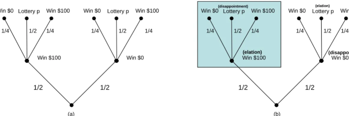
(elation) Lottery p 1/2 1/2 1/4 1/4 Win $100 Win $0 1/2 1/4 1/4 Lottery p Win $100 Win $0 1/2 Win $100 Win $0
(in addition to previously won $100)
(elation) (disappointment) (disappointment) Lottery p 1/2 1/2 1/4 1/4 Win $100 Win $0 1/2 1/4 1/4 Lottery p Win $100 Win $0 1/2 Win $100 Win $0
(in addition to previously won $100)
(a) (b)
Figure 2: Letpbe any lottery whose support consists of prizes between $25 and $3313. Then figure
(b) shows the only internally consistent history assignment for the three-stage lottery shown in (a),
usingβe=1,βd=2, andu(x) =x. The lotterypis a disappointment after first winning $100, and
an elation otherwise. Note that withu(x) =x, there cannot be any wealth effects on risk aversion.
5. Implications
In this section we discuss two phenomena that arise under HDDA, statistically cycling disappoint-ment attitudes and the possibility of “gray areas” where two DM’s, facing the same information
and having the same uandB, may disagree on which outcomes are elating or disappointing (the
history assignmenta) based on their optimistic or pessimistic tendencies. Further implications are
studied in Section 6, in a richer setting where intermediate actions may be taken while uncertainty resolves.
5.1. Disappointment cycles
Theorem 1 says that a DM with an HDDA representation overreacts to news. To illustrate the
implications of this, consider the three-stage lotteryP3shown in Figure 2(a). We assume u(x) =
x, βe =1, βd =2, and any choice of the other disappointment aversion coefficients satisfying
overreaction to news and the weak primacy effect.
Suppose that pis a lottery whose support consists of prizes between $25 and $3313. Then, the
two-stage sublotteryP`on the left—where the DM immediately accrues $100—must be elating in
P3, while the two-stage sublotteryPr on the right must be disappointing in P3. Indeed, this is the
only internally consistent history assignment because the worst outcome inP`dominates the best
outcome inPr. Therefore,P`is evaluated usingβe, andPr is evaluated usingβd.
Whether or not the DM wins $100, his additional winnings are determined by the same two-stage lottery,P=h14,δ0;12,p;14,δ100i. Becauseu(x) =x, there are no wealth effects: incrementing
all the prizes inPby 100 simply raises its HDDA utility by 100, without affecting which outcomes
are elating or disappointing. To calculate the value ofPusing HDDA, we fold it back by replacing
pwith its certainty equivalent calculated using the appropriate history assignment. Within each of
P` and Pr, we must determine whether p is an elation or a disappointment. Consider the lottery
h14,0;12,x;14,100ithat would result if pis replaced with a prizex. Using disappointment aversion,
it is easy to show that using βe =1, any prize x smaller than $3313 is a disappointment in this
lottery; while usingβd =2, any prizexlarger than $25 is an elation. But the certainty equivalent
of p, evaluated using any β, is always between $25 and $3313. Therefore, the only consistent
assignment ofpis as a disappointment after winning $100 and as an elation otherwise. That is, the
DM’s disappointment attitude must cycle, as shown in Figure 2(b).
This example suggests a more general prediction of HDDA. Note that in Gul (1991)’s original model, the disappointment aversion coefficient affects both risk aversion and the elation threshold.
Because the utility of the lottery determines its certainty equivalent, increasingβ lowers the DM’s
elation threshold: for any p∈L1 andβ0<β, if a prizexis (1) disappointing in punderβ then
it is disappointing in p under β0, and (2) elating in p under β0 then it is elating in p under β.
Because of this feature, overreaction to news means, in our dynamic setting, that a DM who has been elated is not only less risk averse than a DM who has been disappointed, but also has a higher elation threshold. In other words, overreaction to news implies that after a disappointment, the DM is more risk averse and “settles for less”; whereas after an elation, the DM is less risk averse
and “raises the bar.” As is in the example above, this leads tostatistically cycling disappointment
attitudes: disappointment is more likely after elation, and vice versa.
Under the assumption thatβh∈[βhe,βhd]for allh, HDDA implies condition (iii) in Proposition
1 (visualized in Figure 1). That condition says that after an elation, the DM’s greatest possible degree of risk aversion in the future decreases; and conversely, after a disappointment, the DM’s lowest possible degree of risk aversion in the future increases. However, in a finite horizon setting, this does not imply that the DM’s mood swings moderate in intensity with experience (for example, |βed−βe| ≥ |βede−βed| ≥ |βeded−βede| · · ·). That is, the intensity of disappointment cycles may
well persist.
5.2. Is the glass half full or half empty?
Consider the two stage lotteryhα,p; 1−α,δxiand suppose thatu(CEe(p))>u(x)>u(CEd(p)).
Under this assumption, it would be consistent for the lottery pto be either an elation or a
disap-pointment. The moral of this example is that while u, the collection B, and history assignmenta
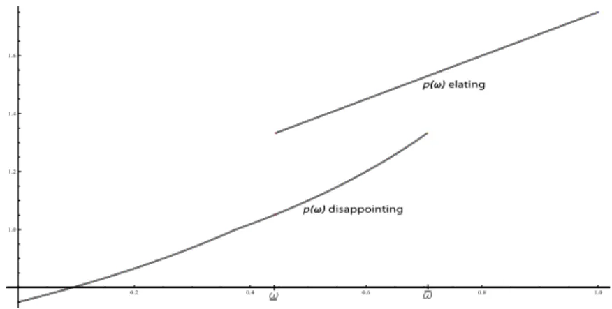
0.2 0.4 0.6 0.8 1.0 1.0 1.2 1.4 1.6 p() elating p() disappointing
Figure 3: The set of possible HDDA utilities of P(ω) are pictured on the vertical axis for each
ω∈(0,1)on the horizontal axis, givenβe=0,β0=1,βd=2, andu(x) =x. The sublotteryp(ω)
can be viewed as an elation or a disappointment in the range[ω,ω].
one cannot fully reconstruct the DM’s preference relation from only the information contained in
u and B. Predicting the DM’s behavior in such “gray areas” as above requires a theory of how
the DM assigns histories (as seen later, such a theory has testable predictions for his preference
relation overLT).
A dictionary definition of optimism is “An inclination to put the most favorable construction
upon actions and events or to anticipate the best possible outcome.”6 In our setting, optimism
and pessimism may be understood in terms of this multiplicity of internally consistent history assignments, where the optimist always chooses the most favorable one and the pessimist chooses the least favorable one.
Definition 4. We say that a DM is an optimist if for every PT ∈LT he chooses the sequential
and internally consistent history assignment a that maximizes his HDDA utility V(PT;u,a,B). Similarly, we say the DM is a pessimist if for every PT ∈ LT he chooses the sequential and
internally consistent assignmentathat minimizes his HDDA utilityV(PT;u,a,B). Given the same utility over prizes u and disappointment aversion coefficients B, we say that one DM is more optimistic than another if his HDDA utility is higher for everyPT ∈LT.
The optimist and pessimist agree on fundamentals (their utility from monetary prizes and their disappointment aversion coefficients), but they take a different perspective on what outcomes are disappointing and elating. This approach differs from most models of optimism and pessimism, which typically view optimism in terms of attaching higher probability to positive events. Under HDDA, probabilities are objective and unchanging, but endogenous reference dependence allows
the DM to select an internally consistent view of the unfolding risk according to his optimistic or pessimistic tendency.
To illustrate, consider Figure 3, which depicts for each ω ∈(0,1) all possible HDDA values
of the two-stage lotteryP(ω) =h13,δ1;13,δ2;13,p(ω)iwherep(w) =hω,3; 1−ω,0i. An increase
in ω is a first-order stochastic improvement of the risky sublottery p(ω). While p(ω)is
unam-biguously elating (disappointing) for high (low) values ofω, there is an intermediate range[ω,ω]
where p(ω)can be viewed either as an elation or as a disappointment. The certainty equivalents
of the other sublotteries are independent of their history assignment because they are degenerate.
At the same time, overreaction to news impliesCEe(p(ω))>CEd(p(ω)). Because HDDA utility
is increasing in the certainty equivalents, viewing p(ω)as an elation gives higher utility. The
op-timist thus views p(ω) as an elation as soon as possible (for all ω ≥ω). On the other hand, the
pessimist viewsp(ω)as a disappointment for as long as possible (for allω ≤ω). More generally,
a DM may have a cutoffω∗∈[ω,ω]at which p(ω)switches from a disappointment to an elation.
If one DM is more optimistic than another, then his cutoffω∗must be lower.
It is easy to see that overreaction to news implies that a DM with an HDDA representation
may violate first-order stochastic dominance on T-stage lotteries: for example, if the probability
α of pis very high, the lotteryhα,p; 1−α,δwi may be preferred tohα,p; 1−α,δbi; the “thrill
of winning” outweighs the “pain of losing.” The above example suggests, however, that both the optimist and pessimist satisfy the following regularity property related to first-order dominance,
stated for simplicity forT =2.
Proposition 2. Let be the preference relation represented by the DM’s HDDA utility on L2, and let>FOSDdenote the first-order stochastic dominance relation onL1. Fix any prizesx1, . . . ,xm−1
and probabilitiesα1, . . . ,αm. If the DM is an optimist or a pessimist, then7
hα1,δx1;. . .;αm−1,δxm−1;αm,pi hα1,δx1;. . .;αm−1,δxm−1;αm,qiwhenever p>FOSDq. (3)
The idea behind Proposition 2 is that fixing p as either an elation or a disappointment, the
utility ofP(ω)is increasing inω; and viewingpas an elation gives strictly higher utility for each
ω. The fact that the other sublotteries are degenerate ensures that the history assignment of p
does not affect their value. Consider instead a lotteryhα,p; 1−α,qi, where both p,q are risky
and p>FOSDq. Fixing anyβ, the certainty equivalent of pis larger than that of qby first-order
dominance; hence it would always be consistent to labelpas an elation andqas a disappointment.
7More generally, any DM whose history assignmentaapplies a cutoff for viewing the risky lottery as an elation (as in the above discussion) will also satisfy Property (3).
However, ifCEe(q)>CEd(p)then it would also be consistent to label pas a disappointment andq
as an elation; and if the probability 1−α ofqis sufficiently high, the optimist may achieve a higher
HDDA utility by doing so. The intuition is that by viewing a high probability, riskier prospect as an elation (if it is consistent to do so), the optimist puts a “positive spin” on the uncertainty. (A similar feature applies for the pessimist.)
6. HDDA with intermediate choices
We now extend the HDDA model to the setting of stochastic decision trees. Roughly speaking, a stochastic decision tree is a lottery over choice sets of shorter stochastic decision trees. In each
choice set, the DM can choose the continuation stochastic decision tree. Formally, for any setZ, let
K(Z)be the set of finite, nonempty subsets ofZ. A one-stage stochastic decision tree is simply a
one-stage lottery. The set of one-stage stochastic decision trees isD1=L1, with typical elements
p,q. For t =2, ..,T, the set of finite, nonempty sets of (t−1)-stage stochastic decision trees is
given by At−1 =K(Dt−1), with typical elements At−1,Bt−1. Then the set oft-stage stochastic
decision trees is the set of lotteries over finite choice sets of(t−1)-stage stochastic decision trees.
Formally, the set of t-stage stochastic decision trees is Dt =L(At−1), with typical elements
Pt,Qt. Our domain is thus DT =L(AT−1). (Our previous domain of T-stage lotteries can be
seen as the case in which all choice sets are degenerate.)
The realization of a t-stage stochastic decision tree is a choice set, which is categorized by
the DM as either elating or disappointing. The set of possible histories,H, is the same as before,
with the understanding that histories now refer to choice sets. We abuse notation and identify the
stochastic decision treePT ∈DT with a degenerate choice set, denotedAT :=
PT .
The folding back procedure may be extended to this richer domain in a way that the history assignment of a choice set determines the disappointment aversion coefficient applied to each stochastic decision tree inside it, and the value of the choice set itself is the maximal value of those stochastic decision trees. Formally, the certainty equivalent of each set of one-stage stochastic decision trees is determined by
uCEa(A1|PT)(A1)
=max
p∈A1V(p;u,βa(A1|PT)).
Fold back eachP2∈A2, by replacing each realization (a choice set,A1j) with its certainty
equiva-lent, as calculated above, to get the sublottery
fP2=hα1,CE
a(A1|PT)(A11);. . .;αm,CEa(A1
m|PT)(A
1
The certainty equivalent of a set of two-stage stochastic decision trees,A2,is determined by u CEa(A2|PT)(A2) = max n f P2:P2∈A2o V(fP2;u,β a(A2|PT)).
Continuing in this manner, the T-stage stochastic decision tree is reduced to a one-stage lottery
(over the certainty equivalents of its continuation subtrees) whose value is calculated using β0,
sincea(AT|PT) =0.
The definition of HDDA is almost the same as before.
Definition 5 (HDDA with intermediate choices). An HDDA utility representation overT-stage stochastic decision trees consists of an increasing and continuous utility over monetary prizes
u:X→R, a collection of disappointment aversion coefficientsB={βh}h∈H, and a history
assign-mentasatisfying, for eachPT ∈DT,
1. Sequential assignment. The DM assigns histories to all realizations of stochastic decision subtrees ofDT.Leta(AT|PT):=β0and, recursively, fort<T :
(i) ifPt+1is nondegenerate andAt∈suppPt+1∈At+1thena(At|PT)∈a(At+1|PT)×{e,d}.
(ii) ifPt+1is degenerate and andAt ∈suppPt+1∈At+1thena(At|PT) =a(At+1|PT).
2. Folding back. The DM calculates the utility of the stochastic decision tree by folding back. We letV(At;u,a,B|PT) andV(Pt;u,a,B|PT) denote, respectively, the value of any choice setAt inPT and subtreePt ofPT, as calculated above, simply writingV(PT;u,a,B)for the value ofPT.
3. Internal consistency. WithinPT, for each nondegeneratePt+1, ifAt∈suppPt+1is an elating (disappointing) outcome in Pt+1, then the value of At must be weakly larger than (strictly smaller than) the value ofPt+1inAT.
Observe that the DM is dynamically consistent under HDDA with intermediate actions. From any future choice set, the DM anticipates selecting the best stochastic decision tree. That choice leads to an internally consistent history assignment of that choice set. Thus, when reaching a choice set, the disappointment aversion coefficient she uses to value the choices therein is the one she anticipated using, and her choice is precisely her anticipated choice.
Internal consistency is therefore a stronger requirement than before, because it takes optimal choices into account. However, our previous results on the restrictions that internal consistency
imposes on how history affects disappointment aversion extend to the model of HDDA with inter-mediate actions.
Theorem 3 (Extension of previous results). The conclusions of Theorems 1 and 2 (necessary and sufficient conditions for HDDA) also hold for HDDA with intermediate actions.
6.1. Implications
Actions that can be taken while risk unfolds may arise naturally in various settings. Under HDDA, the DM’s risk taking behavior may depend on her history—she overreacts to news, and satisfies primacy effects. For example, overreaction to news suggests that a basketball player might attempt more difficult shots after a string of successful ones. Rao (2009), for example, finds evidence to this effect within the NBA, and uses this as an explanation for the “hot hand” fallacy, which is the
belief that a winning streak indicates future success (even in independent events).8
The biases predicted by HDDA, particularly the primacy effect, may also be exploited by agents who can manipulate the presentation of information to affect the DM’s behavior. For example, con-sider a financial advisor trying to sell a risky investment to a DM who has an HDDA representation
(u,a,B), with utility over monetary prizes u(x) =x and strictly positive disappointment aversion
coefficients ordered as in Figure 1. The risky investment, which requires an initial payment ofI, is
an even chance gamble betweenI+U andI−D. The DM knows that the upside,U, and downside,
D, are independently and uniformly distributed on{0,500,1000}. The financial advisor receives a
commission whenever the DM invests and is informed about the true values ofU andD. The DM
may consult with the financial advisor at no cost to learnU and D, and may choose whether or
not to invest based on the information provided. The financial advisor is obligated to tell the truth
aboutU andD, but can reveal this information in any order.9
It is straightforward to check that without any information, the DM prefers not to invest. Hence the DM chooses to consult with the advisor. Suppose the financial advisor has some good news and
some slightly worse news: the upside is high (U=1000) but the downside is moderate (D=500).10
How should she reveal this? Since the financial advisor knows the DM’s preferences, she can
8Unlike previous studies, such as Gilovich, Vallone and Tversky (1985), Rao controls for shot difficulty (i.e., taking more or less difficult shots after successes or failures) and shows that risk taking behavior —but not ability—is affected by previous outcomes.
9We assume for simplicity that the DM accepts the information the financial advisor gives in that order, without making inferences (this is an assumption often made in the context of framing effects); relaxing this assumption is interesting but beyond the scope of this example.
10This is the only case in which manipulation is possible. It is clear that when learningU=0, the DM would never invest; when learningD=0, the DM would always invest; and that the DM would not invest ifU=Dand he has strictly positive disappointment aversion coefficients.
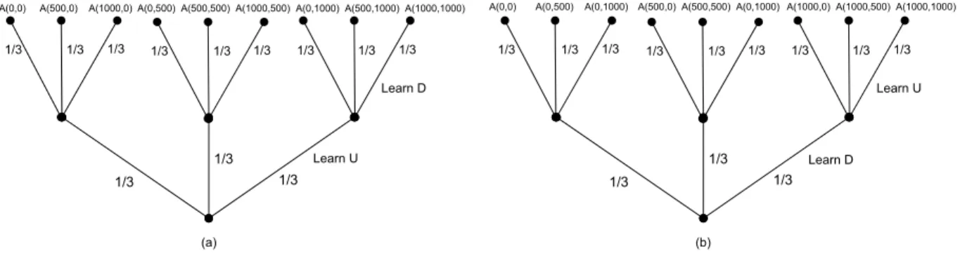
1/3 1/3 1/3 1/3 1/3 1/3 1/3 Learn U 1/3 1/3 1/3 1/3 1/3 Learn D 1/3 1/3 1/3 1/3 1/3 1/3 1/3 Learn D 1/3 1/3 1/3 1/3 1/3 Learn U (a) (b)
A(0,0) A(0,500) A(0,1000) A(500,0) A(500,500) A(0,1000) A(1000,0) A(1000,500) A(1000,1000) A(0,1000) A(500,1000) A(1000,1000)
A(0,500) A(500,500) A(1000,500) A(0,0) A(500,0) A(1000,0)
Figure 4: The stochastic decision tree that the DM faces when the financial advisor (a) reveals the upside first and the downside later or (b) reveals the downside first and the upside later. For given
U,D, the choice setA(D,U) ={δI,h.5,I+U;.5,I−Di}corresponds to either investing or not.
predict his choice based on how she provides information aboutU andD. ForU =1000 andD=
500, the DM will invest if the disappointment aversion coefficient used to evaluate the investment is smaller than one. The primacy effect suggests that conveying the best news first increases the DM’s inclination to invest. This can be formalized by applying HDDA to the stochastic decision
trees in Figure 4, which describe the DM’s problem when the financial advisor revealsU orDfirst.
For a wide range of disappointment aversion coefficients (for example, if βh∈[.5,1.5] for allh
andβed <1<βde), the DM is immediately disappointed whenD=500 is mentioned first, and
wouldn’t invest even upon hearingU=1000; while the DM is immediately elated whenU =1000
is mentioned first, and invests even upon hearingD=500. Therefore, the financial advisor should
reveal the best news first to minimize the DM’s subsequent risk aversion and ensure he invests.
7. Axiomatic foundations for HDDA on two-stage lotteries
In this section, we present axioms necessary and sufficient for a preference on the set of
two-stage lotteries, L2, to have an HDDA representation (with uniquely identifiedu, B, and history
assignmenta). This simplified setting allows for the clearest exposition of the underlying ideas;
we discuss the extension to more stages in Section 7.1.
For two-stage lotteries, an HDDA representation consists of an increasing and continuous
util-ity over prizesu:X →R, an internally consistent and sequential history assignmenta, and
dis-appointment aversion coefficientsB={β0,βe,βd}. The value of degenerate lottery P=h1,piis
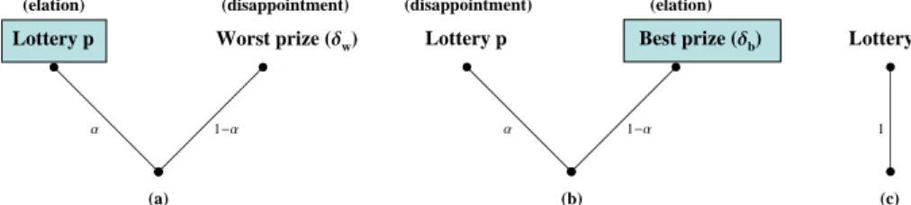
1-a a Lottery p (disappointment) (elation) Worst prize (dw) 1-a a Lottery p (disappointment) (elation)
Best prize (db) Lottery p
1
(a) (b) (c)
Figure 5: As the lottery pis varied, (a) corresponds to the objects inducing the relatione,α, (b)
corresponds tod,α; and (c) corresponds to0.
is given by V(P;u,a,B) = ∑{j|a(pj|P)=e}αju CEe(pj) + (1+β0)∑{j|a(pj|P)=d}αju CEd(pj) 1+β0∑{j|a(pj|P)=d}αj ,
where for eachh∈ {e,d},CEh(p)is the certainty equivalent of pcalculated using (1) withuand
βh. Recall further that internal consistency means, for example, that if p is elating in P (i.e.,
a(p|P) =e) then it should indeed be thatCEe(p)is weakly larger thanV(P;u,a,B).
In some two-stage lotteries, which history to assign to each realization can be determined by a quick inspection. For example, this is true of all the lotteries depicted in Figure 5. In the lottery in
Figure 5(b), which has the formhα,p; 1−α,δbi, receiving the lotterypis disappointing compared
to receiving the best monetary prize (b) with certainty.11 How should the DM compare the
two-stage lotteries P=hα,p; 1−α,δbi andQ=hα,q; 1−α,δbi, which both have this form? Both
pandqare disappointing in PandQ, respectively, and are received with the same probabilityα.
According to HDDA,βd must be applied to evaluate both pandqin the representation according
to disappointment aversion, and the value ofδbis fixed at u(b). Therefore, the preference overP
andQshould be determined by the utilities of pandqaccording to disappointment aversion, using
uandβd.
We define e,α on L1 by pe,α q if hα,δw; 1−α,pi hα,δw; 1−α,qi. Similarly, we
defined,α onL1bypd,α qifhα,δb; 1−α,pi hα,δb; 1−α,qiand0onL1byp0qif
h1,pi h1,qi. These relations are induced from preferences over the objects in Figure 5.
Our first axiom requires that these relations, induced from, each has a one-stage
disappoint-ment aversion representation. Axioms for one-stage disappointdisappoint-ment aversion are well-known and provided in Gul (1991).
11Except in the knife-edge case that p=
δb; however in that case the utility of the entire lottery isu(b)regardless of howpis labeled, and so not affecting Axiom DA.
Axiom DA (Disappointment aversion). The relations e,α, d,α, and 0 (induced from )
have a disappointment aversion representation with common utility over prizes u (up to affine
transformations).
As shown in Gul (1991), in any representation of the form (1),β is unique anduis unique up
to affine transformation. The requirement of a commonucaptures the idea that how risk unfolds
affects risk attitude through disappointment attitudes but not through the DM’s actual utility over
monetary prizes.12 Axiom DA does allow the disappointment aversion coefficients after each
history to differ.
Our next axiom says that “no news” does not affect the DM’s attitude toward risks. If he knows
that his monetary winnings will be determined by a one-stage lottery p, he does not care whether
the uncertainty in p is resolved now or later. Hence the DM’s risk attitude is not affected by the
mere passage of time, but rather only by previous disappointments and elations.
Axiom TN (Time neutrality).For all p∈L1,hp(x
1),δx1;p(x2),δx2;...;p(xm),δxni ∼ h1,pi. Recall that the procedure of folding back a two-stage lottery involves replacing each one-stage
lottery with its certainty equivalent. In HDDA, p is an elation inhα,δw; 1−α,pifor each α ∈
(0,1). We say that a prizexis anα-elation certainty equivalentofpif it solveshα,δw; 1−α,pi ∼
hα,δw; 1−α,δxi(theα-disappointment certainty equivalentis defined analogously). By Axiom
DA, it is clear that there exists a unique α-elation certainty equivalent for each p (and similarly
for disappointment). The next axiom says these certainty equivalents depend only on the history
assignment of p, independently of the probability with which it occurs.
Axiom CE (Uniform certainty equivalence). Take any p ∈ L1, x∈ X, and z∈ {w,b}. If
hα,δz; 1−α,pi ∼ hα,δz; 1−α,δxi for some α ∈(0,1), then hα0,δz; 1−α0,pi ∼ hα0,δz; 1−
α0,δxifor allα0∈(0,1).
We define CEe,(p), the elation certainty equivalent of p, as the value solving hα,δw; 1−
α,pi ∼ hα,δw; 1−α,δCEe,(p)ifor allα ∈(0,1). Thedisappointment certainty equivalentof p,
CEd,(p), is analogously defined.
12In particular, a behavioral implication of this assumption is that the DM’s Arrow-Pratt measures of risk aversion after each history are the same (see Gul (1991, Theorem 4)), assuming twice-differentiability ofu. Since we only know from the fact thatuis increasing on the bounded intervalXthat it is differentiable except on a measure-zero set, unchanginguimplies a constant relative marginal rate of substitution (MRS) condition where the derivatives exist. Our proof of the representation takes this route, showing that Axiom DA can be broken up into a requirement of disappointment aversion on each of these sets and such an MRS condition.
Recall that in the one-stage theory of disappointment aversion, each prize is categorized as an elating, neutral, or disappointing outcome; and if a prize is considered elating, for example, then it must be preferred to the lottery as a whole. In analogy, HDDA requires that if a one-stage lottery
pis elating in a two-stage lotteryP, then it must indeed be preferred toPas a whole. To study the
minimal departure that permits history dependence, HDDA assumes the certainty equivalent of a
lotterypinPis affected only by its assigned historyh(and therefore the same as calculated within
Lh(α)). This motivates the following definitions. Consider P=hα1,p1;. . .;αj,pj;. . . αm,pmi.
We say pjis elatinginPif
P∼ hα1,p1;. . .;αj,δCEe,(pj);. . . αm,pmi h1,δCEe,(pj)i.
Similarly, we say pjis disappointinginPif
P∼ hα1,p1;. . .;αj,δCEd,(pj);. . . αm,pmi h1,δCEd,(pj)i.
Our final axiom says that the preferencealways allows the DM to categorize a realizationpj
of a two-stage lotteryPaccording to one of the possibilities above.
Axiom CAT (Categorization). For any nondegenerate P∈L2 and any p∈suppP, p is either
elating or disappointing inP.
These axioms are equivalent to an HDDA representation on two-stage lotteries.
Theorem 4 (Representation). onL2 satisfies Axioms DA, TN, CE, and CAT if and only if it admits a history-dependent disappointment aversion (HDDA) representation with some contin-uous and increasing utility over monetary prizes u :X →R, history assignment a and a set of disappointment aversion coefficientsB={β0,βe,βd}.
In the theorem above, the disappointment aversion coefficients are unique; u is unique up to
positive affine transformation; and with endogenous reference dependence, the history assignment
is uniquely determined for eachP∈L2except in knife-edge cases that two decompositions would
givePthe same value.
7.1. Extending to three or more stages
With an appropriate modification of the axioms, Theorem 4 can be extended to represent
caseT =3; the more general case is similarly analyzed.
We must first generalize the sets of compound lotteries for which the history assignment of any final stage lottery, p, is unambiguous. For example, consider a lottery of the formhα,δ2w; 1−α,Pi,
wherePis of the formhα0,δb; 1−α0,pi. Here, the lottery pmust have the history assignmenth=
ed. We may define an induced preferenceed,(α,α0)onL1, and similarly for other possible history
assignments. Axiom DA requires that these induced preference relations have disappointment
aversion representations, and that the utility over prizesuis common (up to affine transformation)
in all these representations. The definition of the certainty equivalent of a sublottery is extended
analogously; for example, forh=ed,CEed(p)is the value solving
hα,δ2w; 1−α,hα0,δb,1−α0w2; 1−α,hα0,δb,1−α0,δCEed(p)ii
for allα,α0. Axiom CE then says that conditional on each history, the certainty equivalent of a
sublottery is independent of the probability with which it is received.
For any given single-stage lottery p, there are three compound lotteries in which the only
nondegenerate sublottery is the one where pis fully resolved. Axiom TN requires that the DM be
indifferent among these lotteries. Formally, for all p∈L1,
hp(x1),δ2x1;p(x2),δ2x2;...;p(xm),δ
2
xni ∼
h1,hp(x1),δx1;p(x2),δx2;...;p(xm),δxnii ∼ h1,h1,pii.
Lastly, Axiom CAT requires that a sublottery can be replaced by a degenerate lottery that gives the history dependent certainty equivalent of this sublottery for sure, with the consistency condition taking into account the history assignment of the sublottery. For example, if a one-stage lottery
p∈suppP=hα0,δb; 1−α0,piis replaced by its certainty equivalent after historyh=ed, then it
must be the case that
hα,δ2w; 1−α,Pi ∼ hα,δ2w; 1−α,hα0,δb,1−α0,δCEed(p)ii hα,δ
2
w; 1−α,δ
2
CEed(p)ii
8. Conclusion and directions for future research
We propose and axiomatize a model of history dependent disappointment aversion, in which risk attitudes depend endogenously on prior disappointments and elations. The HDDA model predicts that the DM satisfies two well-documented cognitive biases, overreaction to news and the primacy effect, as well as disappointment cycles; the DM raises the threshold for elation after positive
experiences but is willing to “settle for less” after negative ones, making disappointment more likely after elation and vice-versa.
To study endogenous reference dependence under the minimal departure from recursive appointment aversion, HDDA posits the categorization of each sublottery as either elating or dis-appointing. The DM’s risk attitudes depend on the prior sequence of disappointments or elations, but not on the “intensity” of those experiences. We are also interested in extending the HDDA model to permit such dependence. That extension raises several questions, beginning with how to define the intensity of elation or disappointment and how internal consistency is to be understood. The testable implications of such a model depend on whether it is possible to identify the extent to which a realization is disappointing, as that designation depends on the extent to which other options are elating or disappointing.
A. Appendix
A.1. Proofs for Section 4
Proof of Proposition 1. It is clear that (ii) implies (i), as both overreaction to news and the strong primacy effect respect the lexicographic ordering. Proving that (i) implies (ii) follows from alter-nating applications of overreaction to news and the strong primacy effect (with strict inequalities)
starting from the tail of the history. To illustrate, observe thatβeee<βeedby overreaction to news
withh=ee;βeed<βede by the strong primacy effect withh=e;βede<βedd by overreaction to
news withh=ed;βedd<βdee by the strong primacy effect withh=0; and so on and so forth.
Now assume thatβh∈[βhe,βhd] for allh. To see that (iii) implies (i), note that overreaction
to news is implied by takingh0=h00 =0; and that the strong primacy effect is implied by taking
h0=dtandh00=et. To see that (ii) implies (iii), observe that we knowβheh0<βhed|h0|andβhde|h00|<
βhdh00. Using the strong primacy effect to combine these bounds delivers the result if |h00|>|h0|;
so suppose that|h00|>|h0|(the other argument is symmetric). Then repeated use of the assumption
thatβhˆ ≤βhdˆ implies βhed|h0|≤βhed|h00|, and using the strong primacy effect again completes the proof. Lemma 1. IfTt τ=0(βedτ,βdeτ)6= /0, thenβedt+1 ≤βdet+1. Proof. Let Tt τ=0(βedτ,βdeτ) = β,β
. For each p∈L1 and
β ∈(−1,∞), define CEβ(p) = u−1(V(p;u,β)). Let
CEβ :=CEβ(h0.5,δw; 0.5,δbi)andCEβ :=CEβ(h0.5,δw; 0.5,δbi).
Let p be a lottery such that supp p⊂CE
β,CEβ
. Define P2 =hε,δw;ε,δb; 1−2ε,pi, P3=
hε,δ2w;ε,δ2b; 1−2ε,P2i, and continuing inductively,Pt+1=hε,δtw+1;ε,δtb+1; 1−2ε,Pti. That is,
in each stage 1, ...,t the lottery Pt+1 gives the worst and the best outcome, both with probability
ε and the continuation with the remaining probability. At periodt, the continuation lottery is the
lottery p. Note the following:
(i) For allβ,CEβ(p)⊂
CE
β,CEβ
. This is by monotonicity of the functional (1). (ii) Fixingβ,β0, limε→0V
hε,w;ε,b; 1−2ε,CEβ0(p)i;u,β
=V p;u,β0=u(CEβ0(p)).
(iii) For allτ, pis elating inP2=hε,δw;ε,δb; 1−2ε,piwhenP2is evaluated underβdeτ and p