6.851: Advanced Data Structures Spring Lecture 17 April 24

6.851: Advanced Data Structures Spring 2012

Lecture 17 — April 24

Prof. Erik Demaine Scribes: David Benjamin(2012), Lin Fei(2012),

Yuzhi Zheng(2012),Morteza Zadimoghaddam(2010), Sidd Seethepalli (2017), Diego Roque (2017), Aaron Bernstein(2007)

1

Overview

Up until now, we have mainly studied how to decrease the query time, and the preprocessing time of our data structures. The goal for this section is to use very “small” space. In this lecture, we will focus on maintaining the data as compactly as possible. Our goal will be to get as close the information theoretic optimum as possible, referred to as OPT. Note that most ”linear space” data structures we have seen are still far from the information theoretic optimum because they typically useO(n) words of space, whereas OPT usually uses O(n) bits. This strict space limitation makes it really hard to have dynamic data structures, so most space-efficient data structures are static. Here are some possible goals we can strive for:

• Implicit Data Structures – Space = OPT + O(1). Focusing on bits, not words. The ideal is to use OPT bits. The O(1) is there so that we can round up if OPT is fractional. Most implicit data structures just store some permutation of the data: that is all we can really do. As some simple examples, we can refer to heap which is a implicit dynamic data structure, and sorted array which is static example of these data structure.

• Succinct Data Structures– Space = OPT +o(OPT). In other words, the leading constant is 1. This is the most common type of space-efficient data structure.

• Compact Data Structures– Space =O(OPT). Note that some ”linear space” data structures are not actually compact because they useO(w·OPT) bits. This saves at least anO(w) factor compared to normal data structures. For example, suffix trees use O(n) words of space, but the information theoretic lower bound is n bits. On the other hand, BST can be seen as a compact data structure.

Succinct is the usual goal here. Implicit is very hard, and compact is generally to work towards a succinct data structure.

1.1 Mini-survey

• Implicit Dynamic Search Tree – Static search trees can be stored in an array with lnn per search. However, supporting inserts and deletes makes the problem more tricky. There is an old result that was done in log2n using pointers and permutation of the bits. In 2003, Franceschini and Grossi [1] developed an implicitly dynamic search tree which supports insert, delete, and predecessor inO(logn) time worst case, while also being cache-oblivious.

• Succinct Dictionary – This is static, which has no inserts and deletes. In a universe of size u, there are u_n

ways to have n items, so the information theoretic lower bound is log u_n bits. There are results using log _nu

+O log( u n) log log logu

bits [2] or log u_n

+O(n(log log_lognn)2) bits [6], which supportO(1) membership queries, which is the same runtime but with less space than normal dictionaries.

• Succinct Binary Tries– The number of possible binary tries withnnodes is thenth Catalan number,Cn= _2n1₊₁ 2_nn

≈4n. Thus, OP T ≈log(4n) = 2n. We note that this can be derived from a recursion based on the sizes of the left and right subtrees of the root. In this lecture, we will show how to use 2n+o(n) bits of space. We will be able to find the left child, the right child, and the parent in O(1) time. We will also give some intuition for how to answer subtree-size queries inO(1) time. Subtree size is important because it allows us to keep track of the rank of the node we are at. Motivation behind the research was to fit the Oxford dictionary onto a CD, where space was limited.

• Almost Succinct k-ary trie – The number of such tries is C_nk = _kn1₊₁ kn_n+1

≈ 2(logk+loge)n. Thus, OPT = (logk+ loge)n. The best known data structures was developed by Benoit et al. [3]. It uses (dlogke+dlogee)n+o(n) +O(log logk) bits. This representation still supports the following queries inO(1) time: find child with labeli, find parent, and find subtree size.

• Succinct Rooted Ordered Trees– These are different from tries because there can be no absent children. The number of possible trees isCn, so OPT = 2n. A query can ask us to find the

ith child of a node, the parent of a node, or the subtree size of a node. Clark and Munro [4] gave a succinct data structure which uses 2n+o(n) space, and answers queries in constant time.

• Succinct Permutation– In this data structure, we are given a permutationπ ofnitems, and the queries are of the formπk(i). Munro et. al. present a data structure with constant query time and space (1 +)nlog(n) +O(1) bits in [7]. They also obtain a succinct data structure withdlogn!e+o(n) bits and query timeO(_{log log}logn_n).

• Compact Abelian groups – Represent abelian group onn items using O(logn) bits, and rep-resent an item in that list with lognbits.

• Graphs– More complicated. We did not go over any details in class.

• Integers – Implicit n-bit number of integers can do increment or decrement in O(logn) bits reads and O(1) bit writes.

OPEN: O(1) word operations.

2

Level Order Representation of Binary Tries

As noted above, the information theoretic optimum size for a binary trie is 2n bits, two bits per node. To build a succinct binary trie, we must represent the structure of the trie in 2n+o(n) bits. We represent tries using thelevel order representation. Visit the nodes in level order (that is, level by level starting from the top, left-to-right within a level), writing out two bits for each node. Each bit describes a child of the node: if it has a left child, the first bit is 1, otherwise 0. Likewise, the second bit represents whether it has a right child.

As an example, consider the following trie:

We traverse the nodes in order A, B, C, D, E, F, G. This results in the bit string: 11 01 11 01 00 00 00

A B C D E F G

External node formulation Equivalently, we can associate each bit with the child, as opposed to the parent. For every missing leaf, we add an external node, represented by · in the above diagram. The original nodes are called internal nodes. We again visit each node in level order, adding 1 for internal nodes and 0 for external nodes. A tree with nnodes has n+ 1 missing leaves, so this results in 2n+ 1 bits. For the above example, this results in the following bit string:

1 1 1 0 1 1 1 0 1 0 0 0 0 0 0 A B C · D E F · G · · · ·

Note this new bit string is identical to the previous but for an extra 1 prepended for the root, A.

2.1 Navigating

This representation allows us to compute left child, right child, and parent in constant. It does not, however, allow computing subtree size. We begin by proving the the following theorem:

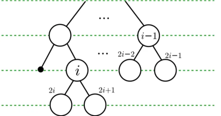
Theorem 1. In the external node formulation, the left and right children of the ith internal node are at positions 2iand 2i+ 1.

Proof. We prove this by induction on i.

For i= 1, the root, this is clearly true. The first entry of the bit string is for the root. Then bits 2i= 2 and 2i+ 1 = 3 are the children of the root.

Now, fori >1, by the inductive hypothesis, the children of thei−1st internal node are at positions 2(i−1) = 2i−2 and 2(i−1) + 1 = 2i−1. We show that the children of theith internal immediately follow thei−1st internal node’s children.

Visually, there are two cases: either i−1 is on the same level as ioriis on the next level. In the second case,i−1 andiare the last and first internal nodes in their levels, respectively.

Figure 1: i−1 andiare on the same level.

Figure 2: i−1 andi are different levels.

Level ordering is preserved in children, that is,A’s children precedeB’s children in the level ordering if and only ifA precedes B. All nodes between the i−1st internal node and theith internal node are external nodes with no children, so the children of theith internal node immediately follow the children of thei−1st internal node, at positions 2iand 2i+ 1.

As a corollary, the parent ofbit position iisb₂ic. Note that we have two methods of counting bits: we may either count bit positions or rank only by 1s. If we could translate between the two inO(1) time, we could navigate the tree efficiently.

3

Rank and Select

Now we need to establish a correspondence between positions in the n-bit string and actual internal node number in the binary tree.

Say that we could support the following operations on an n-bit string in O(1) time, with o(n) extra space:

• rank(i) = number of 1’s at or before position i

• select(j) = position ofjth one

This would give us the desired representation of the binary trie. The space requirement would be 2n for the level-order representation, and o(n) space for rank/select. Here is how we would support queries:

• left-child = 2 rank(i)

• right-child = 2 rank(i) + 1

• parent(i) = select(₂i)

Note that level-ordered trees do not support queries such as subtree-size. This can be done in the balanced parentheses representation, however.

3.1 Rank

This algorithm was developed by Jacobsen, in 1989 [5]. It uses many of the same ideas as RMQ. The basic idea is that we use a constant number of recursions until we get down to sub-problems of sizek= log(₂n). Note that there are only 2k=√npossible strings of size k, so we will just store a lookup table forall possible bit strings of size k. For each such string we havek=O(logn) possible queries, and it takes log(k) bits to store the solution of each query (the rank of that element). Nonetheless, this is still onlyO(2k·klogk) =O(√nlognlog logn) =o(n) bits.

Notice that a naive division of the entire n-bit string into chunks of size 1₂logn does not work. because we need to save _logn_n relative indices, each taking up to lognbits, for a total of Θ(n) bits, which is too much. Thus, we need to use a technique that uses indirection twice.

Step 1: We build a lookup table for bit strings of length 1₂logn. As we argued before, this takes O(√nlognlog logn) =o(n) bits of space.

Step 2: Split the the n-bit string into (log2n)-bit chunks.

At the end of each chunk, we store the cumulative rank so far. Each cumulative rank would take lognbits. And there are at most n

log2n chunks. Thus, the total space required isO n log2nlogn = O_logn_nbits.

Step 3: Now we need to split each chunk into 1₂logn-bit sub-chunks.

Then, at the end of each sub-chunk, we store the cumulative rankwithin each chunk. Since each chunk only has size log2n, we only need log logn bits for each index. There are at mostO_logn_n sub-chunks. Thus, the total space required isO_logn_nlog logn=o(n) bits. Notice how we saved space because the size of the cumulative rank within each small chunk is less.

OJAQELW

FKXQNV VWRUHFXPXODWLYHUDQNOJQELWV

OJQELW

VXEFKXQNV VWRUHFXPXODWLYHUDQNZLWKLQFKXQNOJOJQELWV

Figure 3: Division of bit string into chunks and sub-chunks, as in the rank algorithm

Step 4: To find the total rank, we just do:

Rank = rank of chunk + relative rank of sub-chunk within chunk + relative rank of element within sub-chunk (via lookup table).

This algorithm runs in O(1) time, and it only takes O(nlog log_lognn) bits. It is in fact possible to improve the space to O n

logk_n

bits for any constant k. But this is not covered in class.

3.2 Select

This algorithm was developed by Clark and Munro in 1996 [4]. Select is similar to rank, although more complicated. This time, since we are trying to find the position of the ith one, we will break our array up into chunks with equal amounts of ones, as opposed to chunks of equal size.

Step 1: First, we will pick every (lognlog logn)th 1 to be a special one. We will store the index of every special one. Storing an index takes lognbits, so this will take O

n_lognlog_{log log}n _n = O n log logn =o(n).

Then, given a query, we can find divide it by lognlog logn to teleport to the correct chunk con-taining our desired result.

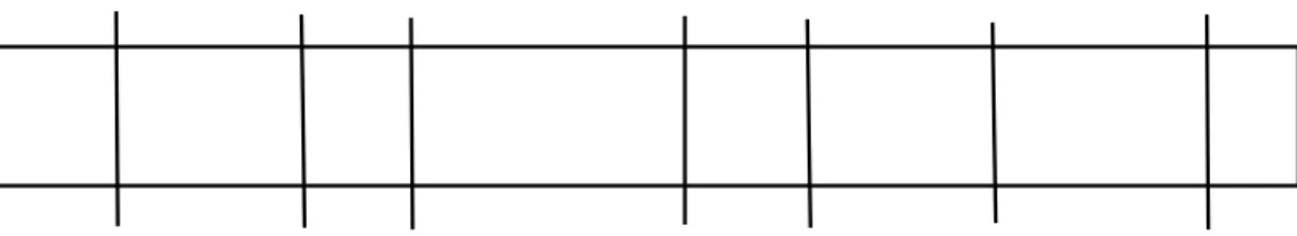
Step 2: Now, we need to restrict our attention to a single chunk, which contains lognlog logn 1 bit. Let r be thetotal number of bits in a chunk.

XQHYHQGLYLVLRQRIELWVWULQJHDFKFRQWDLQLQJHDFWO\OJQOJOJQV

Figure 4: Division of bit string into uneven chunks each containing the same number of 1’s, as in the select algorithm

This is when the 1 bits are sparse. Thus, we can afford to store an array of indices of every 1 bit in this chunk. There are (lognlog logn) 1 bits. Storing each would take up at most lognspace (The size of the chunk is already polylog(n), so lognbits is more than enough). And there are at most

n

(lognlog logn)2 such sparse chunks. So, in total, we use space (in bits):

O

n

(lognlog logn)2(lognlog logn) logn =o n log logn .

Case 2: Ifr ≤(lognlog logn)2 bits:

We have reduced to a bit string of length r≤(lognlog logn)2. This is good, because analogously to Rank, these chunks are small enough to be divided into sub-chunks without requiring too much space for storing the sub-chunk’s relative indices.

Step 3: We basically repeat steps 1 and 2 on all reduced bit strings, and further reduce them into bit strings of length (log logn)O(1).

Step 1’:

With the reduced chunks of lengthO(lognlog logn)2, we again pick out special 1’s, and divide it into every (log logn)2th 1 bit. Since within each chunk, the relative index only takes O(log logn) bits, the total space (in bits) required is:

O

n

(log logn)2 log logn =O n log logn Step 2’:

Within groups of (log logn)2 1 bits, say it has r bits total: Case 1: Ifr ≥(log logn)4:

Store relative indices of 1 bits. There are _{(log log}n _n)4 such groups, within each there are (log logn)2

1 bits, and each relative index takes log lognbits to store. For a total of: O(_{(log log}n _n)4(log logn)2log logn) =O(_{log log}n _n) bits.

Case 2: Ifr ≤(log logn)4: We have r≤ 1

2logn. Then it is small enough for us to use step 4: Step 4:

Use a lookup table for bit string of length ≤ 1₂logn. Like in rank, the total space for the lookup table is at most:

O(√nlognlog logn).

Thus, we again haveO(1) query time andO(_{log log}n _n) bits space. Again, this result can be improved to O

n logk_n

bits for any constant k, but we will not show it here.

4

Subtree Sizes

We have shown a Succinct binary trie which allows us to find left children, right children, and parents. But we would still like to find sub-tree size in O(1) time. Level order representation does not work for this, because level order gives no information about depth. Thus, we will instead try to encode our nodes in depth first order.

In order to do this, notice that there are Cn (catalan number) binary tries on n nodes. But there are also Cn rooted ordered trees on n nodes, and there are Cn balanced parentheses strings with n parentheses. Moreover, we will describe a bijection: binary tries ⇔ rooted ordered trees ⇔

balanced parentheses. This makes the problem much easier because we can work with balanced parentheses, which have a natural bit encoding: 1 for an open parentheses, 0 for a closed one.

4.1 The Bijections $ % & ' ( ) *

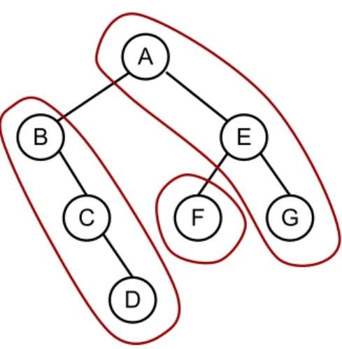
Figure 5: An example binary trie with circled right spine.

node lives in a spine. To make this into a rooted ordered tree, we can think of rotating the trie 45 degrees counter-clockwise. Thus, the top three nodes of the tree will be the right spine of the trie (A,C,F). To make the tree rooted, we will add an extra root *.

Now, we recurse into the left subtrees of A,C, and F. For A, the right spine is just B,D,G. For C, the right spine is just E: C’s only left child. Figure 6 shows the resulting rooted ordered tree. There is a bijection between the two representations.

$ % & ' ( ) *

Figure 6: A Rooted Ordered Tree That Represents the Trie in Figure 5.

To go from rooted ordered trees to balanced parentheses strings, we do a DFS (or Euler tour) of the ordered tree. We will then put an open parentheses when we first touch a node, and then a closed parentheses the second time we touch it. Figure 7 contains a parentheses representation of the ordered tree in Figure 2.

( ( ( ) ( ) ( ) ) ( ( ) ) ( ) ) * A B B C C D D A E F F G G E *

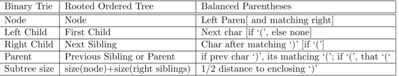
Figure 7: A Balanced Parentheses String That Represents the Ordered Tree in Figure 6 Now, we will show how the queries are transformed by this bijection. For example, if we want to find the parent in our binary trie, what does this correspond to in the parentheses string? he bold-face is what we have in the binary trie, and under that, we will describe the corresponding queries from the 2 bijections.

Binary Trie Rooted Ordered Tree Balanced Parentheses

Node Node Left Paren[ and matching right]

Left Child First Child Next char [if ‘(’, else none] Right Child Next Sibling Char after matching ‘)’ [if ‘(’]

Parent Previous Sibling or Parent if prev char ‘)’, its mathcing ‘(’; if ‘(’, that ‘(‘ Subtree size size(node)+size(right siblings) 1/2 distance to enclosing ‘)’

Could use rank and select to find the matching parenthesis for the balanced parenthesis represen-tation.

References

[1] G. Franseschini, R.Grossi Optimal Worst-case Operations for Implicit Cache-Oblivious Search Trees, Prooceding of the 8th International Workshop on Algorithms and Data Structures (WADS), 114-126, 2003

[2] A.Brodnik, I.Munro Membership in Constant Time and Almost Minimum Space, Siam J. Computing, 28(5): 1627-1640, 1999

[3] D.Benoit, E.Demaine, I.Munro, R.Raman, V.Raman, S.RaoRepresenting Trees of Higher De-gree, Algorithmica 43(4): 275-292, 2005

[4] D.Clark, I.Munro Eifficent Suffix Trees on Secondary Storage, SODA, 383-391, 1996.

[5] G.JacobsonSuccinct Static Data Structures, PHD.Thesis, Carnegie Mellon University, 1989. [6] R. Pagh: Low Redundancy in Static Dictionaries with Constant Query Time, SIAM Journal

of Computing 31(2): 353-363 (2001).

[7] J. Ian Munro, Rajeev Raman, Venkatesh Raman, and Satti Srinivasa Rao: Succinct Represen-tations of PermuRepresen-tations, ICALP (2003), LNCS 2719, pp. 345-356.