Urbschat, Florian und Watzka, Sebastian:
Quantitative Easing in the Euro Area
Munich Discussion Paper No. 2017-10
Department of Economics
University of Munich
Volkswirtschaftliche Fakultät
Ludwig-Maximilians-Universität München
Quantitative Easing in the Euro Area
-An Event Study Approach
Florian
Urbschat
Sebastian
Watzka
University of Munich
Hans-Böckler-Foundation
Seminar for Macroeconomics Macroeconomic Policy Institute (IMK)
Abstract
We examine the effects of the Asset Purchase Programme (APP) gradually introduced by the European Central Bank from September 2014 onwards. Studying the short-term reaction of financial markets after APP press releases, we analyse the development of bond yields and spreads around these releases. More precisely, we try to estimate different asset price channels by quantifying the cumulative decrease of spreads and by running event regressions for several Euro Area countries. Focusing on the signalling channel, measured by the OIS rate, and the portfolio rebalancing channel, proxied by the conditional bond-OIS spread, we find that the effects in yield and spread reduction were most pronounced for the initial announcement on the Public Sector Purchase Programme (PSPP) but declined afterwards for additional announcements. Possible explanations for this are the declining degree to which the ECB surprised markets and the increasingly burdensome institutional set-up of the APP. While yield reductions were larger for periphery countries’ than for core countries’ bonds, our evidence suggests that this stronger reduction is mostly due to a decreasing risk component of southern bonds. In fact, once controlling for this implicit credit risk reduction we find rather mild effects from portfolio rebalancing for all countries.
JEL Codes: E43, E44, E52, E58, G14
Keywords: Large Scale Asset Purchase, Yield curve, Quantitative Easing, APP, Event study.
Acknowledgements: We are thankful to Gerhard Illing, Paul de Grauwe, Markus Brunnermeier, Klaus Adam, Michael Weber, and Guglielmo Caporale for valuable advice. We also appreciate helpful comments and suggestions by the partic-ipants of the CESifo Macro, Money & International Finance Conference 2017, the EEA 2017 Lisbon Conference, the VfS Annual Conference 2017, the Belgrade Young Economist Conference, the RGS Econ 10TH Doctoral Conference, and the Macroeconomics Seminar at the University of Munich. Finally, we acknowledge research assistance by David Gramke and Patrick Weiß. Any remaining errors are the responsibility of the authors. Corresponding author: Florian Urbschat
1
Introduction
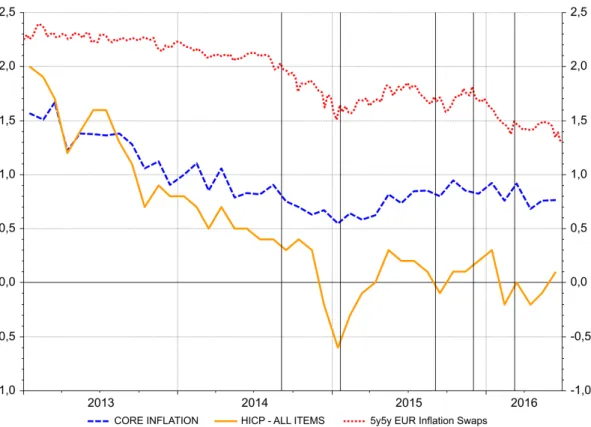
After a severe drop in inflation rates and medium-term inflation expectations during 2014, the Eu-ropean Central Bank gradually introduced the Asset Purchase Programme (APP) with a total monthly purchase volume of between 60 and 80 billion EUR1. In fact, headline inflation plunged to −0.6% in January 2015, with core inflation, excluding more volatile goods such as oil or energy prices, showing a clear downward trend since 2013 as outlined in figure 1. Even more importantly, the 5y5y inflation forward swaps, the ECB’s preferred measure of medium term inflation expectation, started declining in 2014, threatening inflation expectations becoming de-anchored. Being in danger of missing its inflation target in the medium-run, the ECB gradually introduced the APP and consequently emphasized that the ultimate aim of this quantitative easing (QE) programme is to fulfil its mandate of maintaining price stability. Accordingly, the ECB officially stated that “(the Asset Purchase Programme) will help to bring inflation back to levels in line with the ECB’s objective”2.
Comparing the ECB’s policy to other major central banks like the Fed or the Bank of England, both of these institutions have introduced various conventional and unconventional monetary policy measures during the global financial crisis of 2008-09, including large QE programmes. Whereas these central banks purchased domestic government bonds on a large scale early on, the ECB during the financial crisis rather focused on buying covered bonds and provided exceptional liquidity measures to banks3. Because some member countries in the Euro Area were worried about potentially strong effects on inflation, other unintended consequences, or the compatibility of a QE programme with European law, the European Central Bank avoided large purchases of government bonds during the initial phase of the financial and European debt crisis.
The early stage of unconventional monetary policy measures after 2008 has been studied intensively in the literature. Three main conclusions can be drawn: First, the strongest reaction of finanical mar-kets is expected to occur upon announcement of the stock of pruchases, while the effects from the actual execution of the programme are minor in comparison. These two effects are often referred to as “stock” versus “flow” effects. Second, among several possible channels proposed by the literature “narrow chan-nels” (targeting just a few asset) usually seem to have stronger effects compared to “broader chanchan-nels” (aiming to effect also other market segments via spill-over effects). Finally, asset purchase programmes that were conducted in times of stressed markets and high uncertainty seem to have a stronger impact
than programmes that were announced when market conditions were relaxed4. In this respect, it is
important to note that the European Central Bank started its QE programme in times when financial markets were relatively calm suggesting rather minor effects from it.
1
The initial size of 60 billion EUR per month was increased to 80 billion EUR in March 2016 and lowered again to 60 billion EUR in December 2016. See section2and section5for details.
2
Seehttps://www.ecb.europa.eu/explainers/tell-me-more/html/asset-purchase.en.html. 3
These encompassed three-year loans to eligible banks, unlimited liquidity provisions via a fixed-rate full-allotment procedure, or lowering the deposit rate to zero. Only after the outbreak of the European debt crisis the ECB started to purchase government bonds in 2010 under the Securities Markets Programme (SMP). However, the SMP is usually not regarded as a full blown QE programme.
4
Figure 1: Headline and Core Inflation in the Euro Area
Source: Datastream. Vertical lines indicate APP announcements.
As it remains too early to judge the wider impact of the APP on macroeconomic conditions in the Euro Area, this paper examines if the ECB has been successful in achieving the intermediate goal of lowering long-term bond yields. Reducing these yields should flatten the yield curve, lead to more credit to the real sector, increase aggregate demand, and ultimately also increase inflation. To find some first evidence whether this necessary pre-condition has been achieved, we use an event study methodology to examine the effects of APP press releases on bond yields. More precisely, we systematically search for key ECB policy announcements and consider how selected Euro Area bond yields were affected by different asset price channels. Most importantly, we examine how the conditional bond-OIS spread, a proxy for the effect of portfolio rebalancing5, changed during our events.
Our analysis suggests that the ECB’s policy had strong and desired effects on financial markets at the very beginning, but less so subsequently. As a result of the portfolio rebalancing channel and a potential reduction in credit and liquidity risk premia, we estimate a cumulative reduction in yields of Euro Area government bonds ranging from 85.80 basis points (BPS) for Portugal to only 5.91 BPS for
5
Under the assumption that assets are not perfect substitutesTobin (1969), among others, argued that a change in the relative supply of a specific asset, e.g. due to an intervention by the central bank, must result in a change in the relative expected return of the asset, all else equal. Suppose the QE policy of the central bank leads to a rise in the price for a long-term government bond and, hence, to a drop in the expected return of an investor’s portfolio. Keeping the desired expected return of her portfolio constant, the investor now needs to buy other assets with broadly similar characteristics in terms of risk or maturity to maintain the overall expected return of her portfolio. Thus, via therebalancing of investors’ portfolios the price and yield of other assets are also changing.
Germany. In our view, possible explanations for such mild effects for some Euro Area countries are the timing of the APP and the strict self-imposed regulations by the ECB. Notably, the ECB decision to not buy bonds trading below the deposit facility could potentially dampen positive effects from the APP6. In contrast, the much stronger reductions for periphery countries like Portugal or Italy suggest that markets implicitly also lowered the risk premia for these countries. Put differently, countries with a higher yield reacted stronger to APP announcements compared to countries having a low yield already near the zero lower bound.
The remainder of this paper is organized as follows. Section2describes some important institutional details of the ECB’s QE programme. Section3reviews the large and growing literature on different QE programmes and their success so far. Section 4 describes the theoretical considerations for measuring the portfolio rebalancing channel by the bond-OIS spread. Section5outlines the data set in detail with special focus on identifying event dates. Next, the reaction of bond markets is presented in section 6 followed by event regressions in section7. Section8concludes.
2
APP Institutional Details
Due to the incomplete integration of the current monetary union of the Euro Area the Asset Purchase Programme conducted by the ECB has some important regulations and characteristics with respect to its design. As we will argue, some of these regulations may seriously dampen the desired effects of the APP.
To begin with, the APP is actually an umbrella term for four different purchase programmes: the Third Covered Bond Purchase Programme (CBPP3), the Asset Backed Securities Purchase Programme (ABSPP), the Public Sector Purchase Programme (PSPP), and the Corporate Sector Purchase Pro-gramme (CSPP). In total, the ECB’s asset purchases under the APP have a target rate of 60 to 80
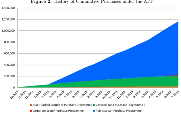
billion EUR per month, which accumulated to 1,084,583 million EUR in June 2016. Table 1
summa-rizes the main features of each programme while figure2illustrates the cumulative purchases over time, indicating that the in terms of scale the PSPP is by far the largest.
Even though the programmes differ considerably by size and scope they also share some common features. First of all, all APP programmes are in principal open-ended and are intended to continue until the ECB sees the inflation rate back on track on a sustained inflation path in line with the ECB’s target rate of close to but below2%. As a benchmark the APP was initially intended to last at least until September 2016, which has already been extended twice, first, to March 2017 and, a second time, to December 2017.
Secondly, important aspects to notice are the regulations concerning hypothetical losses from the ECB’s asset purchases. Unlike a national central bank the ECB is not owned by a national government
6
In fact, the ECB has eased this constraint in the Monetary Policy Decision of December 2016 by stating that under the APP purchases with a yield below the deposit facility “will be permitted to the extent necessary”. See
but by all the National Central Banks from each member state. Taking into account this unique institu-tional structure of the Euro Area, the majority of the asset purchases are conducted in the home market of each National Central Bank according to its respective capital share in the ECB. Subsequently, in case of a hypothetical default of e.g. a single Portuguese government bond bought by the Banco de Portugal, only the Banco de Portugal would incur the respective loss for this bond7. Note, however, a smaller part of asset purchases of about 20% are conducted directly by the ECB. Hypothetical losses to these purchases are subject to loss sharing.
Table 1: Asset Purchase Programme Overview
Programme Monthly Net Purchases Total Holdings In Percent Start of Programme
CBPP3 3,258 183,377 16.02 October 2014
ABSPP 854 19,607 1.75 November 2014
PSPP 69,658 875,201 81.09 March 2015
CSPP 6,816 6,398 1.13 June 2016
Source: ECB; holdings at amortized cost, in million EUR, at month end.
Figure 2: History of Cumulative Purchases under the APP
0 200,000 400,000 600,000 800,000 1,000,000 1,200,000 1,400,000
Asset-Backed Securities Purchase Programme Covered Bond Purchase Programme 3 Corporate Sector Purchase Programme Public Sector Purchase Programme
Source: ECB; holdings at amortized cost, in million EUR, at month end.
Since the PSPP is by far the largest programme it is the main focus of this paper. As the intended goal of the programme is to lower long-term government bond yields, the ECB initially intended to buy only mid- and longer-term bonds with a remaining maturity of 2 to 30 years8. Yet, not all bonds bought by the ECB are government bonds. In fact, roughly10%of bonds purchased are international organizations
7
Given no other National Central Bank bought the same bond. 8
and multilateral development banks such as the EU or the European Investment Bank. Also, there is a long list of regional governments or recognized government institutions, such as the German KfW or the French Caisse, which are eligible for the bond buying programme9. As already indicated the issue of collective liability and risk sharing is sensitive in the case of the ECB. Therefore, in order to avoid potential trade-offs in case of default, the ECB initially only bought bonds up to 33% per issuer and 25%per issue of a single bond, the idea being not to have a blocking minority in collective action clause assemblies. To increase flexibility, this rule was gradually increased to33% per issue for public entities, subject to a case-by-case verification, and 50%of issuer and issue share for international organizations and multilateral development banks. Since the ECB does not publish a full list of bonds (and respective shares) bought, it remains unclear how strong this constraint might tightened the hands of the ECB10.
Additionally, another aspect jeopardizing a successful implementation of the PSPP is the current negative interest and yield environment. In order to avoid large losses from bond purchases, the ECB vowed to a self-imposed regulation of not buying bonds trading at a yield below the deposit facility rate. The ECB was the first large central bank to introduce negative interest rates by lowering the deposit facility to −0.1% in June 2014. Afterwards, the deposit facility has been lowered gradually
down to −0.4% in March 2016. For details see figure 11 and 12 in the Appendix. As we will see in
section 5, under this constraint a large and increasing number of bonds are not eligible for the APP programme11. We will argue that these tight self-imposed regulations seriously constrain the ECB in a successful implementation of their QE programme especially for Euro Area core countries.
3
Literature Review
A very large and continuously growing literature exists on the effects of quantitative easing pro-grammes. Since the start of the first QE programme by the Bank of Japan in 2001 the topic raised increasing academic attention (see for instanceUgai (2006)for an early empiric assessment). However, the number of academic papers exploded after the financial crisis of 2008-09 when the US Fed, the Bank of England, the Bank of Japan, or the European Central Bank all started various kinds of asset purchas-ing or unconventional monetary policy measures. A strict categorization of different approaches in the literature is obviously difficult. Nevertheless, let us try to loosely group the literature into three different groups of papers: theoretical, long-term empirical and short-term empirical.
A first stream of literature considers how large asset purchasing programs can be built into standard
New Keynesian models, which mostly suggest the irrelevance of such a policy as in Eggertsson and
Woodford (2003)12. One such approach can be found in Cúrdia and Woodford (2011). Generalising
9
Also note that ECB currently does not purchase any Greek government bonds. 10
Some authors predicated that the ECB could hit these limits for e.g. German Bunds around March 2017 (see for instance Claeys, A. Leandro, et al. (2015)). Yet, this early assessment does not included later changes to policies as mentioned above. More recent studies, such asClaeys and L. Leandro (2016), suggested that purchases of German bonds will be constraint between April 2017 and March 2018. However, in December 2016 the ECB announced that purchases for bonds below the deposit facility “will be permitted to the extent necessary”, which again relaxes this constraint.
11
See also figure4. 12
the findings of Eggertsson and Woodford (2003), the authors show that targeted asset purchases can be effective if financial markets are sufficiently disrupted, i.e. if private-sector financial intermediation is inefficient. However, QE can still be irrelevant if the central bank conducts pure quantitative easing (buying Treasury securities) rather than credit easing (lending directly to the private sector), or if the central bank cannot change people’s believe about the future interest rate policy. A second approach is the limitation of arbitrage, often modelled by assuming some kind of segmented asset markets, e.g.
due to preferred-habitat motives as in Vayanos and Vila (2009). One example is Chen et al. (2012)
where the authors aim to simulate the second Large Scale Asset Purchase (LASP) programme by the Fed, by augmenting a standard DSGE model (with nominal and real rigidities) with segmented bond markets. According to the authors, their paper “wants to give LSAP programs a chance” [Chen et al. (2012), p. 290] by assuming that heterogeneous preferences for assets of different maturities exist leading to such kind of asset market segmentation. This implies that the long-term interest rate plays a role in determining aggregate demand distinctly from the expectation of short-term rates. Therefore, even if the central bank has already lowered the short-term rate to zero for an extended period and, thus, is constraint by the ZLB its monetary policy could still have a positive impact on the macro economy by directly influencing current long-term rates. By using a counterfactual evaluation what would have happened in the absence of the Fed’s LASP programmeChen et al. (2012)find a modest increase in GDP of less than a third of a percentage point while inflation barely changes with or without the intervention. A second stream of literature focuses on the long-term impact of quantitative easing. These papers often make use of various kinds of VAR estimation to study the effects on financial markets and the real economy. Examples includeSchenkelberg and Watzka (2013)for the Bank of Japan,Boeckx et al. (2014), andLewis et al. (2015)for the ECB, orKapetanios et al. (2012)for the Bank of England. An interesting cross country analysis focusing on the long-term effects of QE is Gambacorta et al. (2014). In their paper, the authors evaluate different unconventional monetary policies from eight advanced economies and their effects on the real economy by estimating a panel VAR with monthly data. Arguing that the global financial crisis has been an important common factor in the business cycle of the sample countries, the authors try to exploit the cross-country dimension and focus on a rather short time span from January 2008 to June 2011 with monthly data. By using a mean group estimator and following the standard approach ofPesaran and Smith (1995)to account for cross-country heterogeneity in e.g. monetary policy designGambacorta et al. (2014) find that, if the central bank is at the ZLB, an exogenous increase in its balance sheet translates to a temporary increase in output and consumer prices.
Finally, a third stream of literature examines the short-term effects on financial markets. Many papers do so by the means of event studies, or term structure models, or both. See for exampleKrishnamurthy and Vissing-Jorgensen (2011), Gagnon et al. (2011), D’Amico and King (2013), and Chodorow-Reich (2014)for the Fed policy,Eser and Schwaab (2016) and Szczerbowicz (2015)for unconventional mone-tary policy programmes in the Euro Area, or Christensen and Krogstrup (2014)for the Swiss National Bank. Also, some authors focus on international spill-over effects on other financial assets due to QE
announcements such as Neely (2015) or Fratzscher et al. (2014). Our work is most closely related to
Joyce, Lasaosa, et al. (2011) who examine the impact of the Bank of England’s QE policy on British gilts. More precisely, their event study investigates how QE announcements by the BoE have affected government bond markets in the short-run and how this has translated more widely to the prices of other financial assets. Using a two-day window, they find that asset purchases by the BoE could have lowered medium- to long-term gilt yields by about 100 basis points cumulatively, which mostly results from the portfolio rebalancing effect.
Recently, several papers have been issued on the Asset Purchase Programme by the ECB. Darracq
Paries et al. (2016)augment a DSGE model with a segmented banking sector and calibrate their model to the Euro Area and the APP. Using a term structure model,Altavilla et al. (2015)find that the impact of the APP on asset prices was sizeable. Unfortunately, their observation period ends already in March
2015. In addition, the main focus of Andrade et al. (2016) and Blattner and Joyce (2016) is on the
impact of the APP on the duration risk channel and bank’s capital relieve, and on net bond supply and changes in duration risk, respectively. Most closely related to our paper is De Santis (2016)who also examines the effects on Euro Area government yield relying on Bloomberg news of the APP. In contrast to our paper, he focuses on the general monthly reduction in yields and his observation period ends in October 2015.
Summarizing, many authors do seem to find a positive impact of asset purchase programmes on financial markets at least in the short-run. This is especially the case in times of financial crisis and general uncertainty. However, the longer-term effects on the real economy are less clear. One reason for this is obviously the fact that it is empirically harder to clearly identify the effects of a QE policy on the macro economy from other policies happening at same time. Moreover, from a theoretical point of view there is no clear consensus in the literature if and how asset purchase programmes may be transmitted to the real economy.
4
Measuring Asset Price Channels
With the introduction of a full scale QE programme the ECB tries to fulfil its mandate of maintaining price stability. Given this target of bringing inflation back on track; it might not be apparent why we focus on financial markets. From an econometric point of view, measuring the wider impact of the APP on general asset prices or macro-economic variables for a longer-term is a difficult task since it is very hard to disentangle it from other influences. This is especially true for a not fully integrated monetary union of different countries where uncoordinated national fiscal policies or regulations might support or counteract a common monetary policy. Moreover, even in the case of a fully integrated domestic fiscal policy, the transmission mechanism of a QE programme to the macro economy could be subject to long lags or be polluted by other policies and developments be it domestic or international. Thus, we should expect to see the most direct and clearest impact of the APP on the financial markets. If the QE
programme by the ECB does not prove to be effective on the financial markets, it is rather unlikely it will be effective for the rest of the economy. Put differently, one might interpret a positive response of asset prices as a necessary but not a sufficient condition for the APP to reach its ultimate goal of raising inflation to normal levels via the asset price channel.
Therefore, in this paper we try to answer the question if this necessary condition has been satisfied. In doing so, we build on a similar methodology as inJoyce, Lasaosa, et al. (2011)and apply it to the Euro Area taking into account the specific institutional set up of the Euro Area and the large cross country heterogeneity. More precisely, we try to identify the strength of the portfolio rebalancing channel using the government bond-OIS spread. In this framework, we think of four different channels from which the Asset Purchase Programme by the ECB could have a potential impact on government bond prices, namely the signalling channel, the portfolio rebalancing channel, the liquidity premium channel, and the credit risk channel.
Thesignalling channel – sometimes also labelled as the policy news or macro news channel – reflects all new information that market participants learn from ECB press releases or policy announcement about the economy or the ECB’s reaction function. Typically, after a policy announcement the President of the ECB, Mario Draghi, explains the decision of Governing Council in a press conference and reasons how the Council sees the underlying state of the economy. Thus, this channel also captures the expectation formation of economic agents about future ECB policy rates. Note that this definition is rather broad and, therefore, includes the expected path of future short-term interest rates. Hence, as market participants are revising their perception of future term premia, this channel also directly effects a range of other financial variables such as government bond yields, the OIS rate, or even the exchange rate. However, the overall sign of this channel is uncertain in general. In fact, it could be either positive or negative depending on whether market participant pay attention to the decreased policy rates in the short-term, or, if they rather fear increased inflation in the future.
The second channel, which influences the yield of government bonds directly, is the portfolio rebal-ancing channel. This channel refers directly to the response of investors which rebalance their portfolio after the announcement of the European Central Bank to purchase government bonds on the secondary market. The change in the relative expected return of the asset also changes the expected return of the whole portfolio of the investor. Therefore, as a result of imperfect substitutability between long-term government bonds and money the QE policy of the central bank can also indirectly affected the price and yield of other assets. More specifically, the ECB purchases of mid- and longer-term government bonds are expected to reduce yields on these bonds and, thus, also boost investors demand for alternative long-term investments. Moreover, since investors are now certain that future ECB purchases will happen on a large scale, the effects of this channel are likely to occur very shortly after the announcement and not just over time when actual purchases are made. In general, this channel could be persistent and potentially significant as it depends on the outstanding stock of bond purchases, which is considerable
in the case of the Euro Area13.
Additionally, a central bank could improve the functioning of bond markets via theliquidity and credit risk premium channel. In principle, the potential presence of the ECB in bond markets as a major buyer should decrease the risk premia for illiquidity of certain government bonds. The working of this channel has been best illustrated by Mario Draghi’s famous “Whatever-it-takes” speech in July 2012 in the height
of the Euro Area debt crisis. Even though the OMT programme14 until today never bought a single
Euro Area government bond, the very announcement was sufficient to substantially reduce the liquidity risk premia on Spanish or Italian government bonds. Since investors knew that they could always sell their bonds to the ECB when required, it was significantly less costly for them to acquire them in the first place. Nonetheless, it is usually argued that this channel should be rather weak during normal times when government bond markets are deep and liquid. Put differently, this channel is likely to be temporary and the strength should depend on the (potential) flow of purchases. As the Public Sector Purchase Programme was announced during rather calm times, we would expect only minor effects from it, especially for Euro Area core countries.
In our assessment how the APP has influenced Euro Area government bond yields, we utilize the bond-OIS spread. An Overnight Index Swap (OIS) is a financial contract where a predefined fixed interest rate is swapped for a floating interest rate, which is usually linked to a compounded overnight interbank interest rate such as the Fed funds rate or the EONIA. Since the counterparties only swap the flow of interest payments but not the principal, credit risk is not an important factor in an OIS contract15. Moreover, as the OIS market is very large and liquid16, and, as contracts are also collateralized we view the OIS rate as a proxy for the risk free rate.
More importantly, as OIS contracts involve swaps of interest payments their rate should not be directly influenced by a change in the expected supply on government bond markets (i.e. the portfolio rebalancing channel). Instead, their rate should capture the change in the expected path of future short-term rates (i.e. the signalling channel). Therefore, changes in the bond-OIS spread reflect the effects from the portfolio rebalancing channel. This concept should become clearer when looking at the decomposed standard expression for bond yields.
First, let us break down the yield of a government bond into the expected path of future short-term interest rates, an instrument specific premium, and a general term premium:
y(bond)n,it = 1 n n−1 X j=0
Et(rt+j) +ISP(bond)n,it +T P(bond) n
t, (1)
13
However, in traditional New Keynesian models the portfolio rebalancing channel is non-existing at the ZLB since zero interest rate government bonds and money deposits are considered to be substitutes for investors. The only possibility how QE could be effective in this type of models is by changing the expected path of future short-term rates via the signalling channel. As we want to examine the strength of the portfolio rebalancing channel, we are implicitly assuming financial markets to be incomplete or imperfect while being agnostic about the exact source of the friction.
14
Formally announced two month later in September 2012. 15
This feature has made it popular to interpret the LIBOR-OIS spread as a premium for overnight counterparty risk. 16
This is certainly true for short and medium maturities. Indeed, the market for longer maturities is not as large and, thus, may involve minor liquidity risk.
where y(bond)n,it represents the n−period maturity yield of country’s i government bond andEt(rt+j)
is the expected path of the one period risk-free short-term rate. Additionally,ISP(bond)n,it reflects an
instrument specific term premium which is due to the bond specific effects of countryi. More precisely, this term captures any credit- or liquidity premia of country i, but, also any effects from short-term
supply/ demand imbalances. Furthermore, T P(bond)n
t denotes a term premium due to uncertainty
about future short-term interest rates.
In a second step, let us decompose the yields implied by OIS contracts in a similar fashion.
y(OIS)n t = 1 n n−1 X j=0 Etrt+j+ISP(OIS)nt | {z } negligible:≈0 +T P(OIS)n t, | {z } =T P(bond)n t (2) where y(OIS)n
t equals the n−period maturity rate of an OIS contract. Again Et(rt+j) reflects all
expected future risk-free short-term rates, whileISP(OIS)n
t denotes the instrument-specific premium.
As described above, the OIS rate is considered to be a risk-free rate due to the absence of credit or liquidity risk, which is why this term is assumed to negligible and close to 0. Finally,T P(OIS)n
t refers
to a conventional term premium due to uncertainty. In general, the uncertainty about future short-term
interest rates should be same for both the OIS and the government bond market. Hence, T P(OIS)n
t
equalsT P(bond)n t.
Finally, subtracting (1) from (2) yields a proxy for the portfolio rebalancing effect:
Spn,it =y(bond) n,i t −y(OIS) n t =ISP(bond) n,i t . (3)
As both the expected path about future short-term rates Et(rt+j) and the term premium due to
uncertainty T P(OIS)n
t = T P(bond)nt cancel out, the spread yields the instrument specific premium
ISP(bond)n,it . Under the assumption that credit and liquidity premia on government bonds are negligible
and not directly affected by APP announcements17a change in the spreadSp(bond)n,i
t reflects demand/
supply changes from QE announcement via the portfolio rebalancing channel for any given event day. Moreover, given the specific institutional set up of the APP and the fact the many bonds cannot be bought under current ECB regulations if the yield is below the deposit facility, we calculate the change inSp(bond)n,it as the conditional bond-OIS spread.
∆Spn,it =Sp n,i t+1−Sp n,i t ify(bond) n,i t−1> DFt (4)
Suppose a one day window for a given event date t. When using daily data, a change in the spread ∆Spn,it can only be affected by APP purchases if the closing yield on the day before the announcement
y(bond)n,it−1was above the new deposit facilityDFtvalid from daytonward. As figure4reveals in detail 17
Clearly, this is a crucial assumption especially for some Euro Area countries. Despite the assumption being certainly credible for Germany it is shakier for e.g. Portugal or Italy as credit risk is higher and bid-ask spreads are more volatile for southern countries. In fact, we have found that credit risk is influenced by our events. Thus, we cannot exclude the possibility of a contemporaneous reduction in credit risk. This holds especially for Italy, Portugal, and Spain. We try to tackle this issue later, see discussion below in section5and7.
in the next section, on several event days specific bonds have to be excluded from our analysis because they traded below the deposit facility and hence were not eligible for the APP purchases. Note, however, that in some instances bonds being previously ineligible int−1can become eligible on event daytif the deposit facility itself has been lowered.
5
Data Set and Events
In this paper, we use daily yield data for nine different Euro Area countries: five so called core coun-tries (Belgium, Finland, France, Germany, and the Netherlands) and four so called periphery councoun-tries (Ireland, Italy, Portugal, Spain). More precisely, for each country we look at zero coupon benchmark bonds ranging in maturity from 2 to 10 years. To calculate the bond-OIS spread we match each bench-mark bond with the corresponding OIS rate18. For the regression analysis we also included daily CDS premia and bid-ask spreads for each country and maturity. Additional control variables are the VSTOXX volatility index and a 10 year US treasury benchmark bond. All this data is taken from Datastream.
Our data is matched with news announcements of several macroeconomic variables for each country. The news data is taken from the calendar function of the publicly available websitetradingeconomics.com. A detailed list of these macro news variables can be found in section7.
A crucial step in any event study is to choose “the right” events. One idea could be to look at 5y5y inflation swaps as they are an important indicator of inflation expectations for central banks. Large deviations from the inflation target could make it more likely that the ECB will introduce a QE programme. However, the movements of inflation swaps are highly correlated with the oil price which makes it hard to find a direct link to QE speculations19. More commonly, authors such asSzczerbowicz
(2015) or Gagnon et al. (2011) look at official press releases, announcements, or decisions made by the central bank to identify events. However, we believe that this approach is likely to underestimate the number of relevant events for two reasons. First, looking only at official releases does not indicate anything about the novelty of the information. If news are already widely anticipated by the market asset price do not tend to react too much, since the “new” information was already priced in20. Secondly, adding to this argument, looking only at actual decision does not capture the building of expectations
prior to an announcement. In fact, expectations of market participants about an upcoming decision could be influenced by e.g. press releases on the latest unemployment number or even by dinner speeches from the central bank’s president.
An alternative popular approach in the literature to identify events is to look at news data bases such as LexisNexis, Factiva, or Bloomberg News and to consider only these dates which yield the highest number of articles on a specific search query. This approach is for instance taken by Altavilla et al. (2015)or De Santis (2016). Proponents of this identification strategy often argue that this procedure
18
In principle, all zero coupon benchmark bonds are available also at longer maturities of up to 30 years. Unfortunately, the longest maturity available for the OIS rate is 10 years, which limits our analysis accordingly.
19
See figure9in the Appendix. 20
would better capture the expectation formation by markets and the surprise component. However, in our view this idea might also have potential downsides. Since newspaper often have a backward looking introduction, which might lead to a hit under a given search query despite the news article not reporting anything new, this method is likely to overestimate the truly relevant numbers of events. In other words, just because a central banks’ press release is news worthy does not reveal anything about the surprise to the new piece of information21. Therefore, a potential concern with this approach is that the number of news articles seems to be highly correlated with any Governing Council meeting, again leading to a potential over identification of events22.
In our paper, we follow the event identification method of Fratzscher et al. (2014)to find a total of 10 event dates. In particular, we look at all ECB press releases from January 2014 to June 2016 and try to verify the informational value by simultaneously reviewing if these releases were covered by the Financial Times on first three pages on the next day. If this is the case, we regard this press release to be major news and included it in our list of event days illustrated shortly in figure3 and in more detail in the Appendix in figure11and12.
One advantage of this method is that we are more likely to consider only truly relevant event days. Suppose a monetary decision was widely anticipated by the market, the Financial Times would most likely report about this decision, but it would probably not do it on the first three pages containing only the most relevant news of the day. On the contrary, even if during a ECB press conference no new decision with respect to monetary policy was announced but, instead, Mario Draghi hinted that the Governing Council is likely to reconsider its action in its next meeting, it is more likely that the Financial Times would cover such events on the first three pages23.
Given this event identification strategy we broadly distinguish between two kinds of events. The first group being label as “announcement effects” refers to actual QE decisions made and covered by the Financial Times on the first three pages. The second group of events is labelled as “speculation effects” and refers to ECB press releases or announcements with no new decision which were, nonetheless, covered by the Financial Times on the next morning on the first three pages24.
21
For example, the search query “Quantitative Easing <or> QE <or> Asset Purchase Programme <and> Draghi <or> ECB <or> European Central Bank” on LexisNexis delivers the highest number of hits on the 22nd of January 2015 (the day of the PSPP announcement). However, already the third highest number of hits indicates that the 05th of March 2015 (the next ECB Council Decisionafterthe PSPP announcement) would be an important event. Yet, nothing was announced nor expected to happen at this Governing Council meeting so shortly after the previous announcement in January 2015. Instead, many newspapers referred to the important announcement from the previous meeting.
22
Please find this alternative approach in figure10in the Appendix. 23
One potential drawback of this approach could be that our events are not truly exogenous. For instance, if there are large movements in the markets the FT could simply try to give anex postexplanation for these movements on the next day. While we cannot fully exclude this possibility note thatanynews based event study would be subject to this concern.
24
To illustrate this, consider for example the 14th of January 2015. On this day the ECB issued a short press release commenting on the European Court of Justice Advocate General’s legal opinion in the OMT case. Even though the ECB did not announce anything specific in this press release the Financial Times reported about it on the next day on page 3 with the headline “Legal ruling paves way for Euro-zone easing”. Since the Advocate General recommended the ECJ to approve the OMT programme many market participants interpreted this as the removal of an important legal hurdle before the potential announcement of a QE programme on the next Governing Council decision one week later.
Figure 3: Event Days from ECB Press Releases and Financial Times Headlines Date Kind Summary
05.06.2014 ECB monetary policy decisions
The Governing Council decided on a combination of measures • Lower the deposit facility by 10 basis points to -0.10% • Intensify preparatory work for purchases in the ABS market 04.09.2014 ECB monetary
policy decisions
The Governing Council decided to
• Lower the deposit facility by 10 basis points to -0.20% • Announce the ABS Purchase Programme (ABSPP) • Announce the Covered Bond Purchase Programme (CBPP3) 14.01.2015 ECB press
release
We take note of the European Court of Justice Advocate General’s legal opinion in the OMT case. This is an important milestone in the request for a preliminary ruling, which will only be concluded with the judgement of the Court
22.01.2015 ECB monetary policy decisions
ECB announces expanded APP
• ECB purchases bonds issued by Euro Area central governments, agencies and European institutions (PSPP) • Combined monthly asset purchases of €60 billion
03.09.2015 ECB monetary policy decisions
The Governing Council decided tokeep the key ECB interest rates unchanged.
• Increase the issue share limit from 25% to 33%, subject to a case-by-case verification 22.10.2015 ECB monetary
policy decisions
The Governing Council decided to keep the key ECB interest rates unchanged. Draghi: “Adjust the size, composition and duration of QE”
03.12.2015 ECB monetary policy decisions
The Governing Council decided to
• Lower the deposit facility by 10 basis points to -0.30% • Extend the APP until the end of March 2017, or beyond • Include regional and local governments in the PSPP list 21.01.2016 ECB monetary
policy decisions
The Governing Council decided to keep the key ECB interest rates unchanged. Draghi: “There are no limits to our action”
18.02.2016 ECB press release
The minutes show the Governing Council was unanimous in concluding that its current policy stance “needed to be reviewed and possibly reconsidered”.
10.03.2016 ECB monetary policy decisions
The Governing Council decided to
• Lower the deposit facility by 10 basis points to -0.40%
• Expand the monthly purchases of APP from €60 billion at present to €80 billion.
• Increase the issuer and issue share limits from 33% to 50% for international organisations and multilateral development banks
• Announce purchases of investment-grade bonds issued by non-banks in the corporate sector (CSPP)
Green: announcement effects (new QE announcement and Financial Times P.1-3). Yellow: speculation effects (no new QE announcement, but Financial Times P.1-3).
6
Descriptive Analysis
As a result of the prolonged (near) zero interest policy by several major central banks interest rate around the globe are at a historic low. Some governments such as Germany or Japan have even issued 10 year bonds with a negative yield. Therefore, the general downward trend in yields observed in figure 4 does not surprise. Despite yields of different Euro Area countries are still at different levels, most countries in our sample show the same strong downward trend with some 10 year bonds of Euro Area core countries being close to 0. The temporary increase across yields for Euro Area countries during the summer of 2015 can be explained by the Greek default at that time and renewed fears of a breakup of the Euro Area. After a new rescue package has been agreed upon by European policy makers, the general downward trend continued for most core countries. At the end of our sample in June 2016 even bonds with a maturity of 10 years trade at a yield of below1%for these core countries. In contrast, the yields of countries at the periphery remained roughly stable after the Greek rescue package with 10 year yield being around1%to2%. Only Portugal exhibited higher yields. The second aspect to note about figure4is that some core country bonds, especially the ones ranging in maturity from 2 to 5 years, trade already below the deposit facility, which implies they cannot be bought under ECB‘s regulations.
Figure 4: Zero Coupon Benchmark Bonds -1 0 1 2 3
Jan14 Jul14 Jan15 Jul15 Jan16 Jul16 Belgium -1 0 1 2 3
Jan14 Jul14 Jan15 Jul15 Jan16 Jul16 Finland -1 0 1 2 3
Jan14 Jul14 Jan15 Jul15 Jan16 Jul16 France
-1 0 1 2
Jan14 Jul14 Jan15 Jul15 Jan16 Jul16 Germany 0 1 2 3 4
Jan14 Jul14 Jan15 Jul15 Jan16 Jul16 Ireland 0 1 2 3 4
Jan14 Jul14 Jan15 Jul15 Jan16 Jul16 Italy -1 0 1 2 3
Jan14 Jul14 Jan15 Jul15 Jan16 Jul16 Netherlands
0 2 4 6
Jan14 Jul14 Jan15 Jul15 Jan16 Jul16 Portugal 0 1 2 3 4
Jan14 Jul14 Jan15 Jul15 Jan16 Jul16 Spain
Benchmark Bonds Maturity 2 - 10 Deposit Facility Source: Datastream. Vertical lines indicate announcement dates.
Y-axis shows bond yield. Note the different Y-axis scaling.
As a result of the general downward trend in yields and the main refinancing rate of the ECB being close to or at0%, OIS rates showed a similar development in the period investigated. Figure5illustrates a very similar behaviour of OIS rates compared to the one described above. Since an OIS contract is nothing but a swap of a fixed versus a floating interest rate (such as the EONIA), the OIS rate is predominantly influenced by the expected path of future short-term interest rates. Therefore, for a given maturity a negative EONIA-OIS rate can be interpreted as reflecting market expectations that negative EONIA rates will remain for an extended period of time.
Figure 5: Euro OIS Rates
Source: Datastream. Vertical lines indicate announcement dates. Y-axis shows implied OIS yield.
As shown in section 4 in equation (3), one can calculate the spread between Euro Area government bonds and OIS rate to obtain a proxy for portfolio rebalancing. Figure 6 displays the spread over the whole period of investigation. Let us highlight a few issues here.
First, the APP pushed down yields of all nine countries shortly after the announcement of the PSPP in January 2015 and, thus, strongly narrowed the bond-OIS spread across all maturities showing the direct impact of the portfolio rebalancing channel. Second, bond-OIS spreads for shorter maturities enter and remain in negative territory in many core countries. In particular, this is the case for Belgium, Germany, and the Netherlands. Third, in times of enhanced market stress during the Greek default in June 2015 spreads for German Bunds remained largely negative and narrow across maturities highlighting the safe-haven role of German Bunds. On the other hand, spreads for all other countries increased again, both in terms of bond-OIS spreads and spreads across maturities. This is most pronounced for Italy, Portugal, and Spain. Fourth, after the enlargement of the PSPP in March 2016 from 60 billion EUR to 80 billion EUR monthly purchases spreads for longer maturities narrowed again.
Figure 6: Daily Bond-OIS Spread by Country
0 50 100
Jan14 Jul14 Jan15 Jul15 Jan16 Jul16
Belgium -20 0 20 40 60
Jan14 Jul14 Jan15 Jul15 Jan16 Jul16
Finland 0 20 40 60 80
Jan14 Jul14 Jan15 Jul15 Jan16 Jul16
France -40 -20 0 20 40
Jan14 Jul14 Jan15 Jul15 Jan16 Jul16
Germany 0 50 100 150 200
Jan14 Jul14 Jan15 Jul15 Jan16 Jul16
Ireland 0 50 100 150 200 250
Jan14 Jul14 Jan15 Jul15 Jan16 Jul16
Italy -20 0 20 40 60
Jan14 Jul14 Jan15 Jul15 Jan16 Jul16
Netherlands 0 100 200 300 400 500
Jan14 Jul14 Jan15 Jul15 Jan16 Jul16
Portugal 0 50 100 150 200 250
Jan14 Jul14 Jan15 Jul15 Jan16 Jul16
Spain
2 Year 3 Year 4 Year 5 Year 6 Year
7 Year 8 Year 9 Year 10 Year
Source: Datastream, own calculations. Vertical lines indicate announcement dates. Y-axis shows bond-OIS spread in BPS. Note the different Y-axis scaling.
Most notably in figure 6 is the case of Germany were spreads turn and remain negative even at a 10 year maturity. Negative bond-OIS spreads for Germany were already observed during times of high market stress as in the financial crisis of 2008-09 or during the European debt crisis in 2012, yet, only for shorter maturities. At that time the negative spread was largely interpreted as flight-to-liquidity25 and flight-to-safety considerations by the markets buying German short-term Bunds on a large scale26. Taken together, we interpret this phenomenon as a mix of the direct impact from the APP, decreasing the spread for most countries across different maturities, and flight-to-safety considerations by the markets for the German case keeping bond-OIS spreads negative even for longer maturities and during the Greek crisis.
Figure 7 and figure8 take a closer look on how the yield curve of the OIS rate (signalling channel) and the yield curve of bond-OIS spreads (proxy for portfolio rebalancing channel) developed on the
25
Accordingly, also the spread of German Bunds against the German KfW increased significantly. 26
Hence, one might discuss the role of the OIS rate astherisk free rate. In our view, both German Bunds and the OIS rate can be seen as a risk free rate but more in the sense of a complementary. For a more detailed discussion see alsoECB (2014). As the purpose of this event study is to measure the impact of the APP on Euro Area bonds, and as OIS rates are not directly affected from the portfolio rebalancing channel it would not make sense, in our view, to take German Bunds as the risk free rate.
Figure 7: Signalling Channel: Cumulative Total Change in OIS Rate -40 -30 -20 -10 0
2
4
6
8
10
Jun 2014
Sep 2014
Jan 2015
Jan 2015
Sep 2015
Oct 2015
Dec 2015
Jan 2016
Feb 2016
Mar 2016
Source: Datastream, own calculations. Hollow symbols indicate speculation effects, solid indicate announcement effects. X-axis shows maturity, Y-axis shows the reduction of OIS rate in BPS.
event days over a two day window. In fact, selecting the window length is subject to a trade-off in any event study. On the one hand, we want to give markets sufficient time for revising their expectations and to fully understand the impact of the APP on asset prices. Given the novelty of the APP and its unique institutional set-up, we think it is appropriate not to take high frequency data but rather look at the broader picture. On the other hand, if windows are too long they could be polluted by other information. In this case, we would not only measure the desired effect of the QE programme but also other developments in the market, which are incorporated in asset prices. As a robustness test we also checked one day or three day windows27. This changed the results quantitatively but not qualitatively.
In terms of cumulative changes over all identified events figure 7, in a nutshell, illustrates that in the beginning the APP had sizeable effects on the expected future rates but these positive effects decreased over time with every additional QE announcement having less or even negative effects28.
To explain figure7in greater detail, first note that each symbol illustrates the change for one maturity
27
See figure13in the Appendix. 28
Note that in some events ECB financing rates have also changed. As these two distinct announcements happened at the very same time, we cannot distinguish between the effects conventional and unconventional monetary policy. However, as both are important for the signalling channel we do not consider this a problem.
of the OIS rate on a given event date over a two day window. Put differently, the cumulative change in the OIS rate is plotted as the ordinate and the corresponding maturity for each rate as the abscissa with each colour being the change in the yield curve for one event date. Secondly, as outlined in section 5 we roughly distinguish between actual announcements (solid symbols) and so called speculations effects (hollow symbols).
At first, the APP was rather efficient as each event lowered the yield curve in cumulative terms. Not surprisingly, one of the strongest reductions in the yield curve stemming from the signalling channel occurred after the announcement of the PSPP in January 201529 especially for longer maturities. This trend continued until October 2015 where no policy change was announced but Mario Draghi hinted the next Governing Council’s meeting is likely to “adjust the size, composition and duration of QE”.
However, the December announcement in 201530 proved to have largely disappointed markets as shown
by a strong rise in the cumulative yield curve to levels even above these of January 2015 for shorter maturities. Afterwards, each event merely had a minor effect on the yield curve. Even the increase of the APP from 60 to 80 billion EUR in March 2016 seemed to have again disappointed markets as the cumulative yield curve rose relative to its level in February 2016.
The overall effectiveness of the APP gives similar results when examining the cumulative change in bond-OIS spreads in figure 8. In general, figure 8 confirms the impression from figure 7 suggesting a mildly positive impact on bond yields from QE policy which are, however, diminished with every additional announcement over time. Importantly, we measure a stronger reduction in the yield curve for Ireland, Italy, Portugal and Spain, whereas the reduction is less pronounced for Euro Area core countries of Belgium, Finland, France, and the Netherlands. For Germany we measure the weakest reaction in terms of the bond-OIS spread, suggesting the reduction of bond yields stems mostly from the signalling channel but not from the portfolio rebalancing channel.
In particular for short-term bonds of two or three years, the evidence suggests that the portfolio rebalancing channel has lowered the yield by only 11.81 BPS for Belgium or 8.35 BPS for Finland. In the case of Germany the cumulative change is lowest with a reduction of only 1.98 BPS. In contrast, countries at the periphery seem to be much stronger effected by the portfolio rebalancing channel with 2 year Italian and Portuguese bonds being reduced by 50.86 BPS and 62.45 BPS, respectively. For longer maturities the portfolio rebalancing has lowered the yield curve in most core countries by roughly 25-35 BPS, with the exception of Germany. Again, long-term bonds of Ireland, Italy, Portugal and Spain have been much stronger affected. The strongest reduction we measure is a decrease of 95 BPS in 6 year benchmark bonds for Portugal.
One disadvantage of this method is that we cannot directly disentangle changes in the bond-OIS spread resulting from portfolio rebalancing from changes in the underlying credit or liquidity risk due to potential macro spill-over effects. Both could potentially influenceSp(bond)n,it which would, therefore,
not only represent effects from the portfolio rebalancing channel. In other words, as market participants
29
Denoted by the difference between green hollow diamonds and grey solid diamonds. 30
Figure 8: Portfolio Rebalancing Channel: Cumulative Total Bond-OIS Spread -40 -30 -20 -10 2 4 6 8 10 Belgium -30 -25 -20 -15 -10-5 2 4 6 8 10 Finland -30 -20 -10 0 2 4 6 8 10 France -15 -10 -5 0 2 4 6 8 10 Germany -60 -50 -40 -30 -20 -10 2 4 6 8 10 Ireland -80 -60 -40 -20 2 4 6 8 10 Italy -30 -20 -10 0 2 4 6 8 10 Netherlands -100-80 -60 -40 -200 2 4 6 8 10 Portugal -70 -60 -50 -40 -30 -20 2 4 6 8 10 Spain
Jun 2014
Sep 2014
Jan 2015
Jan 2015
Sep 2015
Oct 2015
Dec 2015
Jan 2016
Feb 2016
Mar 2016
Source: Datastream, own calculations. Hollow symbols indicate speculation effects, solid indicate announcement effects. X-axis shows maturity, Y-axis shows the reduction of the bond-OIS spread in BPS. Note
the different Y-axis scaling.
could interpret a QE announcement by the ECB as an implicit way of easing fiscal conditions for member states or, alternatively, as lowering the likelihood of a breakup of the Euro Area, we cannot excluded the possibility of changes in the perceived credit risk for a given country. In particular, this is likely to be the case for periphery countries. We try to disentangle these effects in the next section.
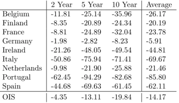
Table2summarises the cumulative effects for all events for some selected maturities. Accordingly, we see the strongest average (across maturities) reduction in yields from portfolio rebalancing for Portugal (85.80 BPS), followed by Italy (69.67 BPS) and Spain (62.11 BPS). In total, German yields have only been lowered by 5.91 BPS. Note, however, that one would expect stronger effects from portfolio rebalancing for longer maturities of 20 or 30 years which we, unfortunately, cannot measure. Also, we find rather small effects from the signalling channel measured as the change in OIS rates.
One explanation for the weak effects on Euro Area core countries’ bonds could be the institutional set up of the APP such as the ECBs regulation of not purchasing bonds below the deposit facility. Despite we do see the expected decreases for early announcements, cumulative spreads do often not react any more for later announcements, especially for German Bunds at several shorter maturities. This is due to
Table 2: Cumulative Impact of APP Press Releases on Selected Maturities in BPS
2 Year 5 Year 10 Year Average
Belgium -11.81 -25.14 -35.96 -26.17 Finland -8.35 -20.89 -24.34 -20.19 France -8.81 -24.89 -32.04 -23.78 Germany -1.98 -2.82 -8.23 -5.91 Ireland -21.26 -48.05 -49.54 -44.81 Italy -50.86 -75.94 -71.41 -69.67 Netherlands -9.98 -21.90 -25.88 -21.46 Portugal -62.45 -94.29 -82.68 -85.80 Spain -44.68 -69.63 -61.45 -62.11 OIS -4.35 -13.11 -19.84 -14.17
the imposed condition that the yield of a bond has to be above the deposit facility. Also the regulations with respect to the issue and issuer limit described in section2could undermine the market’s credibility in the ECBs ability of successfully implementing its QE programme. This might be one reason for the weaker response at later events.
An alternative explanation why we measure such mild effects for core countries is that the ECB mostly bought longer-term bonds which we would not observe in our data set. Unfortunately, the ECB does not publish much details about the bonds bought other than some aggregate information. However, the ECB claims that its interventions are intended to be market-neutral with respect to maturity31, i.e. there is no bias towards any specific maturities. Also, the weighted average maturity bought, which is published by the ECB, is comparably low for e.g. Germany and mostly stable in the observation period suggesting that this explanation is unlikely to hold32.
In our view, the most likely explanation for the weak effect on German Bunds is that the portfolio rebalancing channel might not have work to the same extend as for other countries. As theory suggest, portfolio rebalancing can only work if assets are not perfect substitutes, i.e. if investors have a preferred habitat motive, whereas, if assets are perfect substitutes quantitative easing is doomed to fail at the zero lower bound. Given the exceptional standing of German Bunds investors might consider them as being more closely to a perfect substitute of the risk free rate than other government bonds, for which we measure stronger effects. In contrast, countries with higher bond yields did show a more pronounced reduction suggesting that the portfolio rebalancing channel work more effective for these countries.
7
Regression Analysis
In order to provide a more detailed analysis, we run several event regressions in a similar spirit as in Szczerbowicz (2015) and Altavilla et al. (2015). Event regressions assume that markets are infor-mationally efficient meaning that new pieces of information immediately enter into prices of stocks or bonds. Therefore, assuming that price movements are essentially characterized by a random walk in
31
For more details see the ECB’s websitehttps://www.ecb.europa.eu/mopo/implement/omt/html/pspp-qa.en.html. 32
the absence of information using standard OLS techniques provides a reliable estimator to measure the significance of a single event day. Following this general approach, we proceed in two steps. In a first event regression, we measure how core and periphery bond yields were affected by each identified APP press release separately. In fact, most APP releases positively surprised the markets, leading to a drop in bond yields. Yet, some releases led to an increase in bond yields as markets where largely disappointed by the new piece of information. In a second regression, we group all identified events together into a single dummy variable to measure the average effect from QE on each country. In doing so, we also estimate the relative strength of the different asset price channels described earlier.
More precisely, in our first model we run separate regressions on the conditional change for each bond yield∆y(bond)m,it|y(bond)t
−1>DFt over a two day window of some selected maturities taking the set of our
ten event dummies as explanatory variables. Note that the superscript m distinguishes between core
and periphery countries. Also, we are including a wide range of control variables to measure the surprise effect of other macroeconomic news announcements for our respective period of interest. This yields the following estimator
∆y(bond)m,it|y(bond)t
−1>DFt= k X i=1 αiAPPi,t+ k X i=1
βiNewsi,t+γ∆y(bond)m,it−1+ǫt (5)
where APPi,t denotes all our identified APP announcement and speculation events individually,
Newsi,t represents a term for other news announcements, and ǫt is an error term. A detailed overview
about other news variables and how they are constructed is provided in the Appendix in table7. Not surprisingly, running several tests for heteroscedasticity and autocorrelation suggest that both are very likely in our data set. The F-Test for the event dummies and control variables coefficients is jointly tested and rejected under the zero-null hypothesis. To correct for both serial correlation and heteroscedasticity in the error terms, Newey-West standard errors for coefficients are used when estimating OLS. Also, ∆y(bond)m,it−1 denotes a lag to address first order auto-regression.
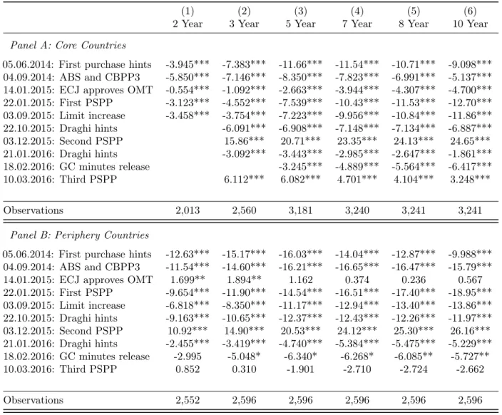
Table3shows the results of the basic event regressions for some selected maturities, controlling for the surprise component of a wide range of other macroeconomic news releases. As we are mostly interested in the relevance and general impact for each event day we only show the respective event dummies, suppressing the output of other control variables to examine potential heterogeneous effects among APP press releases33. Our results are mostly supportive for the conclusions drawn in the previous section. Most events show the anticipated sign of a reduction in yields both for core and periphery countries. The coefficients for periphery countries are usually larger compared to core countries which could be due to an implicit reduction in credit risk for periphery countries. Also consistent with previous findings, some press releases seem to have disappointed the markets leading to an increase in yields. In particular, the December announcement of 2015 has increased the yield for both core and periphery countries by several basis points. For core countries, the 3rd PSPP Announcement in March has also increased the
33
Note that due to serial correlation of the error terms the estimator are not efficient in this case. However, as serial correlation does generally not lead to a bias we do not consider this an issue here.
yield whereas it is negative but not significant for periphery countries.
Another finding we can confirm from the previous section is that for the majority of cases the change in the conditional yield is more pronounced for mid- and longer maturities. In contrast, short-term maturities are usually less affected, if not even excluded from purchases. For example, this is largely the case for the first announcement of the PSPP on the22nd of January 2015.
Table 3: Event Regression on the Conditional Change in Bond Yield
(1) (2) (3) (4) (5) (6)
VARIABLES 2 Year 3 Year 5 Year 7 Year 8 Year 10 Year
Panel A: Core Countries
05.06.2014: First purchase hints -3.945*** -7.383*** -11.66*** -11.54*** -10.71*** -9.098***
04.09.2014: ABS and CBPP3 -5.850*** -7.146*** -8.350*** -7.823*** -6.991*** -5.137***
14.01.2015: ECJ approves OMT -0.554*** -1.092*** -2.663*** -3.944*** -4.307*** -4.700***
22.01.2015: First PSPP -3.123*** -4.552*** -7.539*** -10.43*** -11.53*** -12.70*** 03.09.2015: Limit increase -3.458*** -3.754*** -7.223*** -9.956*** -10.84*** -11.86*** 22.10.2015: Draghi hints -6.091*** -6.908*** -7.148*** -7.134*** -6.887*** 03.12.2015: Second PSPP 15.86*** 20.71*** 23.35*** 24.13*** 24.65*** 21.01.2016: Draghi hints -3.092*** -3.443*** -2.985*** -2.647*** -1.861*** 18.02.2016: GC minutes release -3.245*** -4.889*** -5.564*** -6.417*** 10.03.2016: Third PSPP 6.112*** 6.082*** 4.701*** 4.104*** 3.248*** Observations 2,013 2,560 3,181 3,240 3,241 3,241
Panel B: Periphery Countries
05.06.2014: First purchase hints -12.63*** -15.17*** -16.03*** -14.04*** -12.87*** -9.988***
04.09.2014: ABS and CBPP3 -11.54*** -14.60*** -16.21*** -16.65*** -16.47*** -15.79***
14.01.2015: ECJ approves OMT 1.699** 1.894** 1.162 0.374 0.236 0.567
22.01.2015: First PSPP -9.654*** -11.90*** -14.54*** -16.51*** -17.40*** -18.95*** 03.09.2015: Limit increase -6.818*** -8.350*** -11.17*** -12.94*** -13.40*** -13.86*** 22.10.2015: Draghi hints -9.163*** -10.65*** -12.37*** -12.43*** -12.26*** -11.97*** 03.12.2015: Second PSPP 10.92*** 14.90*** 20.53*** 24.12*** 25.30*** 26.16*** 21.01.2016: Draghi hints -2.455*** -3.419*** -4.740*** -5.384*** -5.475*** -5.229*** 18.02.2016: GC minutes release -2.995 -5.048* -6.340* -6.268* -6.085** -5.727** 10.03.2016: Third PSPP 0.852 0.310 -1.901 -2.710 -2.724 -2.662 Observations 2,552 2,596 2,596 2,596 2,596 2,596
Notes: Conditional change of bond yield over a two day window as the dependent variable. The error terms are assumed to be heteroscedastic and possibly serial correlated up to a lag of 250 observations (i.e. daily data). Additional control variables are included but suppressed in output. Time frame is from 01.01.2014 - 30.06.2016. Number of observations varies as the spread is calculated as the conditional spread.∗ ∗ ∗=p <0.01,∗∗=p <0.05, and∗=p <0.1.
Finally note that there is no output produced for many two year core country bonds at later events due to our prior imposed condition that the yield of a given bond must be above the deposit facility. Currently, we have excluded these bonds as they cannot be bought by the ECB. However, one could also relax this condition34.
34
As a robustness check, we also estimated regressions without this constraint (available upon request). The results indicate that the yields on the excluded bonds actually often increase over the event window rather than decreases. One
In order to provide a more detailed analysis on a country specific level, we also estimate the average effect of our ten events by grouping them into one dummy. As illustrated in section 4, the yield of a country’s bond can be influenced by several channels through QE announcements. In the following, we proxy the strength of each of this channel for all countries directly by estimating the following equation taking the change in OIS rates (signalling channel), the change in bid-ask spreads (liquidity channel), the change in CDS premia (credit risk channel), and the change in the bond-OIS spread (portfolio
rebalancing) over a two day window as the dependent variable. For each country n, this yields the
following regression
∆ytn,i|y(bond)t
−1>DFt =αAll Eventst+
k
X
i=1
βiNewsi,t+γ∆ytn,i−1+ǫt, (6)
where ∆ytn,i|y(bond)t
−1>DFt denotes each of the four dependent variables (OIS rate, bid-ask spread,
CDS premia, and bond-OIS spread), respectively. To address serial correlation of the error terms again Newey-West standard errors are used.
As already discussed, taking the bond-OIS spread to measure the strength of the portfolio rebalancing channel is subject to two crucial assumptions, namely no liquidity and no credit risk for any given bond. In order to account for any unobserved changes in credit or liquidity risk, we include the contemporaneous changes in the country specific daily CDS premia and bid-ask spreads as additional control variables in our event regression. Moreover, to address concerns about potential macro spill-overs, which could reduce the perceived unobserved credit risk by investors’ general sentiment, we also include the Euro Stoxx 50 Volatility Index (VSTOXX) being sometimes referred to as the Fear Index. Including changes in both the VSTOXX index as well as a 10 year US treasury bond also gives the benefit of controlling for any other unobserved market news. In sum, our extended event regressions on the portfolio rebalancing channel for each countrynread as
∆Spn,it|y(bond)t −1>DFt =αAll Eventst+ k X i=1 βiNewsi,t+γ∆Sp n,i t−1+ k X i=1 θi∆Xi,t+ǫt (7)
where, ∆Spn,it|y(bond)t
−1>DFt is the conditional bond-OIS spread over a two day window and ∆Xi,t
denotes all other control variables each defined as the change over a two day window. Again details about the additional control variables can be found in table7.
reasons for this unexpected result could be that some investors speculated that the ECB could lower the deposit facility or even abolish the “no purchases below the deposit facility” rule. Thus, speculative investors would have bought such bonds shortly before an event and then, after the unchanged policy was released, sold these bonds again creating downward pressure on prices and increasing the yield.
Table 4: Measuring Average Effect of QE From Different Channels
(1) (2) (3) (4) (5)
VARIABLES OIS Bid-Ask CDS Portfolio Portfolio
Panel A: Belgium
All Events -1.050** -0.688*** -0.505*** -2.336*** -2.194***
Delta Bid-Ask 0.0155
Delta CDS Premia 0.0682***
Delta VSTOXX 0.0610***
Delta US 10y Bond -2.626***
Panel B: Finland
All Events -0.650 0.107* -0.202*** -1.703*** -1.575***
Delta Bid-Ask -0.00462
Delta CDS Premia 0.364***
Delta VSTOXX 0.0196
Delta US 10y Bond 0.302
Panel C: France
All Events -0.943 -0.249 -0.544*** -1.843*** -1.616***
Delta Bid-Ask -0.0185*
Delta CDS Premia 0.183***
Delta VSTOXX 0.0869***
Delta US 10y Bond 0.805
Panel D: Germany
All Events -0.798 1.272*** -0.469*** -0.499* -0.796***
Delta Bid-Ask 0.0597***
Delta CDS Premia -0.0405***
Delta VSTOXX -0.116***
Delta US 10y Bond 1.493***
Panel E: Ireland
All Events -1.012* 3.836*** -0.555*** -2.219*** -1.309***
Delta Bid-Ask 0.0182**
Delta CDS Premia 0.838***
Delta VSTOXX 0.254***
Delta US 10y Bond -5.290***
Panel F: Italy
All Events -0.691 1.130*** -4.736*** -5.183*** -0.526
Delta Bid-Ask -0.0356***
Delta CDS Premia 0.620***
Delta VSTOXX 0.305***
Delta US 10y Bond -4.050***
Notes: Change in OIS rate (signalling channel), bid-ask spread (liquidity channel), CDS premia (credit risk channel), and conditional change in bond-OIS rate (po