A COUNTERFACTUAL ANALYSIS OF REGULATORY
CHANGES IN HUNGARY: COULD THE FX LENDING
CRISIS HAVE BEEN AVOIDED?*
Dóra SIKLÓS(Received: 22 June 2015; revision received: 19 October 2015; accepted: 8 December 2015)
DÓRA SIKLÓS
The main purpose of this paper is twofold. First, it aims to estimate the effect of the tightening of regulatory capital requirements on the real economy in periods of credit upswing. Second, it intends to show whether applying a counter-cyclical capital buffer measure as set down in the Basel III rules could have helped to reduce the pace of FX lending growth in Hungary, mitigating the build-up of vulnerabilities in the run-build-up to the global fi nancial crisis. In order to answer these questions, we use a Vector Autoregression-based approach with the aim of understanding the impact of shocks to capital adequacy in the pre-crisis period. Our results suggest that although regulatory authori-ties could have slowed down the increase in lending temporarily, they would not have been able to avoid the upswing of FX lending by requiring counter-cyclical capital buffers even if such a tool had been available and even if they had reacted quickly to accelerating credit growth. Our results also suggest that a more pronounced tightening might have reduced FX lending substantially, but at the expense of real GDP growth. The reason is that unsustainable fi scal policy led to a trade-off between economic growth and the build-up of new vulnerabilities in the form of FX lending.
JEL classifi cation indices: E58, G01, G21, G28
Keywords: FX lending, capital adequacy, bank regulation, counterfactual analysis
* I am grateful for Balázs Csontó for his suggestions and encouragement that provided the impetus for this project. The views expressed in this paper are those of the author and do not necessarily reflect the views of the European Stability Mechanism.
Dóra Siklós, Banking sector expert, member of the staff of the European Stability Mechanism (ESM). E-mail: d.siklos@esm.europa.eu
1. INTRODUCTION
The global financial crisis (GFC) shed light on the importance of the so-called macro-financial linkages through which the activity of the financial sector could have a tangible impact on economic activity. At the same time, it was also made clear that neither pre-crisis financial supervisory practices, nor monetary policy succeeded in ensuring financial stability. As part of a general reassessment of economic policies, macroprudential policies gained traction and have become a part of the overall policy response to the challenges posed by the crisis.
The adoption of these policies has been complicated by several factors (Clas-sens 2014). First, macroprudential policies should be motivated by externalities and market failures. However, there is no clear guidance on the design of these policies. Second, given that most countries decided to resort to macroprudential policies only recently, there is limited experience and empirical analysis on their efficiency.
Similarly to other countries, Hungary also had to realise the importance of macro-financial linkages. However, in contrast to several other countries that ex-perienced an asset price boom and/or excessive credit growth in the pre-crisis period, the main source of the Hungarian vulnerability was the currency mis-match stemming from the foreign currency – mostly Swiss franc – borrowing by households and corporations as well as the maturity mismatch of banks. Spe-cifically, the banking sector financed its long-term foreign currency lending with short-term off-balance sheet transactions (mostly FX, but also currency interest rate swaps). The impact on the banking sector of the GFC was at least threefold. First, increased risk aversion in global financial markets resulted in a flight to safe assets, including the Swiss franc. The rising debt service of households and corporations stemming from the appreciation of the Swiss franc then led to an increase in the losses of banks on their loan portfolio. Second, banks had to meet margin calls on their FX swaps due to the depreciation of the Hungarian forint. Third, all banks had difficulties in rolling over their short-term FX swaps during initial period of the crisis.
In this paper, we apply a counterfactual analysis with the aim of assessing whether excessive credit growth and the build-up of FX loans could have been prevented by the use of macroprudential policies. Specifically, by estimating the historical relationship between aggregate capital adequacy, lending, and a set of macroeconomic variables, we calculate an alternative scenario of pre-crisis lend-ing based on a hypothetical capital adequacy regulation.1
1 Based on IMF (2000), aggregate capital adequacy ratio is considered to be a macroprudential
The structure of the paper is as follows. Section 2 reviews the literature. Sec-tion 3 gives an overview on the motivaSec-tion of the analysis. SecSec-tions 4 and 5 de-scribe the data and the estimation technique, respectively. Section 6 summarises the estimation results, while Section 7 concludes.
2. RELATED LITERATURE
Given the brief history of the application of macroprudential policies, there are only a small number of empirical papers analysing the efficiency of these tools. Estimating the effect of macroprudential rules is complicated for at least two reasons: (i) they rarely existed before the GFC, and (ii) those already in place (es-pecially the capital adequacy ratio) were broadly stable in the pre-crisis period.
Based on the applied method, we can group the existing international literature into two categories:
1. Bottom-up approach, i.e. estimations using micro-level data
Bridges et al. (2014) analysed the effect of changes in the regulatory capital requirements on lending, based on bank-level data. They used estimation results from panel regressions of lending to different sectors on regulatory capital requirements and observed capital ratios to build impulse responses with the aim of understanding the effects of a perma-nent 1 percentage point increase in capital requirements. Although the results vary across sectors, they found that an increase in capital require-ments reduces loan growth with a lag of one year and a recovery within three years. The cumulative effect of a 1 percentage point increase in the regulatory capital on loan volumes is –3.5% after 12 quarters. Brun et al. (2015) used loan-level data in France with the aim of estimating the effect of an easing of the capital requirement on corporate lending. Their time span covered the transition from Basel I to Basel II in or-der to estimate the elasticity of corporate lending to capital requirement. They found a relatively large effect of capital requirements on lending, i.e. a 1 percentage point decrease in capital requirements led to a 0.75% growth in outstanding corporate loans. Berrospide et al. (2010) examined the effect of capital injection programmes in the US, such as that of the Capital Purchase Program (CPP). They carried out both panel regression and VAR-based analysis, and found only a modest effect of capital on lending. According to their results, a 1 percentage point increase in the capital-to-assets ratio triggered an increase of 0.7–1.2 percentage point in lending growth.
2. Top-down approach, i.e. estimations using aggregated data
As a part of their impact studies for Basel III,BIS (2010) implemented two different one-step top-down approaches for estimating the effect of increasing capital requirements. First, they used DSGE models that ex-plicitly incorporated the banking sector. The results are modest, with a 1 percentage point increase in the target capital adequacy ratio leading to a decrease of 0.14% in output after 18 quarters. Second, they estimated VAR models that included standard macroeconomic variables such as real GDP growth, GDP deflator and interest rates as well as banking sec-tor variables such as aggregate bank loans and capital/assets ratios. The results from these estimations were more pronounced, with a 1 percent-age point increase in the target capital ratio leading to a 0.4% decrease in output. Noss – Toffano (2014) assessed the impact of changes in capital requirements on lending in the United Kingdom, by estimating a SVAR model. They assumed that an increase in banks’ capital requirements have a negative effect on lending at least in the short run. This assump-tion is necessary to understand to what extent the change in bank lending behaviour was a result of the increasing capital requirement, rather than broader macroeconomic developments. They found that a 15 basis point increase in capital requirements during an economic upswing is associ-ated with a 1.4 percentage point decrease in lending after 16 quarters. At the same time, its effect on GDP was found to be insignificant.
A few studies aimed to estimate specifically the effect of changes in regula-tory capital in Hungary. Following the introduction of regulations based on Ba-sel II, Zsámboki (2007) investigated their potential consequences, in particular on financial stability. He pointed out that given the pro-cyclical nature of the regulation, banks should build up capital reserves above the regulatory minimum requirements during an economic upswing in order to be able to cover any future losses. Although the analysis drew attention to the pro-cyclical nature of the Basel II regulation, it did not examine its potential effect on the real economy. Szombati (2010) analysed the macroeconomic effect of Basel III rules. She found that a 1 percent (equivalent to around 13 basis points) increase in the capital require-ment is associated with a decrease of 0.63–1.05% in real GDP after 32 quarters. These results were based on the assumptions that (i) the banking sector adapts to the new regulation by capital increases and reduction in assets in an equal meas-ure, (ii) the adjustment would be faster in corporate lending than in the household lending, and (iii) banks with a larger capital buffer could take over loans from other banks with lower capital buffers.
Tamási – Világi (2011) and Hosszú et al. (2013) estimated a Bayesian VAR model for the Hungarian economy and applied sign restrictions to identify macr-oeconomic and credit supply shocks. Assuming that different types of credit sup-ply shocks might require different policy responses, they analysed the effect of changing risk assessment of financial institutions as well as that of changing reg-ulatory requirements (credit spread shock). They found that the impact of the two shocks differs substantially. In the case of changing risk assessment, the response of credit portfolio and real GDP are much more pronounced and permanent than in the case of a credit spread shock. Their results show that changing risk assess-ment indicates a 1% decrease in lending and a 0.21% decrease in real GDP, while changing regulatory requirements has a negative effect of 0.18% on real GDP. The order of magnitude and the permanence of the response of real variables could be explained by the fact that the underlying VAR model contained only corporate loans whose duration is typically lower than that of households.
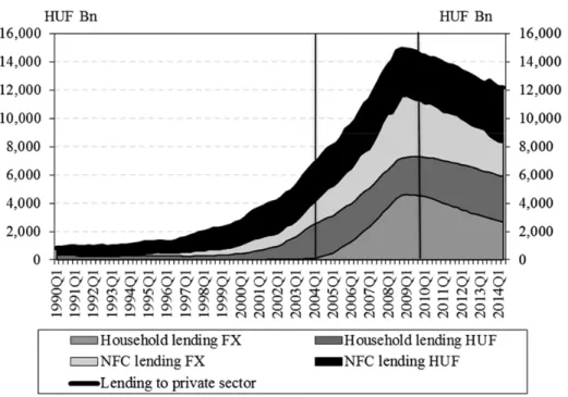
3. MOTIVATION: EXCESSIVE BORROWING IN FOREIGN CURRENCY? Private sector borrowing in Hungary increased substantially between 2004 and 2009, mostly driven by foreign currency (Swiss franc) denominated loans. Both non-financial corporations and households increased their foreign currency bor-rowing, but it was more pronounced in the household sector.
Using four different trend-filtering methods, Hosszú et al. (2015) showed that the initially negative credit gap turned into a significant positive credit gap both in the household and corporate sectors. Their results are mostly in line with that of Holló (2012) who found that the imbalances in the Hungarian banking system, namely the excessive credit growth and the sharp increase in the ratio of total li-abilities to stable funds, started to emerge in the last quarter of 2005 and lasted until the onset of the financial crisis. Kiss et al. (2006) concluded that although credit growth between 2004 and 2005 was somewhat faster than its equilibrium rate,2 this can be justified by convergence. It implies that it was not the speed of
lending growth per se that should have given rise to concerns, but rather its cur-rency composition, i.e. the excessive lending in foreign curcur-rency.
There are several possible explanations for why foreign currency lending gained momentum in Hungary. In order to find explanations, we first try to iden-tify whether the motivation originated from the demand or the supply side.
2 Equilibrium level is identified by some fundamental macroeceonomic variables for developed
Bethlendi et al. (2005) found that the increase in FX lending, which started in 2004, was mostly due to rising demand, possibly reflected by the opening of Hun-garian banks’ on-balance sheet FX position and their increasing loan-to-deposit ratio.
Bethlendi et al. (2005), Rosenberg – Tirpák (2008),andCsajbók et al. (2010) identified the following factors on the demand side that presumably contributed to the increase in FX lending. The first three are more relevant for households, while the fifth concerns mostly non-financial corporations.
– Interest rate differentials: The increasing share of FX lending in the private
sector stems from a portfolio allocation decision based on the uncovered inter-est rate parity. Specifically, the dominter-estic interinter-est rate is equal to the sum of the foreign interest rate, the expected depreciation of the exchange rate, and the exchange rate risk premium. As long as the risk awareness of borrowers is the same as the sum of expected exchange rate movements and exchange rate risk premium, changes in interest rate differential do not induce substitution between domestic and foreign currency loans. Substitution only happens if exchange rate expectations are not homogeneous. Since households had rela-tively good experiences with consumer FX loans, their risk sensitivity against
exchange rate and interest rate was probably quite low. This led households to borrow in foreign currency, given the substantial interest rate differential. The latter was also an important factor for non-financial corporations operating in the non-tradable sector (Bodnár 2006), and therefore they became exposed to exchange rate risks to a similar extent as households did.
– ‘Fear-of-floating’ factor: In the lack of fixed-rate domestic currency loans,
borrowers might weight the risks associated with floating-rate domestic cur-rency loans against foreign curcur-rency loans. Specifically, to the extent domes-tic currency interest rate volatility exceeds exchange rate volatility, borrowers might find foreign currency borrowing more attractive. This can be reinforced by the monetary authority, if it uses interest rate policy to smooth exchange rate movements.
– Liquidity constraint: If a household is not able to pay more than a certain
pro-portion of its income to service its debt, the size of the monthly debt serv-ice and its variance are crucial factors. Most households could not afford the higher monthly repayment of HUF loans. Typically, households with stronger liquidity constraints generated the demand for cheaper FX loans. Moreover, the longer the maturity of the loan, the larger the effect of the interest rate dif-ferential on the monthly repayments.
– Regulatory changes: The tightening of the eligibility criteria of subsidised
mortgage loans in 2004 could also have prompted households to switch to cheaper FX loans.
– Hedging FX deposits: It is mostly related to non-financial corporations that
have FX revenues. In order to hedge their FX income, these entities borrowed in foreign currency.
On the supply side, the authors mention that the availability of foreign funds stemming from strong financial ties between domestic commercial banks and their parent banks residing in the EU might also have influenced the currency composition of loans.
The private sector’s increasing demand for FX loans increased the banking sector’s need for FX funds. Hungarian banks collecting mostly HUF deposits had two options to fulfil this need: on-balance sheet foreign currency financing, typi-cally from parent banks and/or off-balance sheet swap transactions. Both forms of FX funding contributed to the build-up of macroeconomic vulnerability. First, risks related to on-balance sheet FX funding stem from the increasing external debt of the country. Moreover, banks typically financed long-term mortgage FX loans with short-term foreign funds, leading to a maturity mismatch and thus substantial roll-over risks as well as potential reliance on emergency FX liquidity facilities.
Second, synthetically creating FX exposure through swaps is even riskier. In addition to the fact that it increases the country’s external debt,3 it has further
drawbacks: (i) while foreign funds enhance liquidity, increasing the balance sheet of the banking sector, FX swaps only change the denomination of existing liquid-ity without any change in total liquidliquid-ity and balance sheet; (ii) the maturliquid-ity of FX swaps has been generally shorter than that of foreign funds. As a result, the rollover risk is even higher than in the case of foreign funds.
These vulnerabilities had serious consequences for Hungary during the crisis when risk aversion intensified and investors flew to safe-haven currencies, such as the Swiss franc. First, the weakening of the Hungarian forint against the Swiss franc substantially increased the monthly repayments for households. Eventually, this resulted in increasing non-performing loan (NPL) ratios as well as decreasing consumption and investments. Second, the renewal of foreign funds and swaps be-came more expensive as the country’s and the parent banks’ CDS spreads, the most important pricing component, increased substantially (Páles – Homolya 2011). 3 Assuming that the foreign counterparts place their HUF liquidity in the Hungarian banking
sector.
The prevalence of FX loans played an important role in the deepening of the crisis. Increasing funding costs and NPL ratios put pressure on the banking sec-tor’s income-generating capabilities, limiting its ability to contribute to real GDP growth. As such, it is of great importance to examine whether the excessive FX lending could have been avoided by requiring a counter-cyclical capital buffer as set down in the Basel III rules and if so, at what macroeconomic costs.
In this paper, using a Vector Autoregression Model (VAR), we estimate the effect of changes in regulatory capital requirements based on the pre-crisis rela-tionship between the aggregate capital adequacy ratio and other macroeconomic variables. The results could provide policymakers with a sense on the macroeco-nomic effect of changes in macroprudential capital requirements.
4. DATA
In the previous section, we identified 2004–2009 as a period of credit upswing in Hungary. The start of this period was chosen to be 2004 since there was broadly no FX lending to households before 2004. Lending to the private sector increased on a year-to-year basis even after the onset of the GFC until the end of 2009, therefore we consider it as the turning point. In the estimation, the following quarterly variables were used for this period:
– Real GDP growth: The source of the data is the Hungarian Central
Statisti-cal Office. Seasonally adjusted growth rates were used for the estimation.
– Growth rate of real lending to private sector: Data published by the central
bank of Hungary (MNB). We adjusted growth rates seasonally and for ex-change rate ex-changes.
– Alternative funding sources (growth rate): It refers to non-financial
corpora-tions (NFCs) and includes loans from non-financial entities, other financial corporates, public institutions, households, and foreign entities as well as bonds issued by non-financial corporates. Data are seasonally and exchange rate adjusted and published by MNB. Since bank financing is by far the most dominant form of funding for corporates in Hungary, the explanatory power of this variable might be limited. However, given its importance in some segments of the economy, we decided to include it in the baseline model. More importantly, the inclusion of alternative funding is necessary in order to be able to simulate a credit supply shock.
– Hungarian sovereign CDS spread represents the FX funding costs of the
Hungarian banking sector. Páles et al. (2011) showed that before the onset of the crisis, Hungarian banks were able to obtain foreign funds at levels corresponding to those of their parent banks and Hungarian sovereign CDS
spreads. Between the onset of the crisis and 2009, both the funding costs of parent banks and Hungarian sovereign CDS spreads increased substantially. Although the funding costs of Hungarian banks remained at the level of those of their parent companies during this period, they started to decouple significantly at the beginning of 2010. As a result, the Hungarian sovereign CDS spread seems a good proxy for the funding costs of banks between 2004 and 2009. CDS spreads were downloaded from Bloomberg.
– Hungarian 3-month money market rate (BUBOR): Similarly to CDS
spreads, this variable is used to capture Hungarian banks’ HUF funding costs. BUBOR is expected to have an impact through the substitution chan-nel, i.e. the higher the HUF borrowing costs, the more households move towards borrowing in FX. The MNB publishes data on a monthly basis.
– Real Effective Exchange Rate (CPI based REER): The variable measures
the country’s competitiveness compared to its main international trade part-ners. Time series are published by the MNB.
– Capital Adequacy Ratio (CAD ratio): Data are coming from regulatory
reports submitted to the MNB. The denominator of the ratio is the risk-weighted assets of the banks and is calculated according to the Basel II rules.4 Although there are arguments for using total assets instead of
risk-weighted assets in order to filter out the effect of any potential attempts made by banks trying to alter their balance sheet, the official CAD ratio still seems a better alternative, given that the main purpose is to quantify the ef-fect of changes in the CAD ratio. The capital adequacy ratio required under Pillar II by the authorities differs from bank to bank, but we assume that there is no bank with a higher required capital adequacy ratio than the sec-tor average. This assumption ensures that an increase in the required capital ratio would lead to a decrease in banks’ capital buffer.
The first three variables are expressed as growth rates, in the case of BUBOR and REER, their levels are used, while CDS spreads and the aggregate capital adequacy ratio are in first difference in order to ensure their stationarity. As a pre-liminary attempt, the levels of these variables were used, but the estimated VAR did not satisfy the stability criteria.
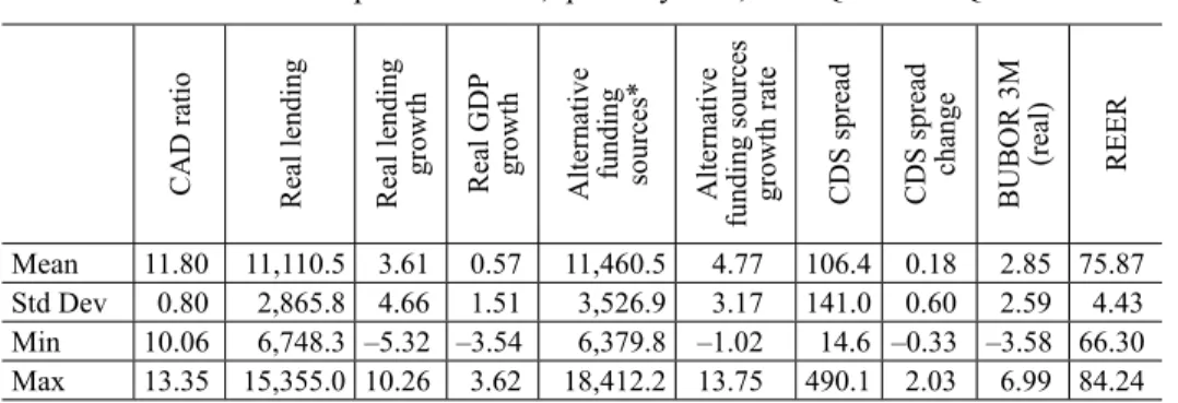
Table 1 shows the descriptive statistics of the variables. In addition, it is worth
noting that real GDP is positively correlated with real lending, alternative fund-ing, and the aggregate CAD ratio (albeit only weakly in the latter case), while it is 4 Although the impact of an increase of the CAD ratio is likely to depend on the composition
of capital injection (e.g., common equity versus subordinated debt), the limited availability of data does not allow for distinguishing between different types of capital injection.
negatively correlated with the Hungarian sovereign CDS spreads. Real lending is negatively correlated with alternative funding, CDS spreads, BUBOR, and CAD ratio. Notwithstanding the intuitive relations between the variables, the contem-poraneous correlations do not differ significantly from zero in most cases, sug-gesting that lagged values might have better explanatory power.
Thecorrelation of lagged lending and contemporaneous GDP, i.e. the correla-tion between lending growth in period t + lag and GDP growth in period t, as well as between lagged CAD ratio and lending growth show that lending growth in any period has the highest correlation with GDP growth two quarters earlier. This suggests that corporations and households tend to arrange credit facilities during economic upswings, so that they have liquidity buffers during periods of down-turn. The relationship between the lagged CAD ratio and lending growth seems to confirm the pro-cyclical behaviour of the banking sector: banks increase their leverage during upturns by increasing lending.
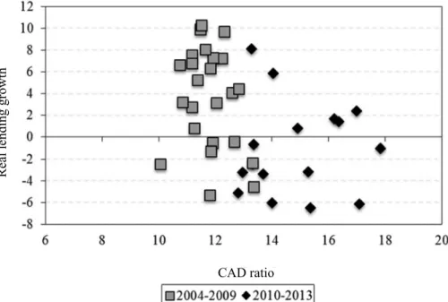
The expected relationship between banks’ capital adequacy ratio and real lend-ing is also supported by post-crisis data. Between 2004 and 2009, capital ratios decreased as lending expanded, while it has been the other way round in recent years.
5. MODEL
Our first goal is to understand the impact of changes in capital requirements on banks’ funding costs. Based on the Modigliani–Miller (M&M) theorem (1958), an increase in the regulatory capital requirement does not change banksʼ overall funding cost. However, this statement is conditional on a number of underlying
Table 1. Descriptive statistics, quarterly data, 2004Q1 – 2009Q4
CAD ratio Real lending Real lending growth Real GDP growth Alternative funding sources* Alternative
funding sources growth rate CDS spread CDS spread
change BUBOR 3M (real) REER Mean 11.80 11,110.5 3.61 0.57 11,460.5 4.77 106.4 0.18 2.85 75.87 Std Dev 0.80 2,865.8 4.66 1.51 3,526.9 3.17 141.0 0.60 2.59 4.43 Min 10.06 6,748.3 –5.32 –3.54 6,379.8 –1.02 14.6 –0.33 –3.58 66.30 Max 13.35 15,355.0 10.26 3.62 18,412.2 13.75 490.1 2.03 6.99 84.24
Note: * It contains bond issuance, other non-FI loans, and loans from abroad of NFC.
assumptions, including the absence of frictions and taxes. In reality, the M&M theory does not hold for the following reasons:
– Taxes: Since interest payments on debt are tax-deductible, banks have an
incentive to operate with higher leverage.
Admati – Hellwig (2013) highlight two additional factors that create incen-tives for banks to increase leverage:
– Explicit state guarantee: Deposit insurance schemes reimburse losses not
covered by banks’ assets, thereby lowering banks’ funding costs. Moreover, during the recent financial crisis, governments extended guarantees even for non-deposit liabilities of banks.
– Implicit state guarantee: By reducing the funding costs of too-big-to-fail
institutions, it provides these banks with an advantage over other banks. As a result of these factors, banks’ funding costs are lower than they would otherwise be.
During the pre-crisis period, investors’ risk perception related to the financial sector was very small. As a result, banks were able to borrow at low rates. In this environment, an increase in capital requirements was considered to be a credit supply shock, i.e. it would have caused banks’ funding costs to increase. Possible
Figure 3. Real quarterly lending growth versus aggregate capital adequacy ratio CAD ratio
responses could have included the following: (i) decrease lending, (ii) increase retained earnings, or (iii) raise capital. However, the first option seems the most likely outcome, given some constraints associated with the second and third re-sponses. Specifically, an increase in retained earnings is constrained by sticky dividend payments and banks’ reluctance to reduce spending during economic upswing. Similarly, banks tend not to raise capital during these periods when they usually accumulated liquidity buffers. The reason is that investors are aware of the fact that a bank does not need to issue new equity, but if it does so, it would be a sign of the firm being overvalued (Myers – Majluf 1984).
The above relationship between banks’ funding costs and the level of the regu-latory capital ratio, however, might have changed after the crisis. Specifically, it changed from positive to negative, i.e. higher capital requirements are associated with lower funding costs. The GFC revealed significant imbalances in the finan-cial sector that were overlooked by investors in the pre-crisis period. In such an environment, an increase in the regulatory capital level could increase investors’ confidence in the banking sector, by supporting banksʼ resilience as well as their ability to increase lending (Noss – Toffano 2014).
Due to the above-mentioned ambiguous effect of an increase in the regulatory capital on lending, following Noss – Toffano (2014) we estimated two different models: (i) an unconstrained VAR model in which there are no assumptions re-garding the impact of a capital adequacy shock, and (ii) a Structural VAR (SVAR) where we introduced a sign restriction on lending and on alternative funding growth, i.e. an increase in capital requirements is associated with a reduction in lending and an increase in alternative funding. The latter reflects the assumption that the relationship between capital requirements and lending was negative be-fore the crisis. This way, the results stemming from the two models could serve as a reasonable range for policymakers to estimate the effect of macroprudential regulation on the real economy regardless of the economic cycle.
Notwithstanding the strengths of the approach, i.e. identifying capital adequa-cy tightening-like situations in the past to gauge the impact of future changes when such policy action is not present in the historical data, it has several caveats. For example, the change in the regulatory minimum does not necessarily require banks to increase their capital adequacy ratios since they typically hold buffers above the regulatory minimum level. As a result, the shock that we apply in the model could be interpreted in the following ways:
– Assuming banks intend to keep their buffers constant in longer terms, an in-crease in the regulatory capital requirement has a one-to-one effect on the capital adequacy ratios. Bridges et al. (2014) showed that regulatory capital requirements impact bank capital ratios, i.e. banks typically rebuild their buffers following a tightening of capital regulations.
– The change can reflect an increase in the applicable risk weights for FX loans that leads to an increase in the capital requirement and a decrease in capital buffers.
– The tightening can also be considered as an implementation of a counter-cyclical capital buffer as it is set down in the Basel III rules.
The primitive form of the Vector Auto Regression (VAR) model can be defined as follows (Enders 2010): 0 1 Γ Γ ε
p t i t i t i Bx x (1) wherep is the number of lags
xt is a vector of the endogenous variables
t realgdpt reallendingt cds spreadt alternative funding sourcest
CAD ratiot x
B contains the contemporaneous effect of a unit change of an endogenous vari-able on another endogenous varivari-able.
1 1 1 p p pp b B b b Γ0 is the constant 10 20 0 30 40 50 Γ b b b b b
Γ1 is a p x p matrix that contains the coefficients of the lagged endogenous variables 11 1 1 1 γ λ Γ γ γ p p pp
εt is the error term t t t t t realgdp reallending CDS spread t
alternative funding sources CAD ratio x ε ε ε ε ε
Multiplying equation (1) by B–1 allows us to obtain another VAR model in standard form, VAR(2):
0 1 p t i t i t i x A A x e
(2) where A0 = B–1Γ 0, A1 = B–1Γ1, and et = B–1εt .In this paper, two lags were used in the estimation of the VAR. According to the standard information criteria, three lags were supposed to be included in the model, but the resulting VAR did not satisfy the stability criteria. Moreover, the selection of two lags reflects the low degrees of freedom arising from having relatively few observations, relative to the number of variables in the model.
Sign restrictions were introduced, based on Fry – Pagan (2007).
The relationship between residuals from the standard form and those from the primitive form of the VAR is as follows: et = B–1ε
t. If there is an S matrix with
the estimated standard deviations of the εt on the diagonal and zeros elsewhere, we could express residuals as et = B–1SS–1ε
t = Tηt, where ηt = S–1εt has unit
vari-ances.
Assuming that there is a Q matrix such that Q'Q = QQ' = I, we can rewrite residuals as follows:
et = TQ'Qηt = T*η*
t.
This results in a new set of estimated shocks η*
t with a covariance matrix I
since E(η*
t;η*t) = QE(ηt;η't)Q' = I. As a result, we have a combination of the
shocks η*
t that have the same covariance matrix as ηt, but a different impact on et, hence the xt.
In order to create the above impulse responses and Q matrices, we take the following steps:
1. We compute E(et;e't) = Σ and assume that B–1, such that e
t = B–1εt;
3. We apply QR decomposition on K matrix so that K = QR, where Q is or-thogonal;
4. Q is orthogonal (QQ’ = I), therefore Σ = B–1QQB–1', that forms another pos-sible decomposition of the covariance matrix and B–1' = B–1Q;
5. We then repeat these steps 1,000 times and keep the results that satisfy the sign restrictions.
Interpreting the impulse responses that satisfy the scheme of imposed restric-tions is not straightforward, since the model that produced the median response for one variable might not be the same for the other variables. Fry – Pagan (2007, 2011) suggest a solution to this problem that chooses those impulses that are the closest to the median responses (Median Target Method). In order to implement it, we first need to standardise our results by subtracting the median from each impulse response value and divide it by its standard deviation over all models that satisfy the sign restrictions. These standardised impulses are placed in a vector
ϕ(1) for each impulse response value Θ(1). Subsequently we choose the l that mini-mises MT = ϕ(1)'ϕ(1) and then use Θ(1) to calculate impulse responses. This proc-ess does not necproc-essarily provide a unique l, but in our case, the closest impulse response to the median came from the same model for all variables.
6. ESTIMATION RESULTS
The VAR(2) model described in the previous section was estimated for a seven-equation system. The coefficients were jointly significant in each seven-equation.
The magnitude of the shock was chosen such that policymakers would have intervened to maintain capital adequacy ratios at their 2005Q1 level (12.04%t;
Figure4). This choice seems plausible as (i) it is greater than levels observed in
the pre-crisis period, but lower than levels seen in the aftermath of the crisis, and (ii) it is reasonable to assume that if a counter-cyclical capital buffer measure had been available, the authorities would have had enough time (four quarters after the start of the credit upswing) to react to increasing lending by requiring additional capital.
In the remainder of this section, we describe the impact of changes in capital requirements based on the results of both the unconstrained and the constrained models.
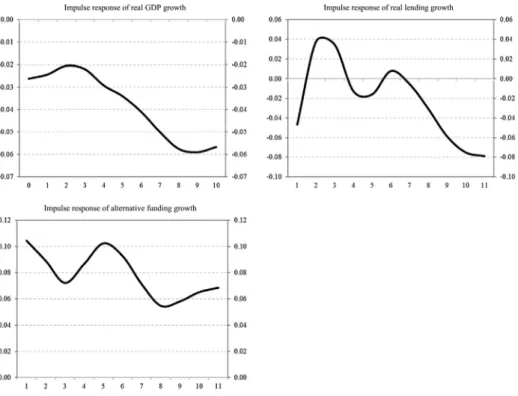
Figure 5 shows the unconstrained effects of a macroprudential tightening on
real GDP growth, real lending, and alternative funding growth. As we mentioned above, the unconstrained model intends to simulate the post-crisis behaviour of the banking sector and investors, i.e. a tightening of capital requirements does not
Figure 4. Aggregate CAD ratio
Figure 5. Impulse responses of a 13 basis point shock to the change in the aggregate CAD ratio
necessarily induce a credit supply shock. The response of real GDP growth to an increase in capital adequacy ratio is moderate; following a temporary increase, it returns to its pre-shock level after 10 quarters. The overall effect on real lend-ing growth is similar to that on real GDP, i.e. it returns to its initial level after 10 quarters, albeit the initial increase proves to be more persistent.
The reason for the increase in real GDP and lending as a response to increasing capital requirements is at least twofold. First, as we argued in Section 3, demand-side factors seemed to be the main drivers of lending growth, in particular FX lending growth. Our estimation results seem to confirm this. Specifically, the positive impact of higher capital adequacy on lending suggests that strong de-mand could actually have resulted in an even higher growth rate of lending. In other words, the latter was prevented by credit supply. As a result, an increase in capital adequacy could have let banks satisfy demand for loans to a higher extent and thus could have led to higher lending growth. Second, as indicated in Section 5, the relationship between capital adequacy and lending is ambiguous. Specifi-cally, if higher capital adequacy improves investor confidence in the banking sec-tor, it leads to lower funding costs, i.e. it could make it easier for banks to finance a further expansion in their loan portfolio.
Noss – Toffano (2014) found similarly weak positive responses for lending when they excluded the sign restriction. They explained it as lending being the only potential transmission channel for macroprudential capital requirements. It seems plausible in periods of credit upswing, when banks’ cost of debt is insensi-tive to their capital level.
The reaction of alternative funding growth to an increase in the capital re-quirement seems puzzling at first glance, as an increase in the supply of bank lending is associated with an increase in alternative funding, i.e. companies do not substitute bank funding with alternative sources. However, taking a closer look at the historical relationship of real lending growth and alternative funding growth could provide some explanation for this. As it is shown in Figure 6, lend-ing to corporations and fundlend-ing from alternative sources moved together until the onset of the GFC. This could be explained by two factors: either (i) corporations faced a scarcity of bank funding, i.e. bank and alternative funding complemented each other, or (ii) they used other funding channels for specific reasons (e.g., the signalling effect of bond issuance in the case of listed companies). Given that the model was estimated for the pre-crisis period, it captures this positive relation-ship between bank and alternative funding. As a result, a change in capital ad-equacy affects these funding sources in the same directions. However, the GFC revealed that this relationship might change during periods of distress. As the figure shows, bank funding decreased during the crisis, while alternative
fund-ing increased slightly, suggestfund-ing that companies that have access to alternative sources of funding substituted bank lending to some extent.
Figure 7 shows the results from the SVAR model, i.e. where sign restrictions
were introduced in order to simulate a credit supply shock. Specifically, an in-crease in the regulatory capital requirement is expected to lead to a dein-crease in lending and an increase in the alternative funding growth. In line with our prior expectations, such a policy change has a stronger impact on real variables than the unconstrained VAR; however, its overall effect remains modest.
Real GDP growth has a relatively modest immediate response; however, it strengthens after 10 quarters. This pace of reaction could be due to a number of factors. An increase in capital requirements immediately affects banks’ risk-tak-ing ability and thus reduces the availability of bank lendrisk-tak-ing for companies. The resulting cancelation or postponement of leveraged investment projects might have a more pronounced impact on GDP, as investments are partly financed with own resources. Moreover, the cancelation of investment has a multiplier effect on GDP. According to our results, lending growth also falls sharply in the third quarter, and after a temporary recovery, it continues to decrease afterwards. Al-ternative funding shows an opposite moving pattern, suggesting that companies seek for other funding sources as access to bank lending decreases. However, the
Figure 6. Lending to corporations and alternative funding sources
demand for alternative funding fades out after 10 quarters, as real GDP growth declines.
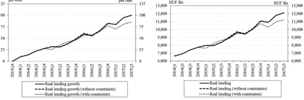
Using our estimation results, we conducted a counterfactual exercise. Specifi-cally, we calculated the hypothetical evolution of real GDP and lending in the presence of a shock to capital adequacy at the beginning of 2005. The alternative paths of real lending can be seen in Figure 8. An increase in capital requirements would have had a modest effect on lending: the difference between actual and counterfactual outstanding loans would have been in the range of around HUF –900 billion (constrained model) and HUF 5 billion (unconstrained model) at the end of the period. While actual lending to the private sector doubled in real terms during this period, it would have increased by 86% in the constrained counterfac-tual scenario, i.e. increasing capital requirements would have had only a moder-ate impact on lending.
Given that real lending would not have changed notably, tightening the regu-latory capital requirements would also have had a minor impact on real GDP
Figure 7. Impulse responses of a 13 basis point structural shock to the change in the aggregate CAD ratio
growth. Specifically, the difference between the actual and counterfactual cumu-lative real GDP growth is in the range of +0.2 to –6.5 percentage points after 10 quarters (Figure 9).
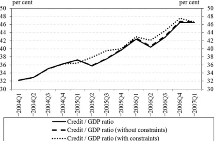
The overall effect of an increased regulatory capital level could not have slowed down the increase of the credit-to-GDP ratio. Although it could have held back the lending growth, but it would have inferred an equal drop in the real GDP growth. As a result, the difference in the ratio would have been only +0.1 percent-age points after 10 quarters.
The total impact of our hypothetical regulatory tightening would have been modest in terms of preventing the build-up of vulnerabilities in the banking sec-tor. Even in the case of a quick reaction of the regulatory authorities, the use of counter-cyclical capital buffer would not have been able to significantly lower either the level of lending or its growth rate.
Figure 8. Growth and level of real lending in the alternative scenarios
Figure 9. Growth and level of real GDP in the alternative scenarios
Although the overall impact of an increasing regulatory capital requirement is found to be modest, it is also interesting to see how this measure would have affected lending to different sectors. Since sectoral lending was not included in the VAR models due to identification difficulties (i.e. the number of variables in VAR would have been too large relative to the number of observations), we ran a “satellite model”, in which we regressed the structural shocks of the capital adequacy ratio on changes in lending to different sectors:5
sectoral lending growtht = α * sectoral lending growtht–1 +
β * structural shockt + εt ( 3 )
where sectoral lending growtht includes lending to households and corporations in local and foreign currency.
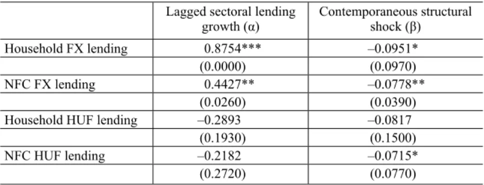
The results of these regressions can be seen in Table 2. The second column shows that the regression coefficients on the structural shock are negative and significant at the 10 percent level for each category except for household lending in HUF, i.e. an increase in capital requirement is associated with a reduction in growth in lending in the specific sectors. The lagged variables were used to simu-late whether the impact of the shock fades out over time. Although the signs are 5 See also Noss – Toffano (2014).
all positive, in line with our prior expectations, they are not significant in the case of lending in HUF either in the household or in the corporate sector.
Using these estimation results, our calculations suggest that 53% of the total decrease in lending would have materialised in foreign currency lending (both in households and the corporate sector) and 47% in HUF lending. In the foreign currency segment, lending to households would have decreased roughly equally in lending to households and corporates. In contrast with the intuitive assumption that adjustment is faster in the corporate segment, our results thus suggest that the banking sector would have reacted more intensively in the household segment.
Based on the results of the SVAR model and the above regression, Figure 12 demonstrates the alternative evolution of lending to the private sector in the most pessimistic case, i.e. where the increase in the capital requirement was considered to be a credit supply shock. It shows that even if regulatory authorities had re-acted to the increasing (FX) lending by requiring counter-cyclical capital buffer, they would have been able to only temporarily slow down the build-up of FX loans. The outstanding amount of household loans denominated in HUF and FX would have been lower by around 8% in both cases, while the reduction in corpo-rate loans denominated in HUF and FX would have been 6% for both categories at the end of the period.
Table 2. Estimation results from the regression of sectoral lending growth on the series of structural shocks
Lagged sectoral lending
growth (α) Contemporaneous structural shock (β)
Household FX lending 0.8754*** –0.0951*
(0.0000) (0.0970)
NFC FX lending 0.4427** –0.0778**
(0.0260) (0.0390)
Household HUF lending –0.2893 –0.0817
(0.1930) (0.1500)
NFC HUF lending –0.2182 –0.0715*
(0.2720) (0.0770)
Note: *, ** and *** indicate significance at the 10, 5 and 1 percent level, respectively.
Figure 11. Impulse responses of a 13 basis point shock to the change in the aggregate CAD ratio on growth of lending to different sectors
7. CONCLUSIONS
The main purpose of this paper was twofold. First, it aimed to estimate the effect of the tightening of the regulatory capital requirements on the real economy in pe-riods of credit upswing. Second, it intended to show whether applying a counter-cyclical capital buffer measure as set down in the Basel III rulescould have helped to reduce the pace of FX lending growth in Hungary, mitigating the build-up of vulnerabilities in the run-up to the GFC. In order to answer these questions, we used a VAR-based approach with the aim of understanding the impact of shocks to capital adequacy in the pre-crisis period. An increase in the regulatory capital requirement is typically considered to be a credit supply shock since it increases the funding costs of banks. However, this relationship could have changed during the recent GFC. Specifically, stricter regulations could lower funding costs by improving investor confidence.
Since the relationship between regulatory capital and lending growth is ambig-uous, we estimated two VAR models. The unconstrained version aimed to provide the upper bound for the effect of macroprudential tightening on the real economy, as the shock is not constrained to be a supply shock. Therefore, it allows for the post-crisis assumption of the changed relationship between lending and capital. In contrast with this, in the SVAR model we introduced sign restrictions on lending and alternative funding growth (negative sign for the former and positive for the latter) in line with our assumption about their pre-crisis behaviour. The results of this estimation serve as the lower bound for the possible effects on the real economy. The analysis concludes that an increase of 13 basis points in aggregate capital adequacy ratio, i.e. keeping the ratio at its 2005 Q1 level, is associated with a decline of 0–14 percentage points in cumulative real lending growth compared to actual growth after 10 quarters. Given that actual cumulative growth was 100 percent between 2004Q1 and 2007Q3, our estimation results thus indicate only a modest slowdown to 86 percent. These results have three important implications.
1. Regulatory authorities would not have been able to avoid the upswing of FX lending by requiring counter-cyclical capital bufferseven if such a tool had been available. By using this tool, they could have slowed down the in-crease in lending only temporarily. After 4 quarters, it would have regained its momentum.
2. A more pronounced tightening might have eliminated FX lending, but at the expense of real GDP growth. Macroeconomic fundamentals were fragile when FX lending started, with the significant fiscal vulnerabilities requir-ing the central bank to keep the policy rate at elevated levels. Due to the high differential between HUF and FX interest rates and households’ low risk awareness regarding exchange-rate volatility, FX lending became very
popular and contributed significantly to real GDP growth in the pre-crisis period. The bottom line is that unsustainable fiscal policy led to a trade-off between economic growth and the build-up of new vulnerabilities in the form of FX lending.
3. The results support the post-crisis conventional wisdom about the inade-quacy of pre-crisis regulatory frameworks. Therefore, it points toward pro-viding more power and flexibility to the authorities that are responsible for maintaining financial stability in order to make them capable of identifying systemic risks and acting on them in a fast and efficient manner.
REFERENCES
Admati, A. – Hellwig, M. (2013): The Bankers’ New Clothes. Princeton University Press.
Bank for International Settlements (2010): Assessing the Macroeconomic Impact of the Transition to Stronger Capital and Liquidity Requirements.Macroeconomic Assessment Group, BIS, Final Report, Basel.
Berlinger, E. – Walter, Gy. (2015): Income-Contingent Repayment Scheme for non-Performing Mortgage Loans in Hungary. Acta Oeconomica, 65(S1): 125–149.
Berrospide, J. M. – Edge, R. M. (2010): The Effects of Bank Capital on Lending: What do We Know, and What does It Mean? Federal Reserve Board, Finance and Economics Discussion Series, Washington, D.C.
Bethlendi, A. – Czeti, T. – Krekó, J. – Nagy, M. – Palotai, D. (2005): A magánszektor deviza-hitelezésének mozgatórugói (Driving Forces behind Private Sector Foreign Currency Lending in Hungary). MNB Háttértanulmányok, HT.2.
Bodnár, K. (2006): Survey Evidence on the Exchange Rate Exposure of the Hungarian SMEs. MNB Bulletin, 1(1): 6–12.
Bridges, J. – Gregory, D. – Nielsen, M. – Pezzini, S. – Radia, A. – Spaltro, M. (2014): The Impact of Capital Requirements on Bank Lending. Bank of England, Working Papers, No. 486. Brun, M. – Fraisse, H. – Thesmar, D. (2015): The Real Effects of Bank Capital Requirements.
Banque de France, Débats économiques et fi nanciers, No. 8.
Claessens, S. (2014): An Overview of Macroprudential Policy Tools. IMF Working Papers, WP/14/214.
Csajbók, A. – Hudecz, A. – Tamási, B. (2010): Foreign Currency Borrowing of Households in New EU Member States. MNB Occasional Papers, No. 87.
Enders, W. (2010): Applied Econometric Time Series. 3rd edition, John Wiley&Sons.
Fry, R. – Pagan, A. (2007): Some Issues in Using Sign Restrictions for Identifying Structural VARs. Queensland University of Technology, Brisbane, National Centre of Econometric Research (NCER), Working Paper Series, No. 14.
Fry, R. – Pagan, A. (2011): Sign Restrictions in Structural Vector Autoregressions: A Critical Re-view. Journal of Economic Literature, 49(4): 938–960.
Holló, D. (2012): Identifying Imbalances in the Hungarian Banking System (‘Early Warning’ Sys-tem). MNB Bulletin, October, 7(3): 38–45.
Hosszú, Zs. – Körmendi, Gy. – Mérő, B. (2015): Univariate and Multivariate Filters to Measure the Credit Gap. MNB Occasional Papers, OP. 118.
Hosszú, Zs. – Körmendi, Gy. – Tamási, B. – Világi, B. (2013): Impact of the Credit Supply on the Hungarian Economy. MNB Bulletin, Special Issue, October: 81–90.
IMF (2000): Macroprudential Indicators of Financial System Soundness. Occasional Paper, No. 192.
Kiss, G. – Nagy, M. – Vonnák B. (2006): Credit Growth in Central and Eastern Europe: Conver-gence or Boom? MNB Working Papers, 2006/10.
Magyar Nemzeti Bank (2009): Report on Financial Stability, April. Budapest. Magyar Nemzeti Bank (2010): Report on Financial Stability, April. Budapest. Magyar Nemzeti Bank (2012): Report on Financial Stability, April. Budapest.
Magyar Nemzeti Bank (2014): Improving Hungary’s Debt Profi le. https://www.mnb.hu/letoltes/ banks_can_contribute_to_Hungary_s_self-fi nancing_through_government_security_purchas-es_-_Background_material.pdf
Mérő, K. (2014): Macroprudential Warning in the Euro Zone and Hungary. Acta Oeconomica, 64(4): 397–417.
Modigliani, F. – Miller, M. H. (1958): The Cost of Capital, Corporation Finance and the Theory of Investment. The American Economic Review, Vol. 48.
Myers, S. – Majluf, N. (1984): Corporate Financing and Investment Decisions When Firms Have Information that Investors do not Have. NBER Working Papers, No. 1396.
Noss, J. – Toffano, P. (2014): Estimating the Impact of Changes in Aggregate Bank Capital Re-quirements during an Upswing. Bank of England, Working Papers, No. 494.
Páles, J. – Homolya, D. (2011): Developments in the Costs of External Funds of the Hungarian Banking Sector. MNB Bulletin, October, 6(3): 61–69.
Rosenberg, C. – Tirpák, M. (2008): Determinants of Foreign Currency Borrowing in the New Member States of the EU. IMF,WP/08/173.
Szombati, A. (2010): Systemic Level Impacts of Basel III on Hungary and Europe. MNB Bulletin, 5(4): 33–42.
Tamási, B. – Világi, B. (2011): Identifi cation of Credit Supply Shocks in a Bayesian SVAR Model of the Hungarian Economy. MNB Working Papers, No. 7.
Zsámboki, B. (2007): Impacts of Financial Regulation on the Cyclicality of Banks’ Capital Re-quirements and on Financial Stability. MNB Bulletin, 2(2): 47–53.