Locality-Aware Clustering Application Level Multicast for Live Streaming Services on the Internet

Locality-Aware Clustering Application Level Multicast

for Live Streaming Services on the Internet

KANCHANA SILAWARAWETAND NATAWUT NUPAIROJ

Department of Computer Engineering Chulalongkorn University Bangkok, 10300 Thailand

With the rapid growth of Internet, media streaming plays an important role for the growing demand of media service. Application Level Multicast (ALM) has emerged as a key alternative to enable broadcasting the streaming media over the Internet. Several studies have proposed solutions to construct ALM multicast trees with various aspects such as end-to-end delay optimization, quick joining delay, small maintenance join/leave overhead, and balance multicast tree. However, these approaches focus on the optimiza-tion of a simple measurement, end-to-end delay, while ignoring other factors such as bandwidth consumptions, which can be very critical for large-scale ALM. In addition, the tier-based nature of the Internet further increases the difficulties of constructing scalable ALM multicast tree. This paper proposes a hierarchical structure approach called Local-ity-Aware Clustering (LAC), which utilizes the knowledge of network topology to con-struct an efficient ALM multicast tree. Based on simulation studies, LAC algorithm can reduce the overlay stress by more than 80% comparing to traditional algorithms such as ZIGZAG and MBMT/MSMT while maintaining low overlay delay even when there are large number of nodes. This simulation results show that LAC algorithm can construct ALM multicast trees that are more localized, efficient and scalable than the traditional approaches.

Keywords: locality-aware clustering, application level multicast, landmark, bandwidth localization, bandwidth efficiency

1. INTRODUCTION

The success of live multimedia services on the Internet, such as event broadcasting, Internet TV, and Internet radio, has increased the amount of multimedia traffics drasti-cally. Many content providers adopt media streaming technology such that an end user can start watching the media as soon as the download starts. Nevertheless, these services rely on the network capability to satisfy traffic requirements such as bandwidth and jitter delay. This usually requires support from underlying network equipment.

Application Level Multicast (ALM) has emerged as a key alternative to enable broadcasting the live streaming media on the Internet without any support from network equipment. ALM typically requires an efficient and scalable structure of unicast commu-nication to support a large number of users. To be a good ALM structure for live stream-ing services, the structure has to meet two goals; (1) bandwidth efficiency, which deliver the streaming to the end-host with sufficient bandwidth that matches the requirements of the streaming application, (2) scalability, which minimize system resource usage to sus-tain the large number of users. To satisfy these goals, many ALM overlay structures, which are usually tree-based so called “multicast tree”, are proposed. Many works have

Received December 22, 2008; revised September 9, 2009; accepted November 18, 2009. Communicated by Rong-Hong Jan.

stant number is too pessimistic.

To utilize the underlying network resources effectively, several topology-aware ap-proaches have been proposed. In general, topology-aware apap-proaches, such as MSMT/ MBMT [5], have to measure all physical links in the network. This can be very imprac-tical for large-scale network such as the Internet as it is almost impossible to ping all nodes in the network and massive amount of information must be exchanged. In addi-tion, the network environment is very dynamic. Thus, the measured information can be-come obsolete very quickly and re-measurements are needed.

This paper proposes a Locality-Aware Clustering ALM (LAC) that can construct a multicast tree with good scalability, bandwidth efficiency, and practicality for live strea- ming services. To utilize the fact that the Internet spans several countries, links of the Internet are tier-based by nature as they can be classified into transit links and stub links. Hence, a good ALM approach focuses on the bandwidth localization, which is to mini-mize the bandwidth consumption on the transit links and utilize more bandwidths on the stub links. Moreover, this paper also proposes a simple geographical information called landmark to classify the links. By using landmarks, LAC can construct a multicast tree with maximum bandwidth localization and minimal latency measurements. The perform-ance of the approach is evaluated using simulation. The simulation results show that LAC algorithm demonstrates better overlay utilization and offers better scalability than other traditional ALM approaches.

The organization of this paper is as followed. Section 2 defines all necessary models, including physical model, logical model, ALM model and ALM performance metrics. Section 3 proposes Locality-Aware Clustering algorithm. This study evaluates and ana-lyzes LAC algorithm by comparing with ZIGZAG, MSMT/MBMT through simulation in section 4. Section 5 discusses the related work and finally section 6 concludes the paper.

2. MODELS AND ASSUMPTIONS

2.1 Physical Model

In general, a physical network is represented as a general graph G = (V, E), where V denotes a set of nodes and E denotes a set of physical links. A node in physical network, vi, can be either a host or a router. For a physical link e(vi, vj) ∈E, which is a link

by d(e(vi, vj)) and bw(e(vi, vj)), respectively. Let the application bandwidth, denoted by abw(e(vi, vj)), to be the bandwidth that an application uses for transmitting data over a

physical link e(vi, vj), including all duplicated packets on that particular link. The

utiliza-tion of a link, denoted by u(e(vi, vj)), is ratio of application bandwidth and the link

band-width. Thus, ( ( , )) ( ( , )) . ( ( , )) i j i j i j abw e v v u e v v bw e v v = (1)

Typically, the effectiveness of a streaming application is usually limited by the bot-tleneck link, which is the link being utilized the most. The botbot-tleneck link, denoted by BL, is the link with maximum utilization. In this case,

( , ) ( ) max { ( ( , ))}. j i i j e v v E u BL u e v v ∈ = (2)

In reality, Internet is the networks of networks. Thus, it exhibits the characteristics of the tier-based environment [7], such as domestic tier and international tier. Therefore, to represent the real network such as Internet, this paper will extend the physical network model with transit-stub architecture [8]. This architecture consists of two domain catego-ries, Transit-Domain (TD) and Stub-Domain (SD). Transit-domain is consisting of inter-national-level Transit-Nodes (TN) acting as connection points between transit-nodes and stub-domains. Thus, the transit-domain provides Internet backbone to connect between the two transit-nodes, as well as, between a transit-node to stub-domains via transit link or inter-area link. For stub-domain, all nodes in the same domain are assumed to be in near- by physical location or area. Thus, these nodes communicate other nodes in the same stub-domain via stub links. In this study, the data traffics within a stub-domain are called stub traffic and the traffics within the transit-domain or between a transit-node and stub- domain are called transit traffic.

The extended model for a physical network G = (V, E) is formally defined as fol-lowed. Suppose the network has n stub-domains. Let ai be a stub-domain and Vi be a set

of nodes in ai. V0 is defined as the set of transit nodes. The set of nodes V can be

parti-tioned into n subsets, = =1 . n i i

V ∪ V In addition, a set of all links E composes of a set of transit links Et, which is the collection of links connecting transit-nodes with other transit

nodes or stub-domains, and a set of stub links Es, which is the collection of links

con-necting nodes in the same stub-domains. Then, the set of link E is Et∪Es. Suppose et is a

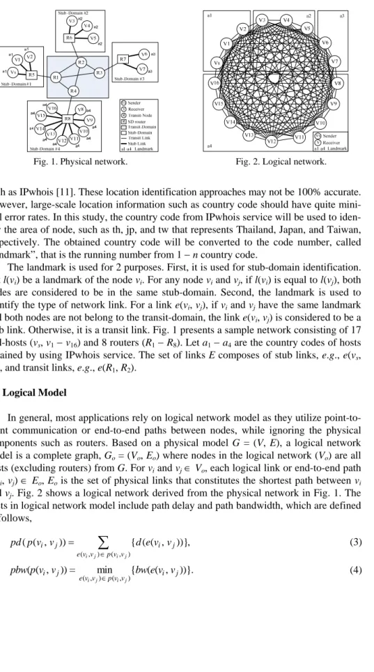
transit link and es is a stub link. This works make general assumptions that bw(et) < bw(es). Fig. 1 shows an example of Internet transit-stub architecture with 4 stub-domains

and one transit-domain.

Based on this model, nodes and links in physical topology will be classified into transit-domain and stub-domain. This process requires the measuring of node information such as delay and bandwidth using many popular tools such as traceroute, pathchar [9], Max-Delta [10]. However, these approaches usually take long time to measure the infor-mation, require frequent measurement, and consume a lot of resources. To simplify the identification process, this study utilizes the fact that nodes in the same domain should be in the nearby geographical area. Thus, area identification can be done easily such as ask-ing user to provide the area information or inquirask-ing from some standard Internet services

Fig. 1. Physical network. Fig. 2. Logical network.

such as IPwhois [11]. These location identification approaches may not be 100% accurate. However, large-scale location information such as country code should have quite mini-mal error rates. In this study, the country code from IPwhois service will be used to iden-tify the area of node, such as th, jp, and tw that represents Thailand, Japan, and Taiwan, respectively. The obtained country code will be converted to the code number, called “landmark”, that is the running number from 1 −n country code.

The landmark is used for 2 purposes. First, it is used for stub-domain identification. Let l(vi) be a landmark of the node vi. For any node vi and vj, if l(vi) is equal to l(vj), both

nodes are considered to be in the same stub-domain. Second, the landmark is used to identify the type of network link. For a link e(vi, vj), if vi and vj have the same landmark

and both nodes are not belong to the transit-domain, the link e(vi, vj) is considered to be a

stub link. Otherwise, it is a transit link. Fig. 1 presents a sample network consisting of 17 end-hosts (vs, v1−v16) and 8 routers (R1−R8). Let a1−a4 are the country codes of hosts

obtained by using IPwhois service. The set of links E composes of stub links, e.g., e(vs, R5), and transit links, e.g., e(R1, R2).

2.2 Logical Model

In general, most applications rely on logical network model as they utilize point-to- point communication or end-to-end paths between nodes, while ignoring the physical components such as routers. Based on a physical model G = (V, E), a logical network model is a complete graph, Go = (Vo, Eo) where nodes in the logical network (Vo) are all

hosts (excluding routers) from G. For vi and vj∈Vo, each logical link or end-to-end path p(vi, vj) ∈Eo, Eo is the set of physical links that constitutes the shortest path between vi

and vj. Fig. 2 shows a logical network derived from the physical network in Fig. 1. The

costs in logical network model include path delay and path bandwidth, which are defined as follows, ( , ) ( , ) ( ( , )) { ( ( , ))}, i j i j i j i j e v v p v v pd p v v d e v v ∈ =

∑

Fig. 3. Packet flow of IP multicast. Fig. 4. Packet flow of ALM.

2.3 Application Level Multicast Model

Streaming applications often require multicast services for delivering their stream-ing feeds. Typically, multicast services for streamstream-ing can be based on either IP multi-casting or Application Level Multimulti-casting (ALM). The main concept of ALM is to im-plement the multicast service at the application level. At this level, ALM utilizes point- to-point communication to create overlay network atop of logical network model. This enables ALM to become independent from physical network topology. Note that this study focuses on the ALM with single source. Thus, the ALM structure in this study is assumed to be based on tree.

Figs. 3 and 4 show the differences between IP multicast and ALM. The arrow dash lines represent the packet flows on the transit link, while the arrow dot lines represent the packet flows on the stub link. Obviously, IP multicast mechanism relies on the routers to forward data packets from the sender to receivers without duplication. On the contrary, ALM utilizes unicasts to deliver packets. Thus, some unicasts may share the same physi-cal link. This can lead to multiple sending of the same packet over this link, physi-called link stress. The link stress of a physical link e(vi, vj), denoted by st(e(vi, vj)), refers to the number

of duplicated packets on that link. This paper defines the stress on transit link to be the maximum stress of all transit links on the multicast tree. The stress on stub stress is the maximum stress of all stub links, and the overlay stress is the maximum stress of all links.

Given an ALM tree, T = (Go, vs, D, S). Let Go be a logical network model. Let vs be

the source which is the root of the tree and let D be the set of nodes in Go which are the

destinations of ALM traffic. Streaming data traffic from the source to all destinations may require multiple unicasts. For a destination vi∈D, a streaming path s(vs, vi) constitutes

the path between vs and vi. SPis the set of all streaming paths in the tree. Streaming path

delay and streaming path bandwidth are defined as followed. The streaming path delay, denoted by sd(s(vs, vi)), is the sum of end-to-end delay of the logical link along the

streaming path. The streaming path bandwidth, denoted by sbw(s(vs, vi)), is the minimum

path bandwidth on the streaming path. Thus:

( , ) ( , ) ( ( , )) { ( ( , ))}, s i s i s i s i p v v s v v sd s v v pd p v v ∈ =

∑

Fig. 5. Overlay network. Fig. 6. The relationship of the three models.

Fig. 5 presents the overlay network of the ALM tree in Fig. 4. To perform multicasting, vs establishes unicast connections to v1, v3, v6, v7, and v16. After the nodes receive the data,

they forward the data to other members, such as v1 to v2 and v3 to v4. The stress on transit link and stub link are 4 and 2, respectively. Finally, the overlay stress is 4.

In the overlay network, the overlay delay, denoted by od(T), is the maximum strea- ming path delay comparing to all of them on the overlay network. The overlay bandwidth, denoted by obw(T), is the minimum streaming path bandwidth of the overlay network. Thus, ( , ) ( ) max { ( ( , ))}, s i s i s v v SP od T sd s v v ∈ = (7) ( , ) ( ) max { ( ( , ))}. s i s i s v v SP obw T sbw s v v ∈ = (8)

Fig. 6 summarizes the relationships between the Physical model, the Logical model, and the ALM model. Some ALM algorithms base entirely on physical model, while some others focus only on logical model. With the introduction of landmark in the ex-tended physical model, LAC algorithm can utilize both physical model and logical model to construct ALM trees with good performance. ALM performance matrices are dis-cussed in the next section.

2.4 ALM Performance Metrics

To evaluate the effectiveness of ALM on the Internet, this study uses the following metrics: link stress, overlay utilization, transit byte ratio, and overlay delay. The defini-tions of these metrics are as follows,

1. Link stress: This metric measures the quantity of the flooding packets. To utilize net-work bandwidth effectively, the stress must be minimized, especially at the link with small bandwidth like a transit link and highly-congestion link like a bottleneck link. The transit stress, denoted by stt, and the bottleneck link stress, denoted by stb, are

( ,imax { ( ( ,j) t ))}, t i j e v v E st st e v v ∈ = (9) (max { ( () ))}. b e BL E st st e BL ∈ = (10)

2. Overlay utilization: As mentioned earlier, the bottleneck link is very critical to the streaming application. Thus, the utilization of the bottleneck link is used to represent the overlay utilization. Therefore,

u(T) = u(BL). (11)

3. Transit byte ratio: This metric is a metric that shows the quality of localization-aware. It is used to quantify the quality of traffic localization by considering traffic in the stub links. The transit byte ratio, tbr, is the ratio of total bytes, tb, on the transit links by to-tal bytes of all links.

( , ) ( , ) { ( ( , ))} ( ) { ( ( , ))} i j t i j i j e v v E i j e v v E tb e v v tbr T tb e v v ∈ ∈ =

∑

∑

For good localization, the ALM should avoid using the transit links. Thus the transit byte ratio should be closer to 0. In addition, the stub byte ratio, denoted sbr(T), is de-fined as follows,

sbr(T) = 1 −tbr(T). (13)

4. Overlay delay: This metric is the maximum streaming path delay in the ALM tree. In this assumption, the overlay delay is not quite critical for the live streaming services. The delay just has to be within the pre-defined bound. Hence, the overlay delay is not the main metric in this evaluation.

3. LOCALITY-AWARE CLUSTERING (LAC)

In this section, a new algorithm called Locality-Aware Clustering (LAC) is proposed to construct an efficient overlay tree for live streaming over the Internet. LAC algorithm uses landmark information to partition nodes and links into groups and constructs the overlay tree accordingly.

3.1 Locality-Aware Clustering Hierarchical Structure

Traditionally, ALM overlay trees are constructed based on the optimization of the overlay delay. This may be significant in some ALM applications such as network game and video conference [12]. In some other applications such as live streaming, some de-lays within bound are usually acceptable and scalability becomes an important issue as it needs to support large number of audiences. To solve this problem, a new algorithm called

node is also a member of the parent cluster. For the top cluster, the source or the root of the tree acts as both header node and distributor node.

2. Distributor Node (DNi): DNi is responsible for receiving streaming feed from the HN

of this cluster and distributing data to other members of the cluster. DN also maintains the membership of the cluster. In addition, DN is the backup of HN. Thus, when HN fails, DN will become HN and a new DN is elected from one of the members.

3. Other node (ON): The rests of members are called the Other Nodes (ONs), which are the children of DN. ONs receive data from DN. If the cluster has child clusters, HNs of the child clusters are also ONs of this cluster. In addition, we define {ON}i to be a set

of all ONs in Ci.

Fig. 7 shows an example of an LAC tree that generate from the physical network in Fig. 1. The tree has three overlapped clusters, C0, C1, and C2. C0 is the root cluster, which also includes the source and the root node (vs). vs acts as both HN0 and DN0 of C0 and v8 is the only ON in this cluster. In C1, there are three members (vs, v1, and v2). vs is an HN1, v1 is the DN1, and v2 is the only ON. In C2, the HN2 is v8, the DN2 is v9, and v10, v12, v16, v3, v5 are the members of {ON}2. Based on the structure, the streaming feed comes from the source node vs to its only child in C0, v8. Upon receiving data, v8 as HN2 forwards the streaming feed to DN2 (v9), which forwards the feed to all {ON}2. In addition, acting as HN1, vs also forwards its data to v1, which is DN1.

Although, LAC structure is based on ZIGZAG and NICE, LAC structure is more efficient because it combines the information from physical model and logical model to implement the traffic localization concept called “Locality-Aware”. This concept bases on the fact that the communication between two nodes within the same stub domain should be more efficient than those across two different domains. Thus, the concept fo-cuses on constructing a cluster such that stub links (or local links) are preferred over tran-

V1 V8 V12 V9 V10 V16 V3 V5 HN2 HN1 DN2 ON2 DN1 a4 a4 a1 a1 a4 a4 a4 a2 a2 V2 ON1 a1 Vs C1 C2 HN: Header Node DN: Distributor Node ON: Other Node Vs: Sender

a1- a4: Landmark

C0

HN0, DN0 ON0

sit links as intra-cluster links. This minimizes the stresses in the transit links, which lead to better performance and greater scalability. Considering the LAC structure, DN has to communicate with many ONs. If DN and ON are on the same physical area, they can communicate directly via stub links. With this concept, LAC algorithm tries to group nodes with the same landmark into the same cluster. This will be done when a new node joins the tree.

3.2 Joining a New Node

To join a new node, LAC joining algorithm, presented in Fig. 8, is used to find the target cluster. Based on the localization, LAC joining algorithm selects the target cluster (Cx) by keeping nodes in the same area within the same cluster. Suppose a new node vi

want to join the structure. If the vi is the source node, it becomes the root of LAC

multi-cast tree. Otherwise, vi will requests all DN list and their landmarks from the DN of the

root cluster (DN0) to construct a shortlist of the near-by clusters. A near-by cluster is a cluster that shares the same landmark with vi. If there are more than one cluster in the

near-by cluster shortlist, vi will select the Cx which is not full and has the smallest latency.

Note that if all clusters in the shortlist are full, vi will select the Cx based on the latency

only. If the near-by cluster shortlist is empty, vi measures the latency from vi to all DNs in

the multicast tree and joins the cluster with the smallest latency.

The algorithm of LAC: Joining new node 1. If (source(vi)) 2. root = vi 3. else 4. if (#C == 0) 5. HN0 = DN0 = root 6. else DNx = FindCx(vi, l(vi)) 7. end if 8. JoinNode(DNx, vi, pd(DNx, vi)) 9. if (#Member(Cx) > 9) 10. SplittingAndMerging(Cx) 11. end if 12. end if

Fig. 8. The algorithm of joining newcomer.

When the target cluster is selected, vi joins as a child of the DN of the target cluster.

LAC joining algorithm then evaluates the size of the cluster. If the cluster is too large (more than 3k), the cluster is partitioned by splitting and merging algorithm.

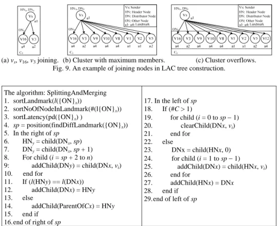
Fig. 9 shows an example of joining nodes to the multicast tree. Suppose the multi-cast tree already has 3 nodes, as demonstrated in Fig. 9 (a), and there are 7 new nodes, v9, v10, v8, v1, v2, v5, and v12, want to join the multicast tree. When the first 6 nodes join the multicast tree, all nodes will join the root cluster, C0, as presented in Fig. 9 (b). When v12 joins the multicast tree in Fig. 9 (c), the root cluster becomes overflow as its size is 10 (including the root node), which is more than 3k (k = 3). In this case, the cluster will be partitioned into 2 clusters by calling SplittingAndMerging in line 10.

2. sortNoOfNodeInLandmark(#(l{ON}x)) 3. sortLatency(pd({ON}x) ) 4. sp = position(findDiffLandmark({ON}x)) 5. In the right of sp 6. HNy = child(DNx, sp) 7. DNy = child(DNx, sp + 1) 8. For child (i = sp + 2 to n) 9: addChild(DNy) = child(DNx, vi) 10. end for 11. If (l(HNy) == l(DNx)) 12. addChild(DNx) = HNy 13. else 14. addChild(ParentOfCx) = HNy 15. end if 16. end of right of sp 18. If (#C > 1) 19. for child (i = 0 to sp− 1) 20. clearChild(DNx, vi) 21. end for 22. else 23. DNx = child(HNx, 0) 24. for child (i = 1 to sp− 1) 25. addChild(DNx) = child(HNx, vi) 26. end for 27. addChild(HNx) = DNx 28. end if 29. end of left of sp

Fig. 10. The algorithm of SplittingAndMerging.

When the cluster is too large, there are two stages of the SplittingAndMerging pro-cedure. (1) Splitting the overflow cluster into two clusters, and (2) merging the new clus-ter to the multicast tree. Fig. 10 shows the detail of SplittingAndMerging algorithm.

Suppose Cx is too large. Splitting Cx will perform in 3 steps, sorting the {ON}x,

which is the set of all ONs of Cx (lines 1-3), finding the splitting position to form a new

cluster (called sp, line 4), and selecting the HN and DN for the new cluster (lines 6-7, 23). In the sorting stage, LAC first group {ON}x by their landmarks, then sort the group

of landmark by the number of nodes in decreasing order, and finally re-sort these nodes in any landmark by latency in increasing order. Note that the group of ONs with the same landmark of DNx will stay on the left side of the list. Then the splitting position is

assigned by choosing the first child, whose landmark is different from the others. If all children have the same landmark, the cluster is split in halves. Using the splitting posi-tion, HNx, DNx, and all ONs on the left side of the splitting position remain in Cx. In this

case, HNx and DNx remain unchanged. The ONs on the right side of the list will form a

new cluster, Cy. The first two nodes in the right side of the list will be chosen as new

HNy and the DNy. To prevent the new cluster from being too small, the splitting position

must be in between the third and the sixth child of the list.

To complete the process, Cy will be merged to the multicast tree using the merging

landmark of the DNx. If the both landmark are the same, the HNy will join Cx and

be-come the child of the DNx. Otherwise, the HNy will become a child of the parent cluster

of Cx. In this case, Cx and Cy become siblings. Once merged, if the parent cluster

be-comes overflow, the parent cluster will be split and merged in similar fashion.

There is a special case when splitting the root cluster, C0. Since the C0 is the root cluster, it has no parent cluster. In this case, all clusters in the multicast tree will be re- arranged by renaming all clusters and creating a new C0. Suppose the C0 is full. It will be split C0 and form C1 similar to normal splitting process. Note that the root node still re-mains as HN0 and DN0. After splitting, the tree must be re-arranged. To re-arrange the tree, the names of all clusters in the multicast tree will be increased by one. Thus, C0 be-comes C1, etc. A new C0 is created from the HN1 (after being renamed), or the root node, and the HN2 (after being renamed). For the new C0, the root node will become the HN0 and DN0 and the HN2 will become the only ON of C0.

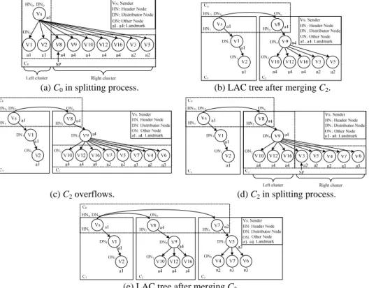
Fig. 11 shows the example of splitting and merging cluster. Fig. 11 (a) shows C0 af-ter the {ON}0 are sorted by their landmarks, number of nodes in each landmark, and la-tencies. Then the ONs will form a list in order to choose the splitting position. In C0, the first position that the landmarks are different is the third position, so the splitting position of this cluster is the node v8. Thus, the C0 is split. HN0 and DN0 (vs), as well as, all ONs

from the left side of the splitting position {v1, v2} remain in C0. HN0 and DN0 remain un-changed. The remaining ONs ({v8, v9, v10, v12, v16, v3, v5}) form a new cluster C1. The first

(a) C0 in splitting process. (b) LAC tree after merging C2.

(c) C2 overflows. (d) C2 in splitting process.

(e) LAC tree after merging C3.

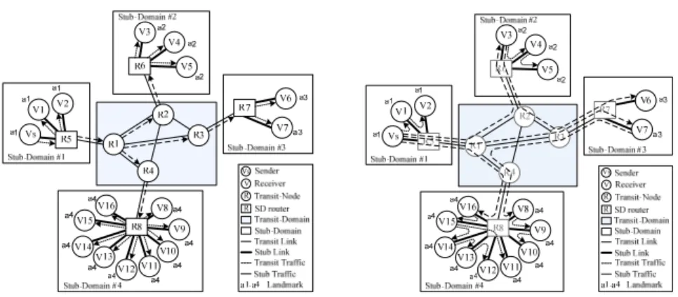
Fig. 12. ALM with locality-aware. Fig. 13. Overlay network.

two nodes in the list, v8 and v9, are chosen as the HN1 and the DN1, respectively. Since the C0 is split, all clusters in the multicast tree must be re-arranged. C0 is renamed to be C1. C1 is renamed to be C2. A new C0 is created from HN1 (vs) and HN2 (v8). The root node becomes HN of the new C0.

Similarly, Fig. 11 (c) shows LAC tree after v7, v4, and v6 join the C2 and then the cluster is overflow. C2 is partitioned into C2 ({v8, v9, v10, v12, v16}), C3 ({v3, v5, v4, v7, v6}) as illustrated in Fig. 11 (d). The new cluster C3 is merged to the multicast tree and HN3 becomes a child of C0, which is also the parent cluster of C2 in Fig. 11 (e).

Finally, Figs. 12 and 13 show an example multicast tree generated by LAC algo-rithm. Using localization strategy, LAC tree is constructed such that most streaming traf-fics have been transmitted over the stub links leading to fewer stresses in the transit links. In this example, the transit stress of this tree is 2, which is lower than the transit stresses of the tree generated by ZIGZAG in Fig. 5.

3.4 Leaving Node

There are two possible cases of node leaving the multicast tree, voluntary and in-voluntary (e.g. node crashes). When a node leaves voluntarily from a cluster in LAC tree, the leaving process is invoked. By considering the type of the leaving node, there are three cases:

1. If the leaving node is the HN of the cluster, the DN of that cluster is promoted to be a new HN. The ON node with the shortest latency from the new HN will become the new DN. 2. If the leaving node is the DN of the cluster, the ON node with the shortest latency

from the existing HN will become the new DN. 3. If the leaving node is the ON, no action is necessary.

After node leaves from the cluster, if the cluster size is not between k and 3k, all nodes in the cluster must join a cluster whose HN has the same landmark as the HN of the under- size cluster. After joining, the joined cluster may be split again if the cluster size is overflow.

In the case that a node crashes, if the crashed node is an ON, this will not affect the leaving process. If the crashed node is either HN or DN, however, part of the multicast

tree is disconnected. To prevent this problem, a heart-beat mechanism must be imple- mented between HN and DN. Once a crash is detected, the leaving process is invoked, similarly to a node leaves voluntarily.

3.5 Practical Issues

To implement LAC algorithm, node’s memory requirement, clustering time, and packet loss must be considered. In LAC algorithm, cluster information during normal operation is distributed among clusters. In this case, HN and DN must maintain the in-formation of their own cluster. Since cluster size is limited to 3k, the memory require-ments of maintaining cluster information during normal operation is quite minimal. Mem-ory requirements during clustering time, however, require special consideration. In gen-eral, node’s memory requirement and clustering time are quite related, especially during the joining period. In LAC algorithm, the time consuming step of the joining process is to construct a shortlist of near-by clusters. This requires examining the landmark infor-mation of DN of each cluster starting from the root cluster and goes further down in the multicast tree. To shorten this construction process, high-level nodes such as the root node and HN of the high-level clusters may cache cluster information of their child clus-ters. Since only landmark information of each DN is needed to represent each cluster, caching child clusters’ information for shortlist construction is not memory-demanding.

Packet loss is possible during the leaving process. For voluntarily leaving, the leav-ing node will not leave right away. It will wait until the leavleav-ing process is complete and then actually leave. For involuntarily leaving, the leaving node is crashed. Thus, it cannot wait until the leaving process is complete. In this case, other nodes in the cluster will be disconnected from the multicast tree and the streaming service is interrupted. To mini-mize the length of interruption period, the heart-beat mechanism between HN and DN must be frequent enough in order to detect the crash as soon as possible.

The other practical issue is the accuracy of location identification. Using country code as a landmark may not always be accurate as the IPWhois service may return a country code that is not corresponding to the actual location where the node is located. The inaccurate landmark information can lead LAC to construct an inefficient multicast tree. However, since the landmark is based on a country code, which is very large-scale, it is very unlikely that this information is incorrect. In addition, LAC algorithm has been designed such that it can tolerate this problem because latency is also considered during the joining process. If the landmark is incorrect, the DN that is claimed to be in the same area of the joining node will have longer latency than other DNs in the shortlist whose landmark are correct. Thus, the joining node will choose to join the DN with shorter la-tency, which should have a correct landmark. At the worst, LAC will perform as good as other cluster-based algorithms such as NICE and ZIGZAG if the inaccuracy rate is too high.

4. PERFORMANCE EVALUATION

4.1 Simulation Environment

To evaluate LAC algorithm, simulations using NS2 simulator are conducted. The physical network topologies in all simulations are randomly generated based on the

tran-Table 1 lists the parameters and their values being used in this simulation. The band- width distribution and end-to-end latency are the measurement results of [13]. The Band-width distribution is randomly assigned between 80 to 100 Mbps for stub link and 8 to 10 Mbps for transit link. All cluster size is limited at 3k where k = 3. Each streaming is 5 sec. long, and the streaming rate is 250 Kbps, which is quite typical for both audio and video streaming applications. Average values of simulating ALM trees on three different physic-cal topologies are being used in all performance comparison.

4.2 Simulation Results

As discussed in section 2.4, stress is considered the most important metric for evalu-ating ALM. To achieve good scalability on the Internet, stress in the transit links must be minimized.

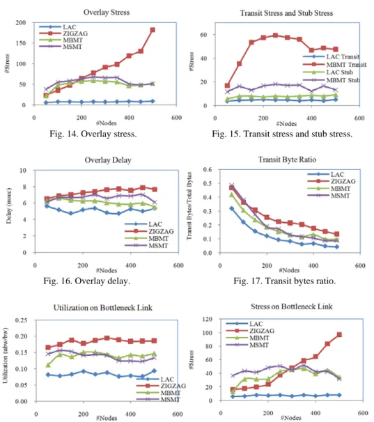
Fig. 14 shows the overlay stresses of all algorithms with different number of nodes. For ALM trees with 500 nodes, the overlay stress of ZIGZAG, MSMT/MBMT, and LAC, are 182, 52, and 9, respectively. The result shows that LAC performs quite well, especially when the number of nodes is large. LAC trees can out-perform ZIGZAG and MBMT/ MSMT by 95% and 82%, respectively. Fig. 15 compares the stresses in the transit links and in the stub links of ALM trees generated by LAC and MBMT algorithms. With lo-calization strategy, LAC tries to utilize the stub links as much as possible. Thus, the stres- ses in transit links of LAC tree remain quite low. On the contrary, the stresses in the tran-sit links of MBMT increase as ALM tree becomes larger. This is because MBMT first uses a latency-oriented spanning tree as a basis to construct an ALM tree. Then, MBMT uses link utilization as criteria to optimize the tree. With this approach, the ALM trees constructed by MBMT are basically latency-optimized, which may not be stress-opti-mized. To provide a clear explanation, let’s consider a simple example. In an MBMT tree, suppose a node vi is a parent of 3 other nodes. And suppose these 3 nodes are in the same

area and vi belongs to the different area. Since all 3 nodes are in the same area, the

laten-cies between these nodes and vi should be almost the same. Thus, for a spanning tree,

these 3 nodes will link to the same parent, vi. In this case, the connections between parent

and all 3 children will be over the same transit link, which lead to more stresses in the transit link. On the contrary, LAC will group these 3 nodes into the same cluster and have only one node connecting to vi. In this case, the transit stress is minimized.

Fig. 14. Overlay stress. Fig. 15. Transit stress and stub stress.

Fig. 16. Overlay delay. Fig. 17. Transit bytes ratio.

Fig. 18. Overlay utilization on bottleneck link. Fig. 19. Stress on bottleneck link. Fig. 16 shows the overlay delay. The results indicate that the overlay delay of LAC tree is less than the overlay delay of other trees in almost all of network sizes. Since LAC relies on the stub links, which have much lower latency than transit links, the overlay delay of LAC scheme is minimized. Fig. 17 shows the transit byte ratio as number of nodes change. The results confirm the characteristics of LAC algorithm that it utilizes the stub links more than the transit links. Comparing to other algorithms, LAC has the low-est transit bytes ratio, 0.043, while ZIGZAG has the larglow-est transit byte ratio, 0.134. This means less data is transferred on the transit links of LAC tree. Thus, with the same num-ber of nodes in the multicast tree, LAC is the most bandwidth efficient.

Fig. 18 investigates the scalability of the ALM tree on the Internet by evaluating the overlay utilization on the bottleneck link. This results show the performance of ALM tree

5. RELATED WORK

Various ALM overlay construction have been proposed for streaming services [1-6]. They can be classified into two categories, tree-based (ZIGZAG [1], STAG [3], MSMT/ MBMT [5], and NICE [6]), and mesh based (IOO [2] and SHM [4]). IOO [2] proposed an inter-overlay optimization scheme using mesh-based structure aiming for constructing efficient paths for different overlay, guaranteeing streaming service quality, and improving resource utilization. SHM [4] constructs the hierarchical structure that composes of Ren- dezvous Point (RP) and domain. The structure is a global share tree based on IP Multicast Island that does not require extra detection mechanism between end-host during the mem-ber join.

Some structures [1, 3, 5, 6] construct multicast trees using the underlying network information such as delay, bandwidth, and location information. These algorithms are considered topology-aware. STAG [3] proposed a tree construction that uses transit-stub network topology on top of physical network. This mechanism minimizes the overhead of the joining process, has low relative delay penalty, and reduce link stress. As this algo-rithm focuses mainly on latency, it is not bandwidth efficient. NICE [6] and ZIGZAG [1] construct a hierarchical cluster of nodes with each cluster having a “head” represent in the higher layer. In these algorithms, nodes are being grouped into a cluster to reduce the control overhead and allow fast joining process. NICE was designed to support network architecture with limited bandwidth. Its cluster size is bounded by a constant to avoid the bottleneck at the distributor. ZIGZAG is an extension of NICE with two additional tech-niques, cluster size balancing and capacity-based switching. It aims to minimize the over- heads during joining and leaving processes, as well as, reducing the number of network hops. However, ZIGZAG assumes all nodes are similar in term of latency and bandwidth availability. Unfortunately, this is not applicable for the Internet.

MSMT/MBMT [5] optimizes ALM tree based on the underlying network topology. Using complete information of network topology, the algorithm focuses on minimizing stress in any link and generates an ALM tree with high tree bandwidth and low link stress with low penalty in end-to-end delay. However, obtaining information required by MSMT/ MBMT, complete network topology, is not quite practical.

6. CONCLUSION

Internet, called Locality-Aware Clustering or LAC. Based on the assumption of tier-based networking structure, LAC combines the physical model and logical model to construct an efficient ALM structure for the Internet using landmark and end-to-end delay. This paper evaluates the performance of LAC scheme by comparing with ZIGZAG, MSMT/ MBMT using simulation. The experimental results clearly show that LAC tree can out- perform all other algorithms by more than 80% when comparing overlay stress and by more than 30% when comparing the utilization on bottleneck link. In addition, the over-lay deover-lay of LAC tree is minimal. The simulation results also indicate that the effective-ness of LAC mechanism is due to its localization strategy as LAC relies on the stub tier, which can greatly reduce the bandwidth requirements on the transit tier, whose band-width is usually quite limited. Therefore, LAC algorithm can generate a bandband-width-effi- cient ALM structure with low latency and good scalability for live streaming. The future works will extend LAC algorithm to support multiple source services.

REFERENCES

1. D. A. Tran, K. A. Hua, and T. T. Do, “ZIGZAG: An efficient peer-to-peer scheme for media streaming,” in Proceedings of International Conference on Computer Com-munications, 2003, pp. 1283-1292.

2. X. Liao, H. Jin, Y. Liu, and L. M. Ni, “Scalable live streaming service based on in-ter-overlay optimization,” IEEE Transactions on Parallel and Distributed Systems, 2007, pp. 1663-1674.

3. J. Cui, Y. He, and L. Wu, “More efficient mechanism of topology-aware overlay construction in application-layer multicast,” in Proceedings of International Con-ference on Networking, Architecture, and Storage, 2007, pp. 31-36.

4. S. Lu, J. Wang, G. Yang, and C. Guo, “SHM: Scalable and backbone topology-aware hybrid multicast,” in Proceedings of IEEE Conference on Computer Communica-tions and Networks, 2007, pp. 699-703.

5. X. Jin, W. P. K. Yiu, S. H. G. Chan, and Y. Wang, “On maximizing tree bandwidth for topology-aware peer-to-peer streaming,” IEEE Transactions on Multimedia, Vol. 9, 2007, pp. 1580-1592.

6. S. Banerjee, B. Bhattacharjee, and C. Kommareddy, “Scalable application layer mul-ticast,” in Proceedings of ACM SIGCOMM, 2002, pp. 205-217.

7. H. Haddadi, M. Rio, G. Iannaccone, A. Moore, and R. Mortier, “Network topologies: inference, modeling, and generation,” IEEE Communications Surveys and Tutorials, Vol. 10, 2008, pp. 48-69.

8. E. W. Zegura, K. Calvert, and S. Bhattacharjee, “How to model an Internetwork,” in Proceedings of IEEE Conference on Computer Communication, 1996, pp. 594-602. 9. V. Jacobson, Pathchar, http://www.caida.org/tools/utilities/others/pathchar/.

10. X. Jin, W. P. K. Yiu, S. H. G. Chan, and Y. Wang, “Network topology inference based on end-to-end measurements,” IEEEJournal on Selected Areas in Communi-cations, Vol. 24, 2006, pp. 2182-2195.

11. The APNIC Whois Database, http://wq.apnic.net/apnic-bin/whois.pl.

12. S. Hajime, S. Hiroki, and T. Yoshito, “P2P grouping for the delay sensitive applica-tions,” IEIC Technical Report, Vol. 106, 2006, pp. 13-18.

Ph.D. degree in Computer Engineering at Chulalongkorn Univer-sity. Her research interests include multicast, parallel and distrib-uted computing, and grid computing.

Natawut Nupairoj received the B.E. in Computer Engineer-ing from Chulalongkorn University in 1990, M.S. and Ph.D. in Computer Science from Michigan State University in 1993 and 1998, respectively. Since 1998, he has been a Lecturer at Depart- ment of Computer Engineering, Chulalongkorn University. His research interests include grid computing, distributed system, and service oriented architecture.