A Simple Model for Credit Migration and Spread Curves

A Simple Model for

Credit Migration and Spread Curves

Li Chen

_{Damir Filipovi´c}

May 14, 2003

Abstract

We propose and examine a simple model for credit migration and spread curves of a single firm both under the real-world and the risk-neutral measure. This model is a hybrid of a structural and a reduced-form model. Default is triggered either by successive downgradings of the firm or an unpredictable jump of the state process. The default time is accordingly decomposed into predictable and totally inaccessible part.

1

Introduction

We propose and examine a simple model for credit migration and spread curves of a single firm both under the real-world and the risk-neutral measure. This model is based on an affine state process Y = (Y1_{, Y}2_{, Y}3_{) taking values in}

R3

+ =R3+∪∆ which is the one-point compactification ofR3+={x∈R3|xi≥0}

(∆ is the “point at infinity”). The pair (Y2

t, Yt3) represents the state of the firm, where Y3 is a simple

point process with Y3

0 = 0 and jump size 1 whose intensity depends linearly

on Y2_{. While Y}3 _{takes account of the unpredictable credit event (default),}

Y2 _{is a credit index of the firm ranging in the non-negative real numbers with}

Y2

t = 0 corresponding to the best credit rating (e.g. Aaa) andYt2= +∞(that

is,Yt= ∆) meaning default.

The firm has defaulted by timetif

Yt∈ D:={∆} ∪ {y∈R3+|y3>0},

which is an absorbing state. Hence a default of the firm is triggered either by i) successive downgradings (explosion ofY2_{) or ii) an unpredictable jump ofY}3_.

The combination of i) and ii) yields a decomposition of the firm’s default time TD := inf{t|Yt∈ D}=T∆∧TJ

∗_{Information Sciences and Systems, Princeton University.}

†_{Operations Research and Financial Engineering, Princeton University, Princeton, NJ} 08544, USA. Email Contacts:{lichen, dfilipov}@princeton.edu

into a predictable and a totally inaccessible part where T∆:= inf{t|Yt= ∆}

is the explosion time ofY and

TJ:= inf{t|Yt3= 1}

is the first jump time ofY3_.

The actual credit rating (e.g. Moody’s) can in principle be obtained by a monotone transformation ofY2

t. That is,R+ is decomposed into finitely many

non-overlapping intervalsIAaa, IAa, . . . withYt2∈IR meaning that the firm is

R-rated,R∈ {Aaa, Aa, . . .}, given thatY3

t = 0.

The componentY1_{describes the short ratesrup toT}

∆. The processritself

follows a Cox–Ingersoll–Ross [5] (CIR) model. Our setup allows for dependence of interest rates and credit migration.

Due to the affine nature of Y and r we find explicit expressions for the real-world default probabilities and corporate bond prices. The resulting zero-recovery yield spread curve is affine inY. The change from real-world to risk-neutral measure is specified by the market risk premium (r-dynamics) which implicitly affects the characteristics of the credit risk (Y-dynamics).

Our approach constitutes a hybrid of a structural and a reduced-form de-fault time model. Here, with “structural” we associate any dede-fault time model which is based on the (predictable) first passage time of an underlying eco-nomic factor process, see e.g. [6, 11, 16]. The “reduced-form” on the other hand stands for any intensity based model of a (totally inaccessible) default time, see e.g. [17, 18]. We refer to [1, 12] for a recent overview of credit risk models and a comprehensive reference list. The novelty of our model lies in its explicit and tractable structure. An extension towards multi-firm models with default correlation and counterparty risk is given in [3].

The remainder of the paper is as follows. In Section 2 we introduce the basic affine state process Y and discuss some of its properties, citing results from [9]. In Section 3 an explicit expression for the real-world default probabilities is derived. In Section 4 we obtain expressions for treasury and corporate bond prices, with zero-recovery and fractional recovery at maturity. The zero-recovery yield spread curve is given as an explicit affine function of Y (Lemma 4.2). Section 5 provides an equivalent change of measure which links the real-world and the risk-neutral model from Sections 3 and 4, respectively. In Section 6 we explore the empirical performance of the proposed model using real data. The appendix contains the proof of Lemma 4.1 which allows to embedY1_{in a global}

CIR short rate model.

2

The Basic State Process

We will frequently make use of the notation and the general results for affine processes to be found in [9]. Let α1, α2, b1, b2, β21, c, γ1, γ2, `, λ1, λ2 ∈R+,

β1, β22∈R,{e1, e2, e3}be the standard basis inR3 and

µθ(dξ) := θ

Γ(1−θ) 1

ξ1+θdξ (1)

for some θ ∈ (0,1). Our basic state process is the unique R3

+-valued regular

affine Markov processY with generator

Af(y) =α1y1∂2y1f(y) + (b1+β1y1)∂y1f(y) +α2y2∂y22f(y) + (b2+β21y1+β22y2)∂y2f(y) + Z R++ (f(y+ξe2)−f(y)) (`+λ1y1+λ2y2)µθ(dξ) + (f(y+e3)−f(y)) (c+γ1y1+γ2y2). (2)

In what follows, we letY be realized as a c`adl`ag process on some filtered proba-bility space (Ω,F,(Ft),P), which is rich enough to carry a Brownian motionW

(this holds, for instance, for the product of the Wiener space with the canonical space of c`adl`ag paths inR3

+). The measure Pstands for either the real-world

or the risk-neutral measure.

It is shown in [4] that for every stopping time τ < T∆ the stopped process

Yτ _{is a semimartingale with characteristics determined by the property that}

Mtf:=f(Yt∧τ)−f(Y0)−

Z _t∧τ

0

Af(Ys)ds (3)

is a local martingale for all f ∈ C2

b(R3+) (bounded C2-functions). We refer

to [15] for the notion of the characteristics of a semimartingale, in particular Theorem II.2.42. HenceY1

t∧τ is a continuous semimartingale with drift (b1+

β1Ys1)1{s≤τ}and diffusion α1Ys11{s≤τ}.

If not otherwise stated, we shall henceforth assume that

b1>0, λ1>0, λ2>0 and Y03= 0 (henceY06= ∆). (4)

Remark 2.1. Every measurable function f on R3

+ is extended to R3+ by the

conventionf(∆) = 0. This is a standard in the theory of Feller semigroups (see e.g. [13]). In particular, we write

eh0,yi_{= 1}

{y6=∆}. (5)

With this convention, the basic affine property ofY reads E h ehv,YTi_{| F} t i =eφ(T−t,v)+hψ(T−t,v),Yti ₍₆₎ for all v ∈C3

− ={v ∈C3 |Rev ∈R3−} and 0 ≤t ≤T, where theC−-valued jointly continuous functionsφ=φ(t, v) andψi =ψi(t, v) solve the generalized

Riccati equations (GREs) ∂tφ=b1ψ1+b2ψ2−`(−ψ2)θ+c ¡ eψ3₋₁¢ φ(0, v) = 0 ∂tψ1=α1ψ12+β1ψ1+β21ψ2−λ1(−ψ2)θ+γ1 ¡ eψ3₋₁¢ ψ1(0, v) =v1 ∂tψ2=α2ψ22+β22ψ2−λ2(−ψ2)θ+γ2 ¡ eψ3₋₁¢ ψ2(0, v) =v2 ∂tψ3= 0 ψ3(0, v) =v3. (7)

In particular, we have ψ3(t, v) = v3 and φ(t, v) is an ordinary integral. This

explicit form of the GREs follows since Z

R++

(evξ_−1)µ

θ(dξ) =−(−v)θ, v∈C−

(see also Example 9.3 in [9]).

An explicit expression forψ2 is available for particular parameter choices.

Lemma 2.2. Ifα2=γ2= 0 then ψ2(t, v) =− µ e(1−θ)β22t_(−v 2)1−θ+ λ2 β22 ³ e(1−θ)β22t₋₁ ´¶ 1 1−θ . (8) Ifλ2= 0 then ψ2(t, v) =−2γ2(1−e v3) (eρt−1)−(ρ(eρt+ 1) +β₂₂(eρt−1))v₂ ρ(eρt_{+ 1)−β} 22(eρt−1)−2α2(eρt−1)v2 (9) whereρ:=pβ2 22+ 4α2γ2(1−ev3).

Proof. If α2 = γ2 = 0 then ψ2 solves a Bernoulli equation (see [2, Exercise

14.2]). Ifλ2= 0 then ψ2 solves a classical Riccati equation.

The solution of the GREs (7) is unique for Rev2 <0. However, the right

hand side of (7) is not Lipschitz continuous at Reψ2 = 0 because of the term

λ(−ψ2)θ. Indeed, φ(t,0) andψi(t,0) solve (7) forv = 0, but so does the zero

function. We uniquely obtainφ(t,0) andψi(t,0) by continuity

φ(t,0) = lim

s↓0φ(t,−se2)

ψi(t,0) = lim

s↓0ψi(t,−se2), i= 1,2,3.

(10) In view of (4) thusφ(t,0), ψ1(t,0), ψ2(t,0)<0 for allt >0, see (8) for a special

case. Consequently,

HenceY is non-conservative andT∆ <∞a.s. By the Feller property of Y we

have thatYt= ∆ for all t≥T∆ a.s. (see [21, Proposition III.2.9]). So that ∆,

and henceD, is an absorbing state as required.

Since there is no potential term in (2), the transition of Y to ∆ occurs by explosion (see [4]). An explosion of Y is due to the jump characteristics (`+hλ, Yti)µθ(dξ) ofY2, which induces jumps of large size and with an intensity

depending linearly onY2_{. This feedback effect letsY explode in finite time (we}

will analyze the behaviour ofY1 _{at T}

∆ in more detail in Lemma A.1 below).

The explosion time T∆ accordingly is predictable with announcing sequence

Tn < T∆, limnTn=T∆given by

Tn := inf{t| kYt−k ≥norkYtk ≥n}, n∈N. (11)

T∆is the appropriate model for the default time of a low rated firm. Indeed,

the larger Y2

t the more likely are consecutive downgradings of the firm with

eventual default (explosion ofY).

In contrast, TJ is totally inaccessible and hence the appropriate model for

an unpredictable, sudden default of a highly rated firm.

3

Credit Migration

In this section we letPdenote the real-world measure. In view of Remark 2.1 we have 1{T <TD}= 1{YT=∆6 }1{YT3=0}=e h0,YTi _lim k→∞e −kY3 T = lim k→∞e −kY3 T. (12) Hence P[T < TD | Ft] =E · lim k→∞e −kY3 T | F_t ¸ = lim k→∞e φ(T−t,−ke3)+hψ(T−t,−ke3),Yti =eφ˜(T−t,0)+ ˜ψ1(T−t,0)Yt1+ ˜ψ2(T−t,0)Yt21_{t<T D} (13) where ˜φ= ˜φ(t, v) and ˜ψi= ˜ψi(t, v) solve the GREs

∂tφ˜=b1ψ˜1+b2ψ˜2−`(−ψ˜2)θ−c ˜ φ(0, v) = 0 ∂tψ˜1=α1ψ˜21+β1ψ˜1+β21ψ˜2−λ1(−ψ˜2)θ−γ1 ˜ ψ1(0, v) =v1 ∂tψ˜2=α2ψ˜22+β22ψ˜2−λ2(−ψ˜2)θ−γ2 ˜ ψ2(0, v) =v2. (14)

This follows since the right-hand side of the GREs (7) converges uniformly on compacts to the right-hand side of (14) as k → ∞. Notice that ˜φ(t,0) and

˜

ψi(t,0) are given according to (10). Moreover, if c =γi = 0 then ˜φ =φ and

˜

Equation (13) yields an explicit expression for the Ft-conditional default

probability by T of the firm as a function of its current credit state (Y2

t, Yt3)

and the short rateY1

t

P[TD ≤T | Ft] = 1−eφ˜(T−t,0)+ ˜ψ1(T−t,0)Y

1

t+ ˜ψ2(T−t,0)Yt21

{t<TD}. (15) TheFt-conditional transition probability from current credit state (Yt2, Yt3)

into the intervalIR× {0} at time T > t can be derived by numerical Fourier

inversion of (6). Of course, there is an infinite degree of freedom to calibrate the model to a given transition matrix (e.g. Moody’s) since one has to specify the correspondence between rating classes Aaa, Aa,. . . and intervalsIAaa, IAa, . . .

ofR+. But the default state,Yt∈ D, is unique and the explicit expression (15)

allows to calibrate the model parametersα1, . . . , θto the actual (e.g. Moody’s)

default probabilities.

4

Credit Spread Curves

In this section we calculate the corporate bond prices of a firm with given credit rating. In what follows we interpretPas risk-neutral measure.

The process Y1 _{describes the short rates only up to T}

∆ since Yt = ∆ for

t≥T∆ a.s. Before we can valuate a treasury bond we first have to embed Y1

in a global CIR model with generator

A1g(r) :=α1rg00(r) + (b1+β1r)g0(r). (16)

For the notion of a martingale problem we refer to [13].

Lemma 4.1. There exists a continuous adapted process r which is a solution of the martingale problem forA1 (and hence is a CIR short rate process) and

satisfies

rt=Yt1 ∀t < T∆.

The proof of this lemma can be found in the appendix.

4.1

Treasury Bond Pricing

Sinceris the CIR short rate process with generatorA1 we obtain for the time

t-price of a zero-coupon treasury bond with maturityT ≥t Ptr_{(t, T) =E}h_e−RT t rsds_{| F} t i =eφtr_(T−t)+ψtr_(T−t)r t ₍₁₇₎ where φtr(t) = b1 α1log à 2ρe12(ρ−β1)t (ρ−β1)(eρt−1) + 2ρ ! , ψtr_{(t) =−} 2(eρt−1) (ρ−β1)(eρt−1) + 2ρ ,

withρ=pβ2

1+ 4α1, see (9), and the corresponding yield is given by

ytr_{(t, T) =−} 1 T−tlogP tr_{(t, T) =−} 1 T −t(φ tr_{(T−t) +ψ}tr_(T−t)r t).

4.2

Defaultable Bond Pricing

We consider a zero-coupon corporate bond with zero recovery and with partial recovery at maturity.

4.2.1 Zero Recovery

The payoff at maturityT is

1{T <TD}= lim_k→∞e

−kY3

T,

see (12). Define the measurable function Π :R3

+ → R+ by Π(y) =y11{y6=∆}, which is consistent with Remark 2.1. It follows literally as in [9, Section 11.1] that the following Feynman–Kac formula holds

E h e−RtTΠ(Yu)duehv,YTi| F_t i =eφco(T−t,v)+hψco(T−t,v)Yti ₍₁₈₎ for all v ∈ C3

− and 0≤ t ≤T, where theC−-valued functions φco =φco(t, v) andψco

i =ψcoi (t, v) solve the generalized Riccati equations

∂co t φ=b1ψ1co+b2ψ2co−`(−ψ2co)θ+c ³ eψco 3 −1 ´ φ(0, v) = 0 ∂tψ1co=α1(ψco1 )2+β1ψ1co+β21ψco2 −λ1(−ψ2co)θ+γ1 ³ eψco 3 −1 ´ −1 ψco 1 (0, v) =v1 ∂tψ2co=α2(ψco2 )2+β22ψco2 −λ2(−ψ2co)θ+γ2 ³ eψ3co−1 ´ ψco 2 (0, v) =v2 ∂tψ3co= 0 ψco 3 (0, v) =v3 (19)

(only the equation forψco

1 differs from the original GREs (7)). The price of a

zero-coupon corporate bond with zero recovery and maturityT is therefore Pco_{(t, T) =E}h_e−RT t rsds₁ {T <TD}| Ft i = lim k→∞E h e−RT t Π(Yu)due−kYT3 | F_t i = lim k→∞e φco_(T−t,−ke 3)+hψco(T−t,−ke3),Yti =eφ˜co(T−t,0)+ ˜ψ1co(T−t,0)Yt1+ ˜ψ2co(T−t,0)Yt21_{t<T D} (20)

where ˜φco_{= ˜φ}co_{(t, v) and ˜ψ}co

i = ˜ψico(t, v) solve the GREs

∂tφ˜co=b1ψ˜1co+b2ψ˜co2 −`(−ψ˜co2 )θ−c φ(0, v) = 0 ∂tψ˜co1 =α1( ˜ψ1co)2+β1ψ˜1co+β21ψ˜co2 −λ1(−ψ˜2co)θ−γ1−1 ˜ ψco 1 (0, v) =v1 ∂tψ˜co2 =α2( ˜ψ2co)2+β22ψ˜2co−λ2(−ψ˜co2 )θ−γ2 ˜ ψ2co(0, v) =v2, (21)

which follows as (14). Again, ˜φco_{(t,0) and ˜ψ}co_{(t,0) are given according to (10).}

To summarize, we obtain an explicit affine expression for the zero-recovery yield spread curves.

Lemma 4.2. The zero-recovery yield spread curve is

∆y(t, T) =− 1 T−t ¡ logPco_(T)−logPtr_{(t, T)}¢ =− 1 T−t ³ ˜ φco_{(T−t,0)−φ}tr_{(T−t) +}³_ψ˜co 1 (T−t,0)−ψtr(T−t) ´ Y1 t ´ − 1 T−tψ˜ co 2 (T−t,0)Yt2. (22)

In particular, in the limitT ↓t we obtain

∆y(t, t) =c+γ1Yt1+γ2Yt2. (23)

Expression (23) shows that the zero time to maturity yield spread is strictly positive ifc+γ1+γ2>0 in general. This is a desirable feature as pointed out

in [10].

4.2.2 Partial Recovery at Maturity

From the preceding results we can easily derive the time t-price Pco

δ (t, T) of

a zero-coupon corporate bond which pays a (constant) fraction δ ∈ (0,1) of face-value 1 at maturityT ≥t in case of default. Indeed, the payoff atT is

1{T <TD}+δ1{T≥TD}= (1−δ)1{T <TD}+δ. Hence

Pco

δ (t, T) = (1−δ)Pco(t, T) +δPtr(t, T), (24)

wherePtr_{(t, T) andP}co_{(t, T) are defined in (17) and (20), respectively.}

5

Measure Change

In this section we provide an equivalent change of measure which preserves the form (2) of the generator ofY, and which therefore links the above real-world

model (Section 3) with the risk-neutral model (Section 4). We consider the affine processesY andras at the beginning of Section 4, wherePnow denotes the real-world measure, say.

We change the drift of the short rate processr(=Y1_{on [0, T}

∆)), which will

indirectly change the characteristics of the credit index processY2_{. Changing}

the parameterθof theY2_{-jump characteristic, see (1), by an equivalent change}

of measure seems to be difficult if not impossible (the candidate integrand for the logarithm of the density process,ψ(x, ξ) =ξθ˜−θ_{, does not satisfy the sufficient}

integrability conditions of the main theorem in [4]). On the other hand, it has been shown in [4] that the mean reversion rate,−β1, ofrcan always be changed,

andb1 only ifb1≥α1. The latter property is equivalent tor >0 a.s. ifr0>0.

We let therefore ˜b1≥α1 if b1≥α1 and set ˜b1 =b1 ifb1 < α1. Let ˜β1 ∈R

and define the function Λ :R+→Rby

Λ(r) :=˜b1−b1

2α1r 1{r>0}+

˜ β1−β1

2α1 .

Then Λ(r)≡( ˜β1−β1)/(2α1) is simply constant ifb1< α1. Let

rtc=rt−r0−

Z _t

0

(b1+β1rs)ds

denote the (continuous) martingale part ofrand writeX•Z for the stochastic integralR X dZ.

It is shown in [4] that

D=E(Λ(r)•rc)

is a strictly positive martingale withE[Dt] = 1. Hence for every t≥0 we can

define an equivalent probability measureQt_∼PonF tby

dQt

dP =Dt.

To simplify the exposure we now assume that there exists a probability mea-sureQon F such that Q|Ft =Qt for all t ≥0 (the existence ofQ follows by

the Daniell–Kolmogorov extension theorem if Ω is the space of c`adl`ag paths in R+×R3+ and (Ft) the canonical right-continuous filtration, see [22,

The-orem IV.38.9]). It follows from [4] that r is a Markov process under Q with generator

˜

A1f(r) =α1rf00(r) + (˜b1+ ˜β1r)f0(r).

Lemma 5.1. Y is a regular affine process underQwith generator

˜ Af(y) =α1y1∂y21f(y) + (˜b1+ ˜β1y1)∂y1f(y) +α2y2∂y22f(y) + (b2+β21y1+β22y2)∂y2f(y) + Z R++ (f(y+ξe2)−f(y)) (`+λ1y1+λ2y2)µθ(dξ) + (f(y+e3)−f(y)) (c+γ1y1+γ2y2). (25)

Proof. In view of [9], ˜A is the generator of a unique (in distribution) regular affine process. Hence uniqueness holds for the local martingale problem for ( ˜A, Y0, Tn) for all n≥1, see [13]. We can assume that Y follows an ˜A-regular

affine process under some probability measure ˜Pon (Ω,F,(Ft)). We then have

to show that ˜P=Q.

We first show that ˜Mf,Tn

t = ˜Mtf∧Tn is a Q-martingale for all n ≥ 1 and

f ∈C2 c(R3+), where ˜ M_tf :=f(Yt)−f(Y0)− Z t 0 ˜ Af(Ys)ds.

This holds if and only ifDM˜f,Tn _{is a P-martingale. Integration by parts yields}

(see (3) forMf,Tn₎

DM˜f,Tn_=D−•Mf,Tn_{+D−•( ˜M}f,Tn_−Mf,Tn_{) + ˜M}f,Tn

− •D+ [D,M˜f,Tn]

∼D−•( ˜Mf,Tn_−Mf,Tn_{) + [D,M}˜f,Tn_],

where we writeA∼B ifA−B is a local martingale. Notice that ˜ Mf,Tn t −Mtf,Tn= Z t∧Tn 0 (A −A˜)f(Ys)ds

is continuous. Moreover, we write Ac _{for the continuous martingale part of a}

semimartingaleA, DTn _=DTn − •(Λ(Y−1)•Y1,Tn,c) and Mf,Tn,c_{=∇f(Y−)•Y}Tn,c_. Hence [D,M˜f,Tn_{] =D}Tn − • ¡ (Λ(Y1 −)∂y1f(Y−))•[Y 1,Tn,c_{, Y}1,Tn,c_]¢ because [Y1,Tn,c_{, Y}2,Tn,c_{] = 0 (there is no∂}

y1∂y2-term in (2)). Notice that

[Y1,Tn,c_{, Y}1,Tn,c_] t= 2α1 Z _t∧Tn 0 Y1,Tn s ds and, by (25), ˜ Af(y) =Af(y) + 2α1y1Λ(y1)∂y1f(y) fory ∈R3

+ withy1 >0 ifb1 ≥α1 and for all y ∈R3+ otherwise. Since in the

former case (b1 ≥α1) we have that Y1,Tn =rTn >0 a.s. we conclude that in

both casesDM˜f,Tn _{∼0, whence ˜M}f,Tn _{is a Q-martingale.}

By the uniqueness of the local martingale problem for ( ˜A, Y0, Tn) we conclude

thatQ= ˜Ponσ(∪nFTYn) (see [13]). Notice thatT∆<∞˜P-a.s. andQ-a.s. hence

A= [

m≥1

\

n≥m

Moreover,A∩ {Tn ≤m} ∈ FTYn for all A∈ F Y T∆. Hence Q= ˜P on F Y T∆, and sinceFY t =FtY∧T∆ we obtain thatQ= ˜PonF Y

t for allt≥0, which proves the

lemma.

6

Empirical Testing

In this section, we empirically examine the affine models proposed in the previ-ous sections. For comparison, we consider the two extreme cases

• a purely structural (PS) model withθ= 0.75 and

α2=b2=β21=c=γ1=γ2= 0, and henceTD =T∆; • a purely reduced-form (RF) model; i.e., it is assumed that

`=λ1=λ2= 0, and henceTD=TJ;

and the mixture of both

• a mixed (MX) model; i.e., it is assumed that

θ= 0.75, α2=b2=β21=c= 0, and henceTD =T∆∧TJ.

The data we used, including both treasury and corporate bond price quotes, has been downloaded from Bondpage.com. It consists of one-time observations of 50 treasury note and bond prices and more than 600 month-end quoted prices of corporate bonds issued by investment-grade firms with rating between Baa and Aaa. All bonds are non-callable with at least half year remaining to maturity and share the same settlement date.

6.1

Estimation Strategy

Since the data we use is a snapshot of the market, a nonlinear least squares algorithm is applied to estimate the parameters. First we calibrate the default-free parameters to the quotes of treasury notes and bonds. Then, based on the risk-free estimation results, the defaultable parameters are estimated using corporate bond prices.

For the latter step, however, two problems come up. First, although the data includes 600 non-callable corporate bond prices, no individual firm has more than 10 observations. Hence the credit index estimation for each individual firm is subject to substantial uncertainty. Duffee (1999 [8]) encountered the similar problems when estimating the default intensity of each firm. A way to overcome this problem is to form four rating groups, Aaa, Aa, A, Baa, and estimate a typical credit index value, Y2

Aaa, YAa2 , YA2, YBaa2 , for each of these

The second problem is the difficulty of estimatingθ, which determines the jump characteristics ofY2_{. The parameterθturns out to be dominant over the}

other parameters. Changing the valueθ results in significant value changes of other parameters, but the differences between measurement errors are rather small, which implies that estimating the parameterθ by minimizing the mean square error is infeasible. Therefore, instead we fixθ equal to 0.75 for both the PS and MX model when implementing the optimization algorithm.

For both steps, the objective function can be written as F(ς) = ( _N X i=1 (pi−Pi(ς, ~Ti, ci))2 ) ,

where pi denotes the observed price of bond i, and Pt(ς, ~Ti, ci) denotes the

theoretical bond price inferred from the model with the parameter set ς, the semiannual coupon rateci and coupon payment datesT~i= (Ti,1, Ti,2, ..., Ti,mi).

Here zero-recovery at default is assumed when calculating corporate bond prices. Therefore the estimator is given by

ς∗_{= min}

ς {F(ς)}.

There exist several standard nonlinear least squares algorithms. We employ the Levenberg–Marquardt method, a simple but robust nonlinear least squares algorithm. The basic idea is to approximate F with a simple linear function which reasonably reflects the behavior ofFin a neighborhood of the initial point ς0, and thus we are able to attack the nonlinear least squares problem using the

linear least squares algorithm. Since the Gauss-Newton method often encounters problems when the approximated Hessian matrix is singular, the Levenberg– Marquardt method is applied to overcome this difficulty by adding a typical positive-definite diagonal matrix. Moreover, the step length is determined by the linear search. For more details about the Levenberg–Marquardt method, we refer to [19, 20]. For robustness of the estimation, thirty independent procedures (experiments) have been performed with different initial values forςand for each of the three models: PS, RF and MX.

6.2

Estimation Results

6.2.1 Parameter Estimation

Tables 1 and 2 summarize the estimation results of the parameters for each model based on the previously described nonlinear least squares algorithm.

As shown in Table 2, for each of the models, the credit index processY2 _is

mean-reverting under the risk-neutral measure. Moreover, the non-zero values forλ1,β21 andγ1 suggest that the risk-free rate does have a significant impact

on the credit migration. This empirically supports the hypothesis of a stochastic dependence between risk-free rates and credit risk. Finally, we conclude that the mixed model (MX) outperforms the other two models (PS and RF) with regard to the smaller mean square error (MSE) of the optimization.

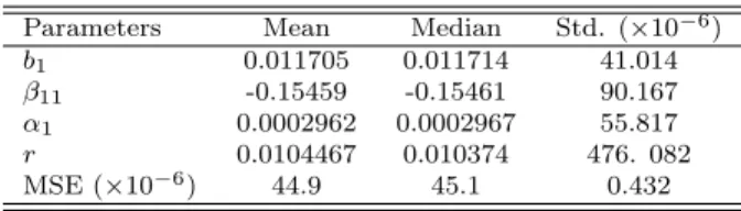
Table 1: Nonlinear least squares Estimation of Default-free Parameters

Parameters Mean Median Std. (×10−6₎

b1 0.011705 0.011714 41.014

β11 -0.15459 -0.15461 90.167

α1 0.0002962 0.0002967 55.817

r 0.0104467 0.010374 476. 082

MSE (×10−6_{) 44.9 45.1 0.432}

Table 2: Nonlinear least squares Estimation of Defaultable Parameters

Model θ b2 α2 β22 β21 ` PS 0.75 - - -1.5871 - 0.1634 RF - 0.0103 0.0805 -0.1623 1.9617 -MX 0.75 2.235e-006 - -2.2489 - 0.00178 Model λ1 λ2 c γ1 γ2 MSE PS 5.6902 0.60583 - - - 0.0115 RF - - 9.017e-005 0.2637 0.0077 0.0126 MX 2.3089 1.1843 - 0.11993 0.00181 0.00525

6.2.2 Estimation of Credit Indices

The estimates for the typical credit indices (Y2

Aaa, YAa2 , YA2, YBaa2 ) (standard error

in parentheses) assigned to each class (Aaa, Aa, A, Baa) for each model (PS, RF, MX) are shown in Table 3. For each model we haveY2

Aaa< YAa2 < YA2< YBaa2

as expected.

Table 3: Estimates of Credit Indices

Models Y2

Aaa YAa2 YA2 YBaa2

PS 3.5185(0.8461) 4.2031 (1.0879) 5.3475 (1.3829) 7.4638 (1.4285) RF -0.0169 (0.0738) 0.0937 (0.1090) 0.4277 (0.1265) 1.0233 (0.1787) MX 0.0806 (0.0184) 0.1641 (0.0265) 0.2922 (0.0350) 0.5462 (0.0465)

It speaks for the quality of a model if the values for Y2 _{do not vary too}

much for firms within one rating class. In view of the affine yield spread curve (22), this is equivalent to saying that theY2_{-sensitive part,−}1

Tψ˜2co(T,0), has an

appropriate shape. It is therefore an interesting test to solve for the credit index Y2_{of every individual firm, after having fixed all the remaining parameters given}

by the preceding estimation.

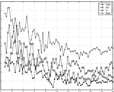
For the PS case, there exist a significant downward drift of the Y2_-value

from short-term bonds to long-term bonds as shown in Figure 1. This means that T 7→ −1

Tψ˜2co(T,0) is too steep, resulting in an overestimate of long term

yield spread at zero maturity (see (23)) also contributes to this phenomenon, see also [14].

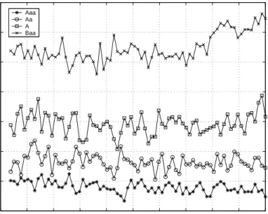
For the RF model notice that quite a few Aaa-rated bonds imply negative Y2_{-values (shown in Figure 2), which is not allowed in our affine setup. This}

means that the fixed yield spread part (the first two summands in (22)) is too large and has to be compensated by subtracting theY2_{-sensitive part.}

The MX model clearly outperforms PS and RF in this regard, as shown in Figure 3.

6.2.3 Spread Curves and Default Probabilities

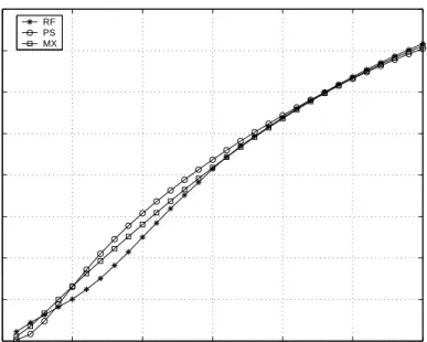
Figure 4 compares the yield spread curves for the Baa-rated class for the three different models. We can nicely see that the PS model has a zero yield spread at zero maturity, and how the MX model lies between the two extreme cases PS and RF.

We finally assume that the change from real-world measurePto risk-neutral measure ˜Pis given according to Section 5 by ˜b1=b1and ˜β1−β1= 0.02 (larger

mean reversion rate under P: |β˜1| <|β1|). This estimate of the market price

of risk is taken from [7]. Figure 5 shows the resulting default distributions for each model for rating class Baa. The main difference between the models is in the short end, where the PS model has a flat distribution function.

A

Proof of Lemma 4.1

We first prove an auxiliary result.

Lemma A.1. Y1

− is continuous on [0, T∆] a.s. Hence YT1∆− = limt↑↑T∆Yt1

exists a.s.

Proof. In view of (3), Ntg∧τ is a continuous local martingale for every stopping

timeτ < T∆andg∈Cb2(R+), where

N_tg:=g(Y1

t)−g(Y01)−

Z t

0

A1g(Ys1)ds (26)

(recall Remark 2.1 and (16)).

We now claim that there exists a universal constantC0=C0(t) such that

E[ sup

s<t∧T∆

(Y1

s)2]≤C0(1 + (Y01)2)eC0t. (27)

Indeed, in view of (11) and (26) Zn t :=Yt1∧Tn−Y 1 0 − Z t∧Tn 0 (b1+β1Ys1)ds

is a continuous local martingale with quadratic variation

hZn_i t=

Z t∧Tn 0

for everyn≥1. From Doob’s maximal inequality we obtain E[sup s≤t (Zn s)2]≤4E[(Ztn)2] = 4E[hZnit] = 4E "Z t∧Tn 0 α1Ys1ds # . Moreover, (Yt1∧Tn) 2₌ Ã Y01+ Z _t∧Tn 0 (b1+β1Ys1)ds+Ztn !2 ≤3 Ã (Y01)2+t Z _t∧Tn 0 (b1+β1Ys1)2ds+ (Ztn)2 ! . Combining this we get

gn(t) :=E[sup s≤t(Y 1 s∧Tn) 2_] ≤C1 Ã (Y01)2+E "Z _t∧Tn 0 ¡ (b1+β1Ys1)2+α1Ys1 ¢ ds #! , which implies gn(t)≤C2 µ 1 + (Y1 0)2+ Z t 0 gn(s)ds ¶ ,

where the constants C1, C2 depend only on t, α1, b1 and β1. Gronwall’s

in-equality yields

gn(t)≤C0(1 + (Y01)2)eC0t

withC0=C0(t, C2). Monotone convergence forn→ ∞yields (27).

On the other hand, we have by the same arguments as above that sup s≤t (Y1 s∧Tn−Y 1 s∧Tm) 2_≤2 Ã t Z t∧Tn t∧Tm (b1+β1Yu1)2du+ sup s≤t (Zn s −Zsm)2 ! and hence E · sup s≤t(Y 1 s∧Tn−Y 1 s∧Tm) 2 ¸ ≤2E " t Z t∧Tn t∧Tm (b1+β1Yu1)2du+ Z t∧Tn t∧Tm α1Ys1ds # ≤C3E ·µ 1 + sup s<t∧T∆ (Y1 s)2 ¶ (t∧Tn−t∧Tm) ¸

for alln ≥m, where C3 does not depend onm, n. Using (27) and dominated

convergence we conclude that lim m,n→∞E · sup s≤t(Y 1 s∧Tn−Y 1 s∧Tm) 2 ¸ = 0. Hence Y1 t∧Tn =Y 1

t∧Tn− converges uniformly int on compacts in probability to

Y1

Proof of Lemma 4.1 Recall that the stochastic basis is rich enough to carry an (Ft)-Brownian motionW. Define the (FT∆+t)t≥0-Brownian motion

W∆

t :=WT∆+t−WT∆, t≥0

and consider the stochastic differential equation dRt= (b1+β1Rt)dt+

p

2α1RtdWt∆

R0=YT1∆−.

(28) It is well known that a unique continuous (FT∆+t)t≥0-adapted strong solution

Rexists. Notice that

{(t−T∆)+≤c}={T∆≥t} ∪({T∆< t} ∩ {T∆≥t−c})∈ Ft ∀c≥0,

henceR(t−T∆)1{t≥T∆} is (Ft)-adapted.

We then define the continuous adapted process rt:=Yt11{t<T∆}+Rt−T∆1{t≥T∆}.

Letg ∈C2

c(R+). By Itˆo’s formula and since

R_T∆+t T∆ φudWu = R_t 0φT∆+udW ∆ u we have g(rt)−g(rt∧T∆) =g(R(t−T∆)+)−g(R0) = Z _(t−T∆)+ 0 A1g(Rs)ds+ Z _(t−T∆)+ 0 p 2α1Rsg0(Rs)dWs∆ = Z _t t∧T∆ A1g(rs)ds+ Z _t t∧T∆ √ 2α1rsg0(rs)dWs. Hence Ntg=g(rt)−g(r0)− Z _t 0 A1g(rs)ds = Z _t t∧T∆ √ 2α1rsg0(rs)dWs +g(rt∧T∆)−g(rt∧Tn)− Z t∧T∆ t∧Tn A1g(rs)ds +g(Y1 t∧Tn)−g(Y 1 0)− Z t∧Tn 0 A1g(Ys1)ds

satisfies fors≤t E[N_tg | Fs] = Z s s∧T∆ √ 2α1rug0(ru)dWu +E " g(rt∧T∆)−g(rt∧Tn)− Z t∧T∆ t∧Tn A1g(ru)du| Fs # +g(Ys1∧Tn)−g(Y 1 0)− Z _s∧Tn 0 A1g(Yu1)du =Nsg− Ã g(rs∧T∆)−g(rs∧Tn)− Z _s∧T∆ s∧Tn A1g(ru)du ! +E " g(rt∧T∆)−g(rt∧Tn)− Z _t∧T∆ t∧Tn A1g(ru)du| Fs # . This holds for any n ≥ 1. Letting n → ∞ we get by continuity of r and dominated convergence that

E[Ntg | Fs] =Nsg a.s.

HenceNg _{is a martingale and the proof of Lemma 4.1 is complete.}

References

[1] T. R. Bielecki and M. Rutkowski, Credit risk: modelling, valuation and hedging, Springer Finance, Springer-Verlag, Berlin, 2002.

[2] T. Bj¨ork, Arbitrage theory in continuous time, Oxford University Press, 1998.

[3] L. Chen and D. Filipovi´c,Pricing credit default swaps with default correla-tion and counterparty risk, Working paper, Princeton University, 2003. [4] P. Cheridito and D. Filipovi´c, Equivalent measure changes for

jump-diffusion processes, Working paper, Princeton University, 2003.

[5] J. Cox, J. Ingersoll, and S. Ross,A theory of the term structure of interest rates, Econometrica 53(1985), 385–408.

[6] R. Douady and M. Jeanblanc, A rating-based model for credit derivatives, Working Paper, Evry University, 2002.

[7] J. C. Duan and J. G. Simonato,Estimating and testing exponential-affine term structure models by kalman filter, Review of Quantitative Finance and Accounting13 (1999), 111–135.

[8] G. R. Duffee,Estimating the price of default risk, The Review of Financial Studies 12(1999), 41–59.

[9] D. Duffie, D. Filipovi´c, and W. Schachermayer, Affine processes and ap-plications in finance, forthcoming in The Annals of Applied Probability, 2002.

[10] D. Duffie and D. Lando,Term structure of credit spreads with incomplete accounting information, Econometrica 69(2001), 633–664.

[11] D. Duffie and K. Singleton,Modeling term structures of defaultable bonds, Rev. Finan. Stud.12(1999), 687–720.

[12] , Credit risk: Pricing, measurement, and management, Princeton University Press, 2003.

[13] S. N. Ethier and T. G. Kurtz,Markov processes, John Wiley & Sons Inc., New York, 1986, Characterization and convergence.

[14] K. Giesecke,Credit risk modeling and valuation: An introduction, Working Paper, Cornell University, 2003.

[15] J. Jacod and A. N. Shiryaev, Limit theorems for stochastic processes, Grundlehren der mathematischen Wissenschaften, vol. 288, Springer-Verlag, Berlin-Heidelberg-New York, 1987.

[16] R. A. Jarrow, D. Lando, and S. M. Turnbull,A markov model for the term structure of credit risk spreads, Rev. Finan. Stud.10(1997).

[17] R. A. Jarrow and S. M. Turnbull,Pricing derivatives on financial securities subject to credit risk, J. Finance50(1995).

[18] D. Lando, On Cox processes and credit-risky securities, Rev. Derivatives Res.2(1998), 99–120.

[19] K. Levenberg,A method for the solution of certain non-linear problems in least squares, Quart. Appl. Math.2(1944), 164–168.

[20] D. Marquardt,An algorithm for least squares estimation of nonlinear pa-rameters, SIAM J. Appl. Math.11(1963).

[21] D. Revuz and M. Yor, Continuous martingales and Brownian motion, Grundlehren der mathematischen Wissenschaften, vol. 293, Springer-Verlag, Berlin-Heidelberg-New York, 1994.

[22] L. C. G. Rogers and D. Williams,Diffusions, Markov processes, and mar-tingales. Vol. 2, Cambridge Mathematical Library, Cambridge University Press, Cambridge, 2000, Itˆo calculus, Reprint of the second (1994) edition.

Figure 1: Credit Indices for the PS Model 0 2 4 6 8 10 12 14 16 18 20 2 3 4 5 6 7 8 9 10 11 12

Bond Maturity (years)

Credit Indices

Aaa Aa A Baa

Figure 2: Credit Indices for the RF Model

0 2 4 6 8 10 12 14 16 18 20 −0.4 −0.2 0 0.2 0.4 0.6 0.8 1 1.2 1.4

Bond Maturity (years)

Credit Indices

Aaa Aa A Baa

Figure 3: Credit Indices for the MX Model 0 2 4 6 8 10 12 14 16 18 20 0 0.1 0.2 0.3 0.4 0.5 0.6 0.7

Bond Maturity (years)

Credit Indices

Aaa Aa A Baa

Figure 4: Spread Curves for Baa-Rating Class

0 5 10 15 20 25 30 0 0.005 0.01 0.015 0.02 0.025 0.03 0.035

Bond Maturity (years)

Credit Spreads

RF PS MX

Figure 5: Default Distributions for Baa-Rating Class 0 5 10 15 20 25 30 0 0.1 0.2 0.3 0.4 0.5 0.6 0.7 0.8 Time t (years) Default Probability RF PS MX