NBER WORKING PAPER SERIES DOWNSIDE RISK Andrew Ang Joseph Chen Yuhang Xing Working Paper 11824 http://www.nber.org/papers/w11824
NATIONAL BUREAU OF ECONOMIC RESEARCH 1050 Massachusetts Avenue
Cambridge, MA 02138 December 2005
Portions of this manuscript previously circulated in an earlier paper titled ”Downside Correlation and Expected Stock Returns.” The authors thank Brad Barber, Geert Bekaert, Alon Brav, John Cochrane, Randy Cohen, Qiang Dai, Kent Daniel, Bob Dittmar, Rob Engle, Wayne Ferson, Eric Ghysels, John Heaton, David Hirschleifer, N. Jegadeesh, Gautam Kaul, Jonathan Lewellen, Qing Li, Terence Lim, Toby Moskowitz,Lubos Pastor, Adam Reed, Akhtar Siddique, Rob Stambaugh, and Zhenyu Wang. We especially thank Cam Harvey (the editor) and Bob Hodrick for detailed comments. We also thank two anonymous referees whose comments greatly improved the paper. We thank seminar participants at Columbia University, Koc University, London Business School, LSE, Morgan Stanley, NYU, PanAgora Asset Management, UNC, USC, the American Finance Association, the Canadian Investment Review Risk Management Conference, the Conference on Financial Market Risk Premiums at the Federal Reserve Board, the European Finance Association, the Five Star Conference, an Inquire Europe meeting, a LA Society of Financial Analysts meeting, an NBER Asset Pricing meeting, a Q-Group meeting, the Texas Finance Festival, the Valuation in Financial Markets Conference at UC Davis, and the Western Finance Association for helpful discussions. The authors acknowledge funding from a Q-Group research grant. The views expressed herein are those of the author(s) and do not necessarily reflect the views of the National Bureau of Economic Research. ©2005 by Andrew Ang, Joseph Chen, and Yuhang Xing. All rights reserved. Short sections of text, not to exceed two paragraphs, may be quoted without explicit permission provided that full credit, including
Downside Risk
Andrew Ang, Joseph Chen, and Yuhang Xing NBER Working Paper No. 11824
December 2005
JEL No. C12, C15, C32, G12
ABSTRACT
Economists have long recognized that investors care differently about downside losses versus upside gains. Agents who place greater weight on downside risk demand additional compensation for holding stocks with high sensitivities to downside market movements. We show that the cross-section of stock returns reflects a premium for downside risk. Specifically, stocks that covary strongly with the market when the market declines have high average returns. We estimate that the downside risk premium is approximately 6% per annum. The reward for bearing downside risk is not simply compensation for regular market beta, nor is it explained by coskewness or liquidity risk, or size, book-to-market, and momentum characteristics.
Andrew Ang
Columbia Business School 3022 Broadway 805 Uris New York NY 10027 and NBER
[email protected] Joseph Chen
Marshall School of Business at USC Hoffman Hall 701
Los Angeles, CA 90089-1427 [email protected] Yuhang Xing
Jones School of Management Rice University
Room 230, MS 531 6100 Main Street Houston, TX 77004 [email protected]
1
Introduction
If an asset tends to move downward in a declining market more than it moves upward in a rising market, it is an unattractive asset to hold because it tends to have very low payoffs precisely when the wealth of investors is low. Investors who are sensitive to downside losses, relative to upside gains, require a premium for holding assets that covary strongly with the market when the market declines. Hence, in an economy with agents placing greater emphasis on downside risk than upside gains, assets with high sensitivities to downside market movements have high average returns. In this article, we show that the cross-section of stock returns reflects a premium for bearing downside risk.
As early as Roy (1952), economists have recognized that investors care differently about downside losses than they care about upside gains. Markowitz (1959) advocates using semi-variance as a measure of risk, rather than semi-variance, because semi-semi-variance measures downside losses rather than upside gains. More recently, the behavioral framework of Kahneman and Tversky’s (1979) loss aversion preferences, and the axiomatic approach taken by Gul’s (1991) disappointment aversion preferences, allow agents to place greater weights on losses relative to gains in their utility functions. Hence in equilibrium, agents who are averse to downside losses demand greater compensation, in the form of higher expected returns, for holding stocks with high downside risk.
According to the Capital Asset Pricing Model (CAPM), a stock’s expected excess return is proportional to its market beta, which is constant across periods of high and low market returns. As Bawa and Lindenberg (1977) suggest, a natural extension of the CAPM that takes into account the asymmetric treatment of risk is to specify asymmetric downside and upside betas. We compute downside (upside) betas over periods when the excess market return is below (above) its mean. We show that stocks with high downside betas have, on average, high unconditional average returns. We also find that stocks with high covariation conditional on upside movements of the market tend to trade at a discount, but the premium for downside risk dominates in the cross-section of stock returns.
Despite the intuitive appeal of downside risk, which closely corresponds to how individual investors actually perceive risk, there has been little empirical research into how downside risk is priced in the cross-section of stock returns. Early researchers found little evidence of a downside risk premium because they did not focus on measuring the downside risk premium using all individual stocks in the cross section. For example, Jahankhani (1976) fails to find any improvement over the traditional CAPM by using downside betas, but his investigation uses portfolios formed from regular CAPM betas. Similarly, Harlow and Rao (1989) only evaluate
downside risk relative to the CAPM in a maximum likelihood framework and test whether the return on the zero-beta asset is the same across all assets. All of these early authors do not directly estimate a downside risk premium by demonstrating that assets which covary more when the market declines have higher average returns.1
Our strategy for finding a premium for bearing downside risk in the cross section is as follows. First, we directly show at the individual stock level that stocks with higher downside betas contemporaneously have higher average returns. Second, we claim that downside beta is a risk attribute because stocks that have high covariation with the market when the market declines exhibit high average returns over the same period. This contemporaneous relationship between factor loadings and risk premia is the foundation of a cross-sectional risk-return relationship, and has been exploited from the earliest tests of the CAPM (see, among others, Black, Jensen and Scholes, 1972; Gibbons, 1982). More recently, Fama and French (1992) also seek, but fail to find, a relationship between post-formation market betas from an unconditional CAPM and realized average stock returns over the same period. Our study differs from these earlier tests by examining a series of short one-year samples using daily data, rather than a single long sample using monthly data. This strategy provides with greater statistical power in an environment where betas may be time-varying (see comments by Ang and Chen, 2004; Lewellen and Nagel, 2004).
Third, we differentiate the reward for holding high downside risk stocks from other known cross-sectional effects. In particular, Rubinstein (1973), Friend and Westerfield (1980), Kraus and Litzenberger (1976, 1983), and Harvey and Siddique (2000a) show that agents dislike stocks with negative coskewness, so that stocks with low coskewness tend to have high average returns. Downside risk is different from coskewness risk because downside beta explicitly conditions for market downside movements in a non-linear fashion, whereras the coskewness statistic does not explicitly emphasize asymmetries across down and up markets, even in settings where coskewness may vary over time (as in Harvey and Siddique, 1999). Since coskewness captures some aspects of downside covariation, we are especially careful to control for coskewness risk in assessing the premium for downside beta. We also control
1Pettengill, Sundaram and Mathur (1995) and Isakov (1999) estimate the CAPM by splitting the full sample into two subsamples that consist of observations where the realized excess market return is positive or negative. Naturally, they estimate a positive (negative) market premium for the subsample with positive (negative) excess market returns. In contrast, our approach examines premiums for asymmetries in the factor loadings, rather than estimating factor models on different subsamples. Price, Price and Nantell (1982) demonstrate that skewness in U.S. equity returns causes downside betas to be different from unconditional betas, but do not relate downside betas to average stock returns.
for the standard list of known cross-sectional effects, including size and book-to-market factor loadings and characteristics (Fama and French, 1993; Daniel and Titman, 1997), liquidity risk factor loadings (P´astor and Stambaugh, 2003), and past return characteristics (Jegadeesh and Titman, 1993). Controlling for these and other cross-sectional effects, we estimate that the cross-sectional premium is approximately 6% per annum.
Finally, we check if past downside betas predict future expected returns. We find that, for the majority of the cross-section, high past downside beta predicts high future returns over the next month, similar to the contemporaneous relationship between realized downside beta and realized average returns. However, this relation breaks down among stocks with very high volatility. We attribute this to two effects. First, the future downside covariation of very volatile stocks is difficult to predict using past downside betas – the average one-year autocorrelation of one-year downside betas for very volatile stocks is only 17.3% compared to 43.5% for a typical stock. This is not surprising because high volatility increases measurement error. Second, stocks with very high volatilities exhibit anomalously low returns (see Ang, Hodrick, Xing and Zhang, 2005). Fortunately, the proportion of the market where past downside beta fails to predict future returns is small (less than 4% in terms of market capitalization). Confirming Harvey and Siddique (2000a), we find that past coskewness predicts future returns, but the predictive power of past coskewness is not because past coskewness captures future exposure to downside risk. Hence, past downside beta and past coskewness are different risk loadings.
The rest of this paper is organized as follows. In Section 2, we present a simple model to show how a downside risk premium may arise in a cross-sectional equilibrium. The framework uses a representative agent with the kinked disappointment aversion utility function of Gul (1991) which places larger weight on downside outcomes. Section 3 demonstrates that stocks with high downside betas have high average returns over the same period that they strongly covary with declining market returns. In Section 4, we examine the predictive ability of past downside risk loadings. Section 5 concludes.
2
A Simple Model of Downside Risk
In this section, we show how downside risk may be priced cross-sectionally in an equilibrium setting. Specifically, we work with a rational disappointment aversion (DA) utility function that embeds downside risk following Gul (1991). Our goal is to provide a simple motivating example of how a representative agent with a larger aversion to losses, relative to his attraction
to gains, gives rise to cross-sectional prices that embed compensation for downside risk.2
We emphasize that our simple approach does not rule out other possible ways in which downside risk may be priced in the cross-section. For example, Shumway (1997) develops an equilibrium behavioral model based on loss averse investors. Barberis and Huang (2001) use a loss aversion utility function, combined with mental accounting, to construct a cross-sectional equilibrium. However, they do not relate expected stock returns to direct measures of downside risk. Aversion to downside risk also arises in models with constraints that bind only in one direction, for example, binding short-sales constraints (Chen, Hong and Stein, 2001; Hong and Stein 2003) or wealth constraints (Kyle and Xiong, 2001).
Rather than considering models with one-sided constraints or agents with behavioral biases, we treat asymmetries in risk in a rational representative agent framework that abstracts from additional interactions from one-sided constraints. The advantage of treating asymmetric risk in a rational framework is that the disappointment utility function is globally concave and provides solvable portfolio allocation problems, whereas optimal finite portfolio allocations for loss aversion utility may not exist (see Ang, Bekaert and Liu, 2005). Our example with disappointment utility differs from previous studies, because existing work with Gul’s (1991) first order risk aversion utility concentrates on the equilibrium pricing of downside risk for only the aggregate market, usually in a consumption setting (see, for example, Bekaert, Hodrick and Marshall, 1997; Epstein and Zin, 1990 and 2001; Routledge and Zin, 2003). While a full equilibrium analysis of downside risk would entail using consumption data, in our simple example and in our empirical work, we measure aggregate wealth by the market portfolio, similar to a CAPM setting.
Gul’s (1991) disappointment utility is implicitly defined by the following equation:
U(µW) = 1 K µZ µW −∞ U(W)dF(W) +A Z ∞ µW U(W)dF(W) ¶ , (1)
where U(W) is the felicity function over end-of-period wealth W, which we choose to be power utility, that is U(W) = W(1−γ)/(1−γ). The parameter 0 < A ≤ 1is the coefficient of disappointment aversion, F(·) is the cumulative distribution function for wealth,µW is the
certainty equivalent (the certain level of wealth that generates the same utility as the portfolio allocation determiningW) andK is a scalar given by:
K =P r(W ≤µW) +AP r(W > µW). (2) 2While standard power, or CRRA, utility also produces aversion to downside risk, the order of magnitude of a downside risk premium, relative to upside potential, is economically negligible because CRRA preferences are locally mean-variance.
Outcomes above (below) the certainty equivalentµW are termed “elating” (“disappointing”)
outcomes. If0< A <1, then the utility function (1) down-weights elating outcomes relative to disappointing outcomes. Put another way, the disappointment averse investor cares more about downside versus upside risk. If A = 1, disappointment utility reduces to the special case of standard CRRA utility, which is closely approximated by mean-variance utility.
To illustrate the effect of downside risk on the cross-section of stock returns, we work with two assets x and y. Asset x has three possible payoffs ux, mx and dx, and asset y has two
possible payoffs uy and dy. These payoffs are in excess of the risk-free payoff. Our set-up
has the minimum number of assets and states required to examine cross-sectional pricing (the expected returns ofx and y relative to each other and to the market portfolio, which consists ofxandy), and to incorporate higher moments (through the three states ofx). The full set of payoffs and states is given by:
Payoff Probability (ux, uy) p1 (mx, uy) p2 (dx, uy) p3 (ux, dy) p4 (mx, dy) p5 (dx, dy) p6.
The optimal portfolio weight for a DA investor is given by the solution to:
max
wx,wyU(µW), (3)
where the certainty equivalent is defined in equation (1),wx(wy) is the portfolio weight of asset
x(y), end of period wealthW is given by:
W =Rf +wxx+wyy, (4)
and Rf is the gross risk-free rate. An equilibrium is characterized by a set of asset payoffs,
corresponding probabilities, and a set of portfolio weights so that equation (3) is maximized and the representative agent holds the market portfolio (wx+wy = 1) with 0 < wx < 1 and
0< wy <1.
The equilibrium solution even for this simple case is computationally non-trivial because the solution to the asset allocation problem (3) entails simultaneously solving for both the certainty equivalent µW and for the portfolio weights wx and wy. In contrast, a standard portfolio
allocation problem for CRRA utility only requires solving the first order conditions for the optimalwxandwy. We extend a solution algorithm for the optimization (3) developed by Ang,
Bekaert and Liu (2005) to multiple assets. Appendix A describes our solution method and details the values used in the calibration. Computing the solution is challenging because for certain parameter values, equilibrium cannot exist because non-participation may be optimal for lowA under DA utility. This is unlike the asset allocation problem under standard CRRA utility, where agents always optimally hold risky assets that have strictly positive risk premia.
In this simple model, the regular beta with respect to the market portfolio (denoted byβ = cov(ri, rm)/var(rm)) is not a sufficient statistic to describe the risk-return relationship of an
individual stock. In our calibration, an asset’s expected returns increase withβ, butβ does not fully reflect all risk. This is because the representative agent cares in particular about downside risk, throughA <1. Hence, measures of downside risk have explanatory power for describing the cross-section of expected returns. One measure of downside risk introduced by Bawa and Lindenberg (1977) is the downside beta (denoted byβ−):
β− = cov(ri, rm|rm < µm)
var(rm|rm < µm)
, (5)
whereri (rm) is securityi’s (the market’s) excess return, andµm is the average market excess
return. We also compute a relative downside beta relative to the regular CAPM beta, which we denote byβ−−β.
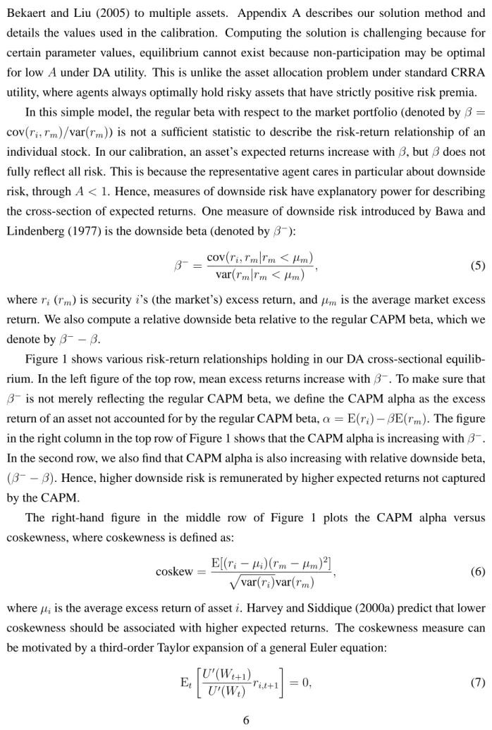
Figure 1 shows various risk-return relationships holding in our DA cross-sectional equilib-rium. In the left figure of the top row, mean excess returns increase withβ−. To make sure that
β− is not merely reflecting the regular CAPM beta, we define the CAPM alpha as the excess
return of an asset not accounted for by the regular CAPM beta,α = E(ri)−βE(rm). The figure
in the right column in the top row of Figure 1 shows that the CAPM alpha is increasing withβ−. In the second row, we also find that CAPM alpha is also increasing with relative downside beta,
(β−−β). Hence, higher downside risk is remunerated by higher expected returns not captured
by the CAPM.
The right-hand figure in the middle row of Figure 1 plots the CAPM alpha versus coskewness, where coskewness is defined as:
coskew= E[(ri−µi)(rm−µm)
2]
p
var(ri)var(rm)
, (6)
whereµiis the average excess return of asseti. Harvey and Siddique (2000a) predict that lower
coskewness should be associated with higher expected returns. The coskewness measure can be motivated by a third-order Taylor expansion of a general Euler equation:
Et · U0(W t+1) U0(W t) ri,t+1 ¸ = 0, (7)
whereW is the total wealth of the representative agent, andU0(·)can be approximated by: U0 = 1 +W U00r m+ 1 2W 2U000r2 m+· · · . (8)
The Taylor expansion in equation (8) is necessarily only an approximation. In particular, since the DA utility function is kinked, polynomial expansions of U, such as the expansions used by Bansal, Hsieh and Viswanathan (1993), may not be good global approximations if the kink is large (orAis very small).3 Nevertheless, measures like coskewness based on the Taylor approximation for the utility function should also have some explanatory power for returns.
Downside beta and coskewness may potentially capture different effects. Note that for DA utility, both downside beta and coskewness are approximations because the utility function does not have an explicit form (equation (1) implicitly defines DA utility). Since DA utility is kinked at an endogenous certainty equivalent, skewness, and other centered moments may not effectively capture aversion to risk across upside and downside movements in all situations. This is because they are based on unconditional approximations to a non-smooth function. In contrast, the downside beta in equation (5) conditions directly on a downside event that the market return is less than its unconditional mean. In Figure 1, our model shows that more negative coskewness is compensated by higher expected returns. However, the Appendix describes a case where CAPM alphas may increase as coskewness increases which is the opposite of the relation predicted by the Taylor expansion.
With DA utility, a representative agent is willing to hold stocks with high upside potential at a discount, all else being equal. A stock with high upside potential relative to downside risk tends to pay off more when an investor’s wealth is already high. Such stocks are not as desirable as stocks that pay off when the market decreases. Consider two stocks with the same downside beta, but with different payoffs in market up markets. The stock that covaries more with the market when the market rises has a larger payoff when the market return is high. This stock does not need as high an expected return in order for the representative agent to hold it. Thus, there is a discount for stocks with high upside potential. To measure upside risk, we compute an upside beta (denoted byβ+) that takes the same form as equation (5), except that we condition on movements of the market excess return above its average value:
β+ = cov(ri, rm|rm > µm)
var(rm|rm > µm)
. (9)
3Taylor expansions have been used to account for potential skewness and kurtosis preferences in asset allocation problems by Guidolin and Timmerman (2002), Jondeau and Rockinger (2003), and Harvey, Liechty, Liechty and M¨uller (2003).
Regular beta, downside and upside betas are, by construction, not independent of each other. To differentiate the effect of upside risk from downside risk, we introduce two additional measures. Similar to relative downside beta, we compute a relative upside beta (denoted by
β+ −β). We also directly examine the difference between upside beta and downside beta
by computing the difference between the two, (β+ −β−). In the last row of Figure 1, our model shows that controlling for regular beta or downside beta, higher upside potential is indeed remunerated by lower expected returns in our model.
Our simple example illustrates one possible mechanism by which compensation to downside risk may arise in equilibrium and how downside versus upside risk may priced differently. Of course, this example, having only two assets, is simplistic. Nevertheless, the model provides motivation to ask if downside and upside risk demand compensation in the cross section of US stocks, and if such compensation is different in nature from compensation for risk based on measures of higher moments, such as the Harvey-Siddique (2000a) coskewness measure. As our model shows, the compensation for downside risk is in addition to the reward already incurred in standard, unconditional risk exposures, such as the regular unconditional exposure to the market factor reflected in the CAPM beta. In our empirical work, we investigate a premium for downside risk also controlling for other known cross-sectional effects such as the size and book-to-market effects explored by Fama and French (1992, 1993), the liquidity effect of P´astor and Stambaugh (2003), and the momentum effect of Jegadeesh and Titman (1993).
3
Downside Risk and Realized Returns
In this section, we document that stocks that strongly covary with the market, conditional on down moves of the market, contemporaneously have high average returns. We document this phenomenon by first looking at patterns of realized returns for portfolios sorted on downside risk in Section 3.1. Throughout, we take care in controlling for the regular beta and emphasize the asymmetry in betas by focusing on relative downside beta in addition to downside beta. In Section 3.2, we examine the reward to downside risk controlling for other cross-sectional effects by using Fama-MacBeth (1973) regressions. We disentangle the different effects of coskewness risk and downside beta exposure in Section 3.3. Section 3.4 conducts various robustness tests. In Section 3.5, we show some additional usefulness of accounting for downside risk by examining if the commonly used Fama-French (1993) portfolios sorted by size and book-to-market characteristics exhibit exposure to downside risk.
3.1
Regular, Downside, and Upside Betas
Research DesignIf there is a cross-sectional relation between risk and return, then we should observe patterns between average realized returns and the factor loadings associated with exposure to risk. For example, the CAPM implies that stocks that covary strongly with the market have contemporaneously high average returns over the same period. In particular, the CAPM predicts an increasing relationship between realized average returns and realized factor loadings, or contemporaneous expected returns and market betas. More generally, a multi-factor model implies that we should observe patterns between average returns and sensitivities to different sources of risk over the same time period used to compute the average returns and the factor sensitivities.
Our research design follows Black, Jensen and Scholes (1972), Fama and MacBeth (1973), Fama and French (1992), Jagannathan and Wang (1996), and others, and focuses on the contemporaneous relation between realized factor loadings and realized average returns. More recently, in testing factor models, Lettau and Ludvigson (2001), Lewellen and Nagel (2004), and Bansal, Dittmar and Lundblad (2005), among others, all employ risk measures that are measured contemporaneously with returns. While both Black, Jensen and Scholes (1972) and Fama and French (1992) form portfolios based on pre-formation factor loadings, they continue to perform their asset pricing tests using post-ranking factor loadings, computed using the full sample. In particular, Fama and French (1992) first form 25 portfolios ranked on the basis of pre-formation size and market betas. Then, they compute ex-post factor loadings for these 25 portfolios over the full sample. At each month, they assign the post-formation beta of a stock in a Fama-MacBeth (1973) cross-sectional regression to be the ex-post market factor loading of the appropriate size and book-to-market sorted portfolio to which that stock belongs during that month. Hence, testing a factor relation entails demonstrating a contemporaneous relationship between realized covariance between a stock return and a factor with the realized average return of that stock.
Our work differs from Fama and MacBeth (1973) and Fama and French (1992) in one important way. Rather than forming portfolios based on pre-formation regression criteria and then examining post-formation factor loadings, we directly sort stocks on the realized factor loadings within a period and then compute realized average returns over the same period for these portfolios. Whereas pre-formation factor loadings reflect both actual variation in factor loadings as well as measurement error effects, post-formation factor dispersion occurs almost exclusively from the actual covariation of stock returns with risk factors. Moreover, we estimate
factor loadings using higher frequency data over shorter samples, rather than lower frequency data over longer samples. Hence, our approach has greater power.
A number of studies, including Fama and MacBeth (1973), Shanken (1992), Ferson and Harvey (1991), P´astor and Stambaugh (2003), among others, compute predictive betas formed using conditional information available at time t, and then examine returns over the next period. These studies implicitly assume that risk exposures are constant and not time-varying. Indeed, as noted by Daniel and Titman (1997), in settings where the covariance matrix is stable over time, pre-formation factor loadings are good instruments for the future expected (post-formation) factor loadings. If pre-formation betas are weak predictors of future betas, then using pre-formation betas as instruments will also have low power to detect ex-post covariation between factor loadings and realized returns. We examine the relation between pre-formation estimates of factor loadings with post-formation realized factor loadings in Section 4.
Empirical Results
We investigate patterns between realized average returns and realized betas. While many cross-sectional asset pricing studies use a horizon of one month, we work in intervals of twelve months, fromttot+12, following Kothari, Shanken and Sloan (1995). Our choice of an annual horizon is motivated by two concerns. First, we need a sufficiently large number of observations to condition on periods of down markets. One month of daily data provides too short a window for obtaining reliable estimates of downside variation. We check our the robustness of our results to using intervals of 24 months with weekly frequency data to compute downside betas. Second, Fama and French (1997), Ang and Chen (2004), and Lewellen and Nagel (2004) show that market risk exposures are time-varying. Very long time intervals may cause the estimates of conditional betas to be noisy. Fama and French (2005) also advocate estimating betas using an annual horizon using daily data.
Over every twelve months period, we compute the sample counterparts to various risk measures using daily data. We calculate a stock’s regular beta, downside beta as described in equation (5), and upside beta as described in equation (9). We also compute a stock’s relative downside beta, β−−β, a stock’s relative upside beta, β+−β, and the difference between upside beta and downside beta, β+−β−. Since these risk measures are calculated using realized returns, we refer to them as realizedβ, realizedβ−, realizedβ+, realized relative
β−, realized relativeβ+, and realizedβ+−β−.
In our empirical work, we concentrate on presenting the results of equal-weighted portfolios and equal-weighted Fama-MacBeth (1973) regressions. While a relationship between factor
sensitivities and returns should hold for both an average stock (equal-weighting) or an average dollar (value-weighting), we focus on computing equal-weighted portfolios because past work on examining non-linearities in the cross-section has found risk due to asymmetries to be bigger among smaller stocks. For example, the coskewness effect of Harvey and Siddique (2000a) is strongest for equal-weighted portfolios.4 We work with equally-weighted portfolios
to emphasize the differences between downside risk and coskewness. In a series of robustness checks, we also examine if our findings hold using weighted portfolios or in value-weighted Fama-MacBeth regressions. We concentrate only on NYSE stocks to minimize the illiquidity effects of small firms, but also consider all stocks on the NYSE, AMEX and NASDAQ in robustness tests.
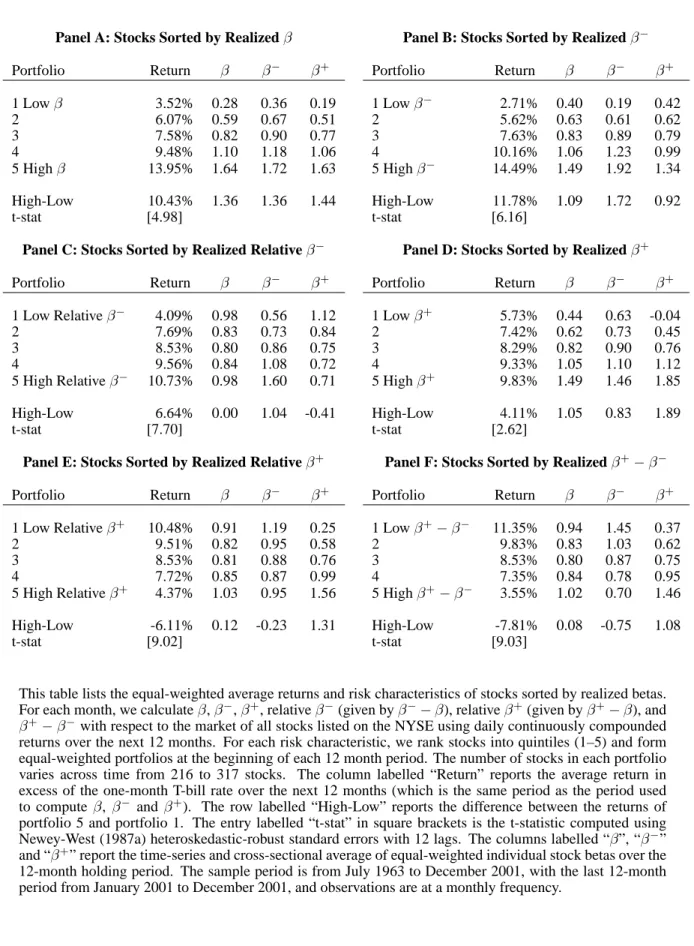
At the beginning of the one-year period at timet, we sort stocks into five quintiles based on their realizedβ, realizedβ−, realizedβ+, realized relativeβ−, realized relativeβ+, or realized
β+−β− over the next twelve months. In the column labelled “Return,” Table 1 reports the
average realized excess return from timettot+ 12in each equally-weighted quintile portfolio. The table also reports the average cross-sectional realizedβ,β−orβ+of each quintile portfolio. These average returns and betas are computed over the same 12-month period. Hence, Table 1 shows relationships between contemporaneous factor loadings and returns. Although we use a 1-year horizon, we evaluate 12-month returns at a monthly frequency. This use of overlapping information is more efficient, but induces moving average effects. To adjust for this, we report t-statistics of differences in average excess returns between quintile portfolio 5 (high betas) and quintile portfolio 1 (low betas) using 12 Newey-West (1987a) lags.5 The sample period is from July 1963 to December 2001, with our last 12-month return period starting in January 2001. As part of our robustness checks (below), we also examine non-overlapping sample periods.
Panel A of Table 1 shows a monotonically increasing pattern between realized average returns and realizedβ. Quintile 1 (5) has an average excess return of 3.5% (13.9%) per annum, and the spread in average excess returns between quintile portfolios 5 and 1 is 10.4% per annum, with a corresponding difference in contemporaneous market betas of 1.36. Our results are consistent with the earliest studies testing the CAPM, like Black, Jensen and Scholes (1972), who find a reward for holding higher beta stocks. However, this evidence per se does not mean that the CAPM holds, because the CAPM predicts that no other variable other than beta
4In their paper, Harvey and Siddique (2000a) state that they use value-weighted portfolios. From personal correspondence with Cam Harvey, the coskewness effects arise most strongly in equal-weighted portfolios rather than in value-weighted portfolios.
5The theoretical number of lags required to absorb all the moving average error effects is 11, but we include an additional lag for robustness.
should explain a firm’s expected return. Nevertheless, it demonstrates that bearing high market risk is rewarded with high average returns. Panel A also reports that the positive and negative components of beta (β− and β+). By construction, higher β− or higher β+ must also mean higher unconditional β, so high average returns are accompanied by highβ−, β+ and regular
β. Note that for these portfolios sorted by realized β, the spread in realizedβ−andβ+ is also similar to the spread in realizedβ. In the remainder of the panels in Table 1, we decompose the reward for unconditional market risk into downside and upside components.
Panel B shows that stocks with high contemporaneousβ−have high average returns. Stocks in the quintile with the lowest (highest)β−earn 2.7% (14.5%) per annum in excess of the risk-free rate. The average difference between quintile portfolio 5 and 1 is 11.8% per annum, which is statistically significant at the 1% level. These results are consistent with agents disliking downside risk and avoiding stocks that covary strongly when the market dips, such as the DA representative agent described in Section 2. Stocks with high β− must carry a premium in order to entice agents to hold them. An alternative explanation is that agents have no particular emphasis on downside risk versus upside potential. High β− stocks may earn high returns simply because, by construction, high β− stocks have high regularβ. The average β− spread between quintile portfolios 5 and 1 is very large (0.19 to 1.92), but sorting onβ−also produces variation in β and β+. However, the variation in β or β+ is not as disperse as the variation inβ−. Another possible explanation is that sorting on high contemporaneous covariance with the market mechanically produces high contemporaneous returns. However, this concern is not applicable to our downside risk measure since we are picking out precisely those observations for which stocks already have very low returns when the market declines. In Panels C and D, we demonstrate that it is the reward for downside risk alone that is behind the pattern of high
β−stocks earning high returns.
In Panel C of Table 1, we sort stocks by realized relative downside beta (β− − β). Relative downside beta focuses on the incremental impact of downside beta over the regular, unconditional market beta. Panel C shows that stocks with high realized relativeβ− have high average returns. The difference in average excess returns between portfolios 5 and 1 is 6.6% per annum and is highly significant with a robust t-statistic of 7.70. We can rule out that this pattern of returns is attributable to regular beta because theβ loadings are flat over the quintile portfolios. Hence, the high realized returns from high relativeβ−are produced by the exposure to downside risk, measured by highβ−loadings.
Panel D shows a smaller spread for average realized excess returns for stocks sorted on realized β+, relative to the spreads for β andβ− in Panels A and B. Sinceβ+ only measures exposure to a rising market, stocks that rise more when the market return increases should be
more attractive and, on average, earn low returns. We do not observe a discount for stocks that have attractive upside exposure. We find that low (high)β+stocks earn, on average, 5.7% (9.8%) per annum in excess of the risk-free rate. This pattern of high returns to highβ+loadings seems to be inconsistent with agents having strong preferences for upside potential, however, this measure does not control for the effects of regular β or for the effects ofβ−. Instead, the increasing pattern of returns in Panel D may be due to the patterns ofβ orβ−, which increase from quintile portfolios 1 to 5. The spread in regularβ is 1.05, while the spread inβ− is 0.83. From the CAPM, highβimplies high returns, and if agents dislike downside risk, highβ−also implies high returns. Hence, we now turn to measures that control for these effects to examine an upside risk premium.
In Panel E, we investigate the effect ofβ+ while controlling for regularβ by sorting stocks according to realized relative upside beta, (β+−β). Panel E shows that stocks with high realized relativeβ+have low returns. We find that high (low) relative β+ stocks earn, on average 4.4% (10.5%) per annum in excess of the risk-free rate. Furthermore, stocks sorted by relative upside beta produce a spread in β+ while keeping the spread in regularβ andβ− relatively flat. The differences in regular β and β− across the highest quintile and the lowest quintile (β+ −β) portfolios are relatively low at 0.12 and -0.23, respectively. In contrast, we obtain a wide spread in β+ of 1.31 between the highest quintile and the lowest quintile portfolios. This pattern of low returns to high relativeβ+stocks is consistent with agents accepting a discount for holding stocks with high upside potential, which would result from the DA agent equilibrium in Section 2.
Finally, we sort stocks by the realized difference between upside beta and downside beta
(β+ − β−) in Table 1, Panel F. We look at this measure to gauge the effect of upside risk
relative to downside risk. In Panel F, we observe a decreasing pattern in average realized excess returns with increasing(β+−β−). On average, we find that stocks with high (low)(β+−β−) earn 3.6% (11.4%) per annum in excess of the risk-free rate. While this direction is consistent with a premium for downside risk and a discount for upside potential, it is hard to separate the effects of downside risk independently from upside risk using these (β+−β−) portfolio sorts. The quintile portfolios sorted by (β+−β−)show little variation in regular β, but they show a decreasing pattern inβ−and an increasing pattern inβ+. Hence, it is difficult to separate whether the patterns in realized returns arise because of exposure to downside losses or exposure to upside gains. Thus, our preferred measures to examine downside or upside risk are relative
β−and relativeβ+in Panels C and E, which control for the effect ofβ.
In summary, Table 1 demonstrates that downside risk is rewarded in the cross-section of stock returns. Stocks with highβ−loadings earn high average returns over the same period that
are not mechanically driven by high regular, unconditional betas. Stocks that covary strongly with the market conditional on positive moves of the market command significant discounts. However, all these relations do not control for other known patterns in the cross-section of stock returns, which we now investigate.
3.2
Fama-MacBeth Regressions
A long literature from Banz (1981) onwards has shown that various firm characteristics also have explanatory power in the cross-section. The size effect (Banz, 1981), the book-to-market effect (Basu, 1983), the momentum effect (Jegadeesh and Titman, 1993), the volatility effect (Ang et al., 2005), exposure to coskewness risk (Harvey and Siddique, 2000a), exposure to cokurtosis risk (Scott and Horvarth, 1980; Dittmar, 2002), and exposure to aggregate liquidity risk (P´astor and Stambaugh, 2003), all imply different patterns for the cross-section of expected returns. We now demonstrate that downside risk is different from all of these effects by performing a series of cross-sectional Fama and MacBeth (1973) regressions at the firm level, over the sample period from July 1963 to December 2001.
We run Fama-MacBeth regressions of excess returns on firm characteristics and realized betas with respect to various sources of risk. We use a 12-month horizon for excess returns to correspond to the contemporaneous period over which our risk measures are calculated. Since the regressions are run using a 12-month horizon, but at the overlapping monthly frequency, we compute the standard errors of the coefficients by using 12 Newey-West (1987a) lags. Table 2 reports the results listed by various sets of independent variables in Regressions I-VI. We also report means and standard deviations to help gauge economic significance. We regress realized firm returns over a 12-month horizon (ttot+ 12) on realized market beta, downside beta and upside beta, (β,β−, andβ+) computed over the same period. Hence, these regressions capture a contemporaneous relationship between average returns and factor loadings or characteristics. We control for log-size, book-to-market ratio, and past 12-month excess returns of the firm at the beginning of the period t. We also include realized standard deviation of the firm excess returns, realized coskewness, and realized cokurtosis as control variables. All of these are also computed over the period from t tot + 12. We define cokurtosis in a similar manner to coskewness in equation (6): cokurt= E[(ri−µi)(rm−µm) 3] p var(ri)var(rm)3/2 , (10)
whereri is the firm excess return,rmis the market excess return,µiis the average excess stock
Stambaugh (2003) historical liquidity beta at timetto proxy for liquidity exposure.
In order to avoid putting too much weight on extreme observations, each month we Winsorize all independent variables at the 1% and 99% levels.6 Winsorization has been performed in cross-sectional regressions by Knez and Ready (1997), among others, and ensures that extreme outliers do not drive the results. It is particularly valuable for dealing with the book-to-market ratio, because extremely large book-to-market values are sometimes observed due to low prices, particularly before a firm delists.
We begin with Regression I in Table 2 to show the familiar, standard set of cross-sectional return patterns. While the regular market beta carries a positive coefficient, the one-factor CAPM is rejected because β is not a sufficient statistic to explain the cross-section of stock returns. The results of the regression confirm several CAPM anomalies found in the literature. For example, small stocks and stocks with high book-to-market ratios are linked with have high average returns (see Fama and French, 1992), while stocks with high past returns also continue to have high returns (see Jegadeesh and Titman, 1993). The very large and highly significant negative coefficient (-8.43) on the firm’s realized volatility of excess returns confirms the anomalous finding of Ang et al. (2005), who find that stocks with high return volatilities have low average returns. Consistent with Harvey and Siddique (2000a), stocks with high coskewness have low returns. Finally, stocks with positive cokurtosis tend to have high returns, consistent with Dittmar (2002).
In Regressions II-VI, we separately examine the downside and upside components of beta and show that downside risk is priced.7 We turn first to Regression II, which reveals that downside risk and upside risk are priced asymmetrically. The coefficient on downside risk is positive (0.069) and highly significant, confirming the portfolio sorts in Table 1. The coefficient onβ+is negative (-0.029), but lower in magnitude than the coefficient onβ−. These results are consistent with the positive premium on relativeβ−and the discount on relativeβ−reported in Panels C and E of Table 1.
Regression III shows that the reward for both downside and upside risk is robust to controlling for size, book-to-market and momentum effects. Note that asymmetric beta risk does not remove the book-to-market or momentum effects. But, importantly, the
Fama-6For example, if an observation for the firm’s book-to-market ratio is extremely large and above the 99th percentile of all the firms’ book-to-market ratios that month, we replace that firm’s book-to-market ratio with the book-to-market ratio corresponding to the 99th percentile. The same is done for firms whose book-to-market ratios lie below the 1%-tile of all firms’ book-to-market ratios that month.
7By construction,βis a weighted average ofβ−andβ+. If we place bothβandβ−on the RHS of Regressions
II-VI and omitβ+, the coefficients onβ−are the same to three decimal places as theβ−coefficients reported in Table 2. Similarly, if we specify bothβandβ+to be regressors, the coefficients onβ+are almost unchanged.
MacBeth coefficients for β− and β+ remain almost unchanged from their Regression II estimates at 0.064 and -0.025, respectively. While neither β− nor β+ are sufficient statistics to explain the cross-section of stock returns, Table 2 demonstrates a robust reward for holding stocks with high (low)β−(β+) loadings controlling for the standard size, book-to-market, and past return effects.
In Regressions IV-VI, accounting for additional measures of risk does not drive out the significance of β− but drives out the significance ofβ+. Once we account for coskewness risk in Regression IV, the coefficient on β+ becomes very small (0.003) and becomes statistically insignificant, with a t-statistic of 0.22. Controlling for coskewness also brings down the coefficient on β− from 0.064 in Regression III (without the coskewness risk control) to 0.028 in Regression IV (with the coskewness risk control). Nevertheless, the premium for downside risk remains positive and statistically significant. In Regression V, where we add controls for realized firm volatility and realized firm cokurtosis, the coefficient on downside risk remains consistently positive at 0.062, and also remains highly statistically significant, with a robust t-statistic of 6.00. While the preference function of Section 2 that weights downside outcomes more than upside outcomes implies a discount for upside risk, we observe these patterns in data only for Regressions II and III, where the upside discount is, in absolute value, about half the size of the premium for downside risk. After the additional controls beyond size, book-to-market, and momentum are included in Regressions IV and V, the discount for potential upside becomes fragile. Thus, the premium for downside risk dominates in the cross-section.
Finally, Regression VI investigates the reward for downside and upside risk controlling for the full list of firm characteristics and realized factor loadings. We lose five years of data in constructing the P´astor-Stambaugh historical liquidity betas, so this regression is run from January 1967 to December 2001. The coefficient on β− is 0.056, with a robust t-statistic of 5.25. In contrast, the coefficient on β+ is statistically insignificant, whereas the premium for coskewness is significantly negative, at -0.188. Since bothβ−and coskewness risk measure downside risk, and the coefficients on both risk measures are statistically significant, we carefully disentangle theβ−and coskewness effects in Section 3.4.
To help interpret the economic magnitudes of the risk premia reported in the Fama-MacBeth regressions, the last column of Table 2 reports the time-series average of the cross-sectional mean and standard deviation of each of the factor loadings or characteristics. The average market beta is less than one (0.83) because we are focusing on NYSE firms, which tend to be skewed towards large firms with relatively low betas. The average downside beta is 0.88, with a cross-sectional standard deviation of 0.74. This implies that for a downside risk premium of 6.9% per annum, a two standard deviation move across stocks in terms ofβ−corresponds to a
change in expected returns of2×0.069×0.74 = 10.2% per annum. While the premium on coskewness appears much larger in magnitude, at approximately -19% per annum, coskewness is not a beta and must be carefully interpreted. A two standard deviation movement across coskewness changes expected returns by2×0.188×0.19 = 7.1%per annum, which is slightly less than, but of the same order of magnitude as, the effect of downside risk.
The consistent message from the regressions in Table 2 is that reward for downside riskβ− is always positive at approximately 6% per annum and statistically significant. High downside beta is compensated for by high average returns, and this result is robust to controlling for other firm characteristics and risk characteristics, including upside beta. Moreover, downside beta risk remains significantly positive in the presence of coskewness risk controls. On the other hand, the reward for upside risk (β+) is not robust. A priori, we expect the coefficient onβ+ to be negative, but in data, it often flips sign and is insignificant when we control for other cross-sectional risk attributes. Thus, aversion to downside risk is priced more strongly, and more robustly, in the cross-section than investors’ attraction to upside potential.
3.3
Downside Beta Risk and Coskewness Risk
The Fama-MacBeth (1973) regressions in Table 2 demonstrate that both downside beta and coskewness have very robust, predictive power for the cross-section of stock returns. Since bothβ− and coskewness capture the effect of asymmetric higher moments and downside risk, we now measure the magnitude of the reward for exposure to downside beta, while explicitly controlling for the effect of coskewness. Table 3 presents the results of this exercise.
To control for the effect of coskewness, we first form quintile portfolios sorted on coskewness. Then, within each coskewness quintile, we sort stocks into five equally-weighted portfolios based onβ−. Both coskewness andβ−are computed over the same 12-month horizon for which we examine realized excess returns. After forming the 5× 5 coskewness and β− portfolios, we average the realized excess returns of eachβ−quintile over the five coskewness portfolios. This characteristic control procedure creates a set of quintileβ−portfolios with near-identical levels of coskewness risk. Thus, these quintileβ−portfolios control for differences in coskewness.
Panel A of Table 3 reports average excess returns of the 25 coskewness× β− portfolios. The column labelled “Average” reports the average 12-month excess returns of theβ−quintiles controlling for coskewness risk. The row labelled “High-Low” reports the differences in average returns between the first and fifth quintileβ− portfolios within each coskewness quintile. The last row reports the 5-1 quintile difference for the β− quintiles that control for the effect of
coskewness exposure. The average excess return of 7.6% per annum in the bottom right entry of Panel A is the difference in average returns between the fifth and firstβ−quintile portfolios that control for coskewness risk. This difference has a robust t-statistic of 4.16. Hence, coskewness risk cannot account for the reward for bearing downside beta risk.
In Panel A, the patterns within each coskewness quintile moving from low β− to high
β− stocks (reading down each column) are very interesting. As coskewness increases, the
differences in average excess returns due to differentβ−loadings decrease. The effect is quite pronounced. In the first coskewness quintile, the difference in average returns between the low and highβ−quintiles is 14.6% per annum. The average return difference in the low and highβ− portfolios decreases to 2.1% per annum for the quintile of stocks with the highest coskewness.
The reason for this pattern is as follows. As defined in equation (6), coskewness is effectively the covariance of a stock’s return with the square of the market return, or with the volatility of the market. A stock with negative coskewness tends to have low returns when market volatility is high. These are also usually, but not always, periods of low market returns. Volatility of the market treats upside and downside risk symmetrically, so both extreme upside and extreme downside movements of the market have the same volatility. Hence, the prices of stocks with large negative coskewness tend to decrease when the market falls, but the prices of these stocks may also decrease when the market rises. In contrast, downside beta concentrates only on the former effect by explicitly considering only the downside case. When coskewness is low, there is a wide spread inβ−because there is large scope for market volatility to represent both large negative and large positive changes. This explains the large spread in average returns across theβ−quintiles for stocks with low coskewness.
The small 2.1% per annum 5-1 spread for the β− quintiles for the highest coskewness stocks is due to the highest coskewness stocks exhibiting little asymmetry. The distribution of coskewness across stocks is skewed towards the negative side and is negative on average. Across the low to the high coskewness quintiles in Panel A, the average coskewness ranges from -0.41 to 0.09. Hence, the quintile of the highest coskewness stocks have little coskewness. This means that high coskewness stocks essentially do not change their behavior across periods where market returns are stable or volatile. Furthermore, the range ofβ− in the highest coskewness quintile is also smaller. The small range of β−for the highest coskewness stocks explains the low 2.1% spread for theβ−quintiles in the second last column of Panel A.
Panel B of Table 3 repeats the same exercise as Panel A, except we examine the reward for coskewness controlling for different levels ofβ−. Panel B first sorts stocks on coskewness before sorting on β−, and then averages across the β− quintiles. This exercise examines the coskewness premium controlling for downside exposure. Controlling forβ−, the 5-1 difference
in average returns for coskewness portfolios is -6.2%, which is highly statistically significant with a t-statistic of 8.17. Moreover, there are large and highly statistically significant spreads for coskewness in everyβ− quintile. Coskewness is able to maintain a high range within each
β−portfolio, unlike the diminishing range forβ−within each coskewness quintile in Panel A.
In summary, downside beta risk and coskewness risk are different. The high returns to high
β− stocks are robust to controlling for coskewness risk, and vice versa. Downside beta risk
is strongest for stocks with low coskewness. Coskewness does not differentiate between large market movements on the upside or the downside. For stocks with low coskewness, downside beta is better able to capture the downside risk premium associated only with market declines than an unconditional coskewness measure.
3.4
Robustness Checks
We now show that our results do not depend on the way we have measured asymmetries in betas or the design of our empirical tests. In particular, we show that our results are robust to measuring asymmetries with respect to different cutoff points across up-markets and down-markets. We also show that our results are robust to using longer frequency data. Finally, we show that our results are not driven by using equal weighting, concentrating on NYSE stocks, or using overlapping portfolios by checking robustness with respect to value weighting, including all stocks listed on NYSE, AMEX, and NASDAQ, and using non-overlapping portfolios.
We begin by using other cutoff points to determine up-markets and down-markets. Our measures ofβ−andβ+use returns relative to realized average market excess return. Naturally, realized average market returns vary across time and may have particularly low or high realizations. Alternatively, rather than using the average market excess return as the cutoff point between up-markets and down-markets, we can also use the risk-free rate or the zero rate of return as the cutoff point. We define downside and upside beta relative to the risk-free rate as: β− rf = cov(ri, rm|rm < rf) var(rm|rm < rf) and βrf+ = cov(ri, rm|rm > rf) var(rm|rm > rf) . (11)
We define downside and upside beta relative to the zero rate of return as:
β− 0 = cov(ri, rm|rm <0) var(rm|rm <0) and β0+ = cov(ri, rm|rm >0) var(rm|rm >0) . (12)
We show the correlations among these risk measures in Table 4, which reports the time-series averages of the cross-sectional correlations of regular beta and the various downside and upside risk measures. Table 4 shows thatβ−, βrf−, and β0− are all highly correlated with each other with correlations greater than 0.96. Similarly, we find thatβ+,βrf+, andβ0+are also highly
correlated with each other. Given these correlations, it is not surprising that reproducing Table 1 and Table 2 using either one of these alternative cutoff points yields almost identical results.8 Therefore, the finding of a downside risk premium is indeed being driven by emphasizing losses versus gains, rather than by using a particular cutoff point for the benchmark.
Table 4 also shows that the regular measure of beta is quite different from measures of downside beta and upside beta. The correlation between regular beta with downside beta or upside beta is 0.78 and 0.76, respectively. Therefore, downside beta and upside beta capture different aspects of risk, and are not simply reflective of the regular, unconditional market beta. Interestingly, the correlation between downside beta and upside beta is only around 0.46. Thus, a high downside risk exposures does not necessarily imply a high upside risk exposure. We examine further the cross-sectional determinants of future downside risk exposure below in Section 4.
We now turn to additional robustness checks to make sure our findings are being driven by variation in downside risk rather than by some statistical bias introduced by our testing method. In Table 5, we subject our results to a battery of additional robustness checks. Here, we check to see if our results are robust to excluding small stocks, using longer frequency data to compute β− and relativeβ−, creating value-weighted portfolios, using all stocks, and using non-overlapping annual observations.9 We report the robustness checks for realizedβ−
in Panel A and for realized relative β−in Panel B. In each panel, we report average 12-month (or 24-month) excess returns of quintile portfolios sorted by realizedβ−, or realized relativeβ−, over the same period. The table also reports the differences in average excess returns between quintile portfolios 5 and 1 with robust t-statistics.
One possible worry is that our use of daily returns introduces a bias due to non-synchronous trading. Indeed, one of the reasons for our focus on just the NYSE is to minimize these effects. To further check the influence of very small stocks, the first column of Table 5 excludes from our sample stocks that fall within the lowest size quintile. When small stocks are removed, the difference between quintile 5 and 1 for the stocks sorted by realized β− remains strongly statistically significant (with a robust t-statistic of 4.54) at 8.34% per annum, but is slightly reduced from the 5-1 difference of 11.8% per annum when small stocks are included in Table 1.
8These results are available upon request.
9In addition, we conduct further robustness checks that are available upon request. In particular, to control for the influence of non-synchronous trading, we also repeat our exercise using control for non-synchronous trading in a manner analogous to using a Scholes-Williams (1977) correction to compute the downside betas. Although this method is ad hoc, using this correction does not change our results. We also find that the point estimates of the premiums are almost unchanged when we exclude stocks that fall into the highest volatility quintile with the downside risk premium still statistically significant at the 1% level.
Similarly, the 5-1 difference in average returns for relativeβ− also remains highly significant. The second column computesβ−and (β−−β) using two years of weekly data, rather than one year of daily data. We compute weekly returns from Wednesdays to Tuesdays, and use two years of data to ensure that we have a sufficient number of observations to compute the factor loadings. We report the contemporaneous 24-month realized return over the same 24-month period used to measure the downside risk loadings. The table shows that there is no change in our basic message: there exists a reward for exposures to downside risk and relative downside risk.10
In the third column of Table 5, we examine the impact of constructing value-weighted portfolios rather than equal-weighted portfolios. Using value weighting preserves the large spreads in average excess returns for sorts byβ− and relativeβ−. In particular, the 5-1 spread of value-weighted quintile portfolios in realized returns from sorting on realizedβ−is 7.1% per annum. Although this has reduced from 11.8% per annum using equal-weighted portfolios in Table 1, the difference remains statistically significant at the 1% level. Similarly, the 5-1 spread in relative β− portfolios in Panel B reduces from 6.6% per annum using equal weighting to 4.0% per annum with value weighting. This difference is also significant at the 1% level.
In the fourth column, labelled “All Stocks,” we use all stocks listed on the NYSE, AMEX and NASDAQ, rather than restricting ourselves to stocks listed on the NYSE. We form equal-weighted quintile portfolios at the beginning of the period based on realized beta rankings. To keep our results comparable with our earlier results, we use breakpoints calculated over just the NYSE stocks. Using all stocks increases the average excess returns, so our main results using only the NYSE universe are conservative. The 5-1 spreads in average excess returns increase substantially using all stocks. For the β− (relative β−) quintile portfolios, the 5-1 difference increases to 15.2% (8.6%) per annum, compared to 11.8% (6.6%) per annum using only NYSE stocks. By limiting our universe to NYSE stocks, we deliberately understate our results to avoid confounding influences of illiquidity and non-synchronous trading.
In our last robustness check in Table 5, we use non-overlapping observations. While the use of the overlapping 12-month horizon in Tables 1 and 2 is statistically efficient, we examine the effect of using non-overlapping month periods in the last column of Table 5. Our 12-month periods start at the beginning of January and end in December of each calendar year. With non-overlapping samples, it is not necessary to control for the moving average errors with
10We have also reproduced the Fama-MacBeth regressions using risk measures calculated at the weekly frequency and found virtually identical results to Table 2. In addition, when we examine realized betas and realized returns over a 60-month horizon using monthly frequency returns, we find the same qualitative patterns that are statistically significant as using a 12-month horizon.
robust t-statistics, but we have fewer observations. Nevertheless, the results show that the point estimates of the 5-1 spreads are still statistically significant at the 1% level. Not surprisingly, the point estimates remain roughly unchanged from Table 1.
In unreported results, we also conduct additional robustness checks to value-weighting and using all stocks in a Fama-MacBeth regression setting. First, we run a set of value-weighted Fama-MacBeth regressions to make sure that small stocks are not driving our results. We do this by running a cross-sectional weighted least squares regression for each period, where the weights are the market capitalization of a firm at the beginning of each period. Using value-weighted regressions continues to produce a strong, statistically significant, positive relation between downside risk and contemporaneous returns with or without any additional controls. Similar to the results of using all stocks in the portfolio formations of Table 5, using all stocks in the Fama-MacBeth regressions only increases the magnitude of the downside risk premium, which remains overwhelmingly statistically significant.
3.5
Downside Risk in Size and Book-to-Market Portfolios
While we have demonstrated that exposures to high β− or high relative β− loadings are compensated by high average returns and this effect is consistent with investors placing greater weight on downside risk, we have not demonstrated that downside risk is useful in pricing portfolios sorted on other attributes. We now examine if portfolios of stocks sorted by other stock characteristics also exhibit contemporaneous exposure to downside risk. We focus on the Fama and French (1993) set of 25 portfolios sorted by size and book-to-market. To price these portfolios, Fama and French (1993) develop a linear asset pricing model that augments the excess market return factor,rm, with size and value factors (SMB and HML, respectively).
Table 6 examines if these portfolios exhibit exposure to downside risk, even after controlling for the standard Fama-French model.
In Table 6, we examine linear factor models of the form:
m=a+bm·rm+bm−·rm−+bSM B ·SMB+bHM L·HML, (13)
where rm− = min(rm, µm) equalsrm if the excess market return is below its sample mean, or
its sample mean otherwise. We estimate the coefficients bm, bm−, bSM B, andbHM L by GMM
using the moment conditions:
E(mr) = 0, (14)
of the test portfolios to downside risk.11 We conduct a χ2 specification test to examine the
fit with and fit without the downside risk exposure of various specifications of equation (13). Specifically, we compute a∆J χ2 difference test of Newey and West (1987b) using an optimal weighting matrix of the moment conditions under the unrestricted model of the alternative hypothesis. In particular, if we reject the null hypothesis thatb−m = 0, then we conclude that the restrictions imposed by the null hypothesis model that there is no downside risk exposure is too restrictive.
We consider two null models in Table 6, the null of the CAPM (Specification I) and the null of the Fama-French model (Specification III). In both alternatives (Specifications II and IV), Table 6 shows that the coefficient b−m is statistically significant at the 5% level. This indicates that for pricing the size and book-to-market portfolios, the downside portion of market return plays a significant role, even in the presence of the standard market factor. This is true even when we allow for SMB and HML to be present in the model. This is a strong result because the SMB and HML factors are constructed specifically to explain the size and value premia of the 25 Fama-French portfolios. For both the CAPM and the Fama-French model, the ∆J test strongly rejects both specifications in favor of allowing for downside market risk. For the Fama-French model, the p-value of the rejection is almost zero.
Thus, not only do individual stocks sorted directly onβ−loadings reveal a large reward for stocks with high downside risk exposure, but other portfolios commonly used in asset pricing also exhibit exposure to downside risk. In particular, linear factor model tests using the Fama and French (1993) size and book-to-market portfolios reject the hypothesis that these portfolios do not have exposure to downside market risk.
4
Predicting Future Downside Risk
The previous section demonstrates a strong positive relationship between stocks that exhibit high downside risk and returns for holding such stocks over the same period. While this is the essence of the relationship implied by a risk-to-reward explanation, knowing this relationship may not be of practical value if we cannot predict downside risk prior to the holding period. Therefore, we now examine if we can predict downside risk in a future period using past information. If today’s information can predict future downside risk, then we can form an
11Note that the factorr−
mis not traded, and thus the alpha of a time-series regression using the factors in equation
(13) does not represent the return of an investable strategy. Therefore, the alpha cannot be tested against the value of zero to examine possible mispricing. Similarly, we cannot compute a premium for a traded downside risk factor from equation (13).