Tasmanian School of Business and Economics
University of Tasmania
Discussion Paper Series N 2014
‐
04
Should ASEAN
‐
5 Monetary Policymakers Act Pre
‐
emp vely Against Stock Market Bubbles?
Mala RAGHAVAN
University of TasmaniaMardi DUNGEY
University of Tasmania, CAMA ANU
1 Should ASEAN-5 monetary policymakers act pre-emptively
against stock market bubbles?
Mala Raghavan a and Mardi Dungey b
a
Tasmanian School of Business and Economics, University of Tasmania, Locked Bag 1317, Launceston, TAS 7250, Australia
b
Tasmanian School of Business and Economics, University of Tasmania, GPO Box 84, Hobart, TAS 7001, Australia
Stock market rises and asset price inflation in ASEAN economies have raised the question of whether monetary authorities of these economies should act pre-emptively against these rising trends to prevent impending financial crises. Using a structural VECM which incorporate mixed data characteristics we examine the effects and interactions between monetary policy and stock market shocks for Singapore, Malaysia, Thailand, Indonesia and the Philippines. The results suggest that monetary policy focused on the stock market detracts from price stability objectives, in particular because containing a stock market bubble may inadvertently depress output and inflation.
JEL classification: C32, C53, E44, E52 , F33
Keywords: SVECM, monetary policy, stock market, ASEAN
2 I Introduction
Sustained rapid credit growth coupled with large increases in asset and stock prices is significantly associated with pre-crisis conditions in financial markets (Reinhart and Rogoff, 2009; White, 2009; Adrian and Shin, 2010; Mishkin, 2011; Allen and Rogoff, 2011). Cumulative output losses following a financial crisis and the cost of fiscal support programs
can be substantial (Bordo et al., 2001; Laeven and Valencia, 2012). Consequently, there is
support for monetary policy aimed at pre-emptively leaning against stock market misalignments; see Reinhart and Rogoff (2009), Mishkin (2011). The existing empirical evidence for the degree to which such policies may conflict with the more common price
stability goals of monetary policy is limited to OECD economies1, and evidence for emerging
economies is to our knowledge unexplored.
The successful transition of the emerging markets of Asia to full development is important both to the world economy, and as a model for other emerging markets. The Asian share of world GDP has risen to 34% by 2012 (19% excluding China), and with 60% (41%
excluding China) of world population these are important markets2. Monetary policy in these
emerging markets is significant not only to the economies of the respected countries, but also increasingly becoming important to the world economy.
This paper focuses on the interdependence of monetary policy and stock markets in the post-1997 Asian crisis period for the ASEAN-5 economies of Singapore, Malaysia, Thailand, Indonesia and the Philippines. In particular we are concerned to assess whether monetary policy in these economies can achieve both price stability and financial stability by identifying and leaning against stock price misalignments while operating in a small open economy environment.
1
See for example Kuttner (2011), Bjorland and Leitemo (2009), Katrin and Stefan (2008), Neri (2004), Cassola and Morana (2002), Cheung and Ng (1998).
2
Source:http://www.quandl.com/economics/gdp-as-share-of-world-gdp-at-ppp-all-countries and
3 The economic experience of the ASEAN-5 in the last 15 years provides an excellent testing ground for assessing the interaction of monetary policy shocks with the financial sector and subsequent effects on the real economy. ASEAN financial markets generally experience higher volatility than their OECD counterparts, and comparatively lower liquidity. During the float of the Thai bhat in July 1997, all of these markets experienced significant stock market falls, rapid withdrawal of funds by foreign investors and local currency depreciation. For Malaysia, Thailand, Indonesia and the Philippines substantial economic recession followed. The crisis was severe enough to significantly impact monetary policy mechanisms for many of these countries; Thailand moved from a fixed to floating exchange rate regime with inflation targeting, Malaysia reverted to a fixed exchange rate regime, Indonesia removed its managed float and adopted inflation targeting, and the Philippines removed its remaining few impediments to a freely floating exchange rate regime but retained its combined monetary growth/inflation targeting monetary policy stance, moving to inflation targeting in 2002. Singapore, the most developed and least affected of the ASEAN-5 markets, retained its managed currency throughout. In the 21st century the relatively high growth and high interest rate environments of these economies has again attracted capital inflow, excess liquidity, and a perceived higher risk of emerging price bubbles (Shimada and Yang, 2010; Hong and Tang, 2010).
Using a data and theory-consistent structural vector error correction model (SVECM) and developing economy applications, we consider the impact of shocks from stock markets and monetary policy, and their interaction on real economy outcomes. The recent
development in SVECM methodology allows us to incorporate both the mixed I(1) and I(0)
nature of the data and empirically supported cointegrating relationships within the same modelling framework in the manner suggested in Pagan and Pesaran (2008) and Fisher and
4
Huh (2012). This paper provides a first use of these tools to examine the role of equity
markets in the real economy.
We find evidence of a long run relationship between stock market prices and indicators of macroeconomic conditions such as real output, money stock and the exchange rate. The interactions of stock market shocks and monetary policy shocks in the model strongly suggest that monetary policy focussed on the stock market is likely to be incompatible with inflation targeting or price stability objectives in these economies, because while aiming to contain stock market bubbles they may inadvertently depress output and inflation. However, we also find that monetary policy itself may not be sufficient to control or avoid large stock market price fluctuations. This suggests that other policy instruments such as strengthening financial supervision and macro-prudential regulation polices should be sought along with monetary
policy to constrain any future price bubbles (Boivin et al., (2010); Mishkin, (2011); Gali
(2013).
The paper proceeds as follows. Section II reviews the theoretical and empirical evidence linking the stock markets and monetary policy. The modelling methodology and the identification implementation for this paper are described in Sections III and IV. The results are discussed in Section V, and Section VI concludes.
II Monetary Policy and the Stock Market
There are good reasons to anticipate that monetary policy and developments in the stock market may be interdependent. Stock prices provide forward looking information on the expected future path of the economy (Gordon, 1962; Vickers, 2000), and in the absence of better information may provide a suitable indicator of private sector expectations (Vickers, 2000). In a forward looking inflation targeting regime stock prices are likely to incorporate output and inflation expectations (Goodhart and Hofmann, 2000). However, stock prices may
5 also influence consumption, investment and credit availability - through the wealth channel, Tobin’s Q and the credit channel respectively. Higher stock prices may lead to a rise in consumption expenditure, investment levels and the value of collateral; thereby increasing demand. Thus, central banks which actively manage aggregate demand also have incentives to monitor stock prices as short-run indicators about the state of the economy. Unanticipated monetary policy changes may also influence stock prices, either directly due to changes in expected interest rates or due to changes in expected future dividends and stock returns. Contractionary monetary policy is expected to reduce stock prices while expansionary policy inflates them.
While positive expectations about future growth can increase demand for stocks, and increase their prices, asset price inflation can threaten the stability of the economy, particularly if it does not reflect fundamentals. Rising stock prices which are used as collateral for further lending can generate a bubble, which may become further inflated as lenders rely on appreciation to shield themselves from losses. The presence of such bubbles implies a potential role for central banks to contain them by leaning against `excessive’ increases in stock prices (Gali, 2013).
There is disagreement in the literature on the potential usefulness of monetary policy in containing stock price bubbles – see Mishkin (2011). On one hand is the argument that financial instability leads to costly adverse macroeconomic consequences supporting “pre-emptive tightening” to moderate price bubbles rather than “pre-“pre-emptive easing” to deal with
the aftermaths (Bean, 2010; White, 2009; Cechetti et al., 2000). However, given the
difficulties inherent in identifying bubbles, (see Gurkaynak, 2008; for an overview) and uncertainty about whether they can be influenced by monetary policy actions, others argue that monetary policy should serve exclusively as a counter-cyclical tool and stock price
6 fluctuations which do not affect inflation within the central bank’s forecast horizon should be ignored; Bernanke and Gertler (2001), Kohn (2006, 2009), Kuttner (2011).
Boivin et al. (2010), Mishkin (2011) and Gali (2013) argue that the case for monetary
policy to lean against any asset price bubble depends on the sources of the imbalances and the nature of other regulatory instruments available. If asset price bubbles are specific to a particular sector of the economy, and a well-targeted macroeconomic prudential tool is available, then monetary policy need only play a minor role. On the other hand, if asset price imbalances affect the entire economy, then monetary policy will be able to play a more substantial role in containing a bubble.
The empirical question as to whether monetary policy can effectively lean against stock market shocks requires a system incorporating stock prices, inflation, output, exchange rate and monetary policy variables without necessarily identifying bubble conditions. A number of existing papers have incorporated equity markets into more traditional Vector Autoregression (VAR) models; such as Lee (1992), Patelis (1997), Thorbecke (1997), Millard and Wells (2003) and Neri (2004), each of which use a traditional Cholesky decomposition to identify the shocks. However, stronger evidence of the monetary policy shocks on stock markets is found using alternative identifications such as using high frequency data from the futures market within the VAR framework in Bernanke and Kuttner (2005) and D’Amico and Farka (2011), long run neutrality in Lastrapes (1998) and Rapach (2001), or combinations of long and short run restrictions in Bjorland Leitemo (2009). In a VECM framework, stock markets were found to play an important role in Euro Area monetary transmission by Cassola and Morana (2002). Each of these studies, however, considered only evidence from developed economies.
This paper contributes to and extends the existing literature in two main areas. First, using recent development in SVECM methodology and developing economy application, it
7 analyses the interaction between monetary policy and stock prices of small emerging open economies of ASEAN. Two, the model framework identifies the long run relationship of real stock prices with domestic variables and it emphasises the transmission of domestic and foreign shocks to the domestic economy by allowing the stock prices to react to all variables contemporaneously. This reflects the forward looking nature of the stock prices in the model.
III Methodology
A SVECM framework incorporating both and variables in the system takes
direct advantage of potential cointegration relationships between some of the variables.
A SVECM with the intercept terms suppressed for ease of exposition can be written as:
(1)
Where is a difference operator, is a vector of variables, is a matrix of
long-run coefficients, the are matrix of short-run coefficients
with normalised across the main diagonal and is a multivariate white noise
error process with zero mean and a diagonal covariance matrix
Assuming that the matrix is invertible, equation 1 can be written as
(2)
Where and which relates the reduced form errors
to the underlying structural errors . The SVECM innovations are linked to the reduced
form innovations by
(3)
where are all matrices. Exact identification of requires the
imposition of additional restrictions on . A common approach in the
literature is to apply identification restrictions that are consistent with economic theory and stylised facts.
8
The existence of cointegration among I(1) variables in the model can provide extra
identifying restrictions as the integrated variables must be driven by one or more permanent
shock (Pagan and Pesaran, 2008). Since the in (2) can be written as where is a
matrix that contains the long run relationship and is a matrix of the "speed of adjustment"
coefficients for I(1) variables together with the aggregate effects for I(0) variables.
Substituting into equation 2 produces the model in error correction form:
(4)
In an -variable system, if variables are I(1) with cointegrating vectors, is
subject to permanent shocks, which are not cointegrated with other variables and
thus do not contribute to long run adjustments. The transitory shocks are of two types.
Firstly, shocks are from I(1) variables which perform the adjustment to the long rung
cointegrating relationships. Secondly shocks are from I(0) associated with
adjustment coefficient.3 Both and are matrices with rank . The columns of
corresponding to the I(0) variables contain all zeros except for a unit element relating to its
own lag while the dynamics of any I(0) variable is written in terms of differences and its
lagged level. A detailed explanation together with examples can be found in Fisher and Huh
(2012) and Dungey et al. (2013).
Using the Wold decomposition theorem, can be written as
(5)
where is a polynomial of order in the lag operator. Assuming that the first )
shocks are permanent and subsequent ) shocks are transitory can be
written as
(
) (6)
3 variables are not required to be transitory, they can be permanent shocks (see Fisher, Huh and Pagan,
2013). In our analysis, there are no permanent effects identified for the variables in any of the five economies.
9 An estimated SVECM model can then be used to analyse the dynamic responses of the domestic variables to various shocks by estimating the impulse response functions and historical decomposition.
IV Data and Empirical Specification
The data set contains monthly observations for eight variables over the sample period January 2000 to December 2011 for each of the ASEAN-5 economies to construct SVECM models with small open economy properties. The sample period covers the post-1997 East Asian financial crisis but includes the current global financial crisis (GFC).
Two foreign variables are included - world oil price inflation (oil), to account for inflation
expectations (see for example Sims (1992)) and the Federal funds rates (r*), commonly used
to proxy for world financial conditions (see for example Cushman and Zha, 1997; Kim and Roubini, 2000; Dungey and Pagan, 2000, 2009). In each country, six domestic variables are
selected: the log of industrial production index (y) and consumer price inflation (π) as the
target variables of monetary policy; short-term interest rates (r) are used as the monetary
policy instrument while the log of monetary aggregate (M1) represents the liquidity level in
the economy and the log of real exchange rate (q), as the information market variable that
captures the open nature of these economies and the importance of international trades and capital flows. These five domestic variables are also the standard set of variables used in the monetary literature to represent open economy monetary business cycle models (see for
example Sims, 1992). In addition, we included the log of real stock price index (s) in our
SVECM model as a proxy for the stock price channel. Detailed data descriptions and sources are provided in Table 1A, in Appendix A.
In summary, the model for each economy contains the following variables:
10 Fig. 1. Data for the ASEAN-5
Fig. 1 shows the data series for each of the ASEAN-5 economies. The GFC period is a notable feature in these figures. Prior to the crisis period, there was a relatively large rise in inflation, mainly due to an oil price shock. The inflationary pressure caused the central banks of these economies to embark on monetary tightening, as evidenced by the rise in domestic interest rates, which resulted in huge capital inflows, leading to excess liquidity. In late 2008 there was capital flight out of the region due to the crisis in developed markets, putting
3.5 4 4.5 5 5.5 Jan -0 0 Jan -0 1 Jan -0 2 Jan -0 3 Jan -0 4 Jan -0 5 Jan -0 6 Jan -0 7 Jan -0 8 Jan -0 9 Jan -1 0 Jan -1 1 Output -5 0 5 10 15 20 Jan -0 0 Jan -0 1 Jan -0 2 Jan -0 3 Jan -0 4 Jan -0 5 Jan -0 6 Jan -0 7 Jan -0 8 Jan -0 9 Jan -1 0 Jan -1 1 Inflation 0 5 10 15 20 Jan -0 0 Jan -0 1 Jan -0 2 Jan -0 3 Jan -0 4 Jan -0 5 Jan -0 6 Jan -0 7 Jan -0 8 Jan -0 9 Jan -1 0 Jan -1 1 Interest Rate 4 6 8 10 12 14 16 Jan -0 0 Jan -0 1 Jan -0 2 Jan -0 3 Jan -0 4 Jan -0 5 Jan -0 6 Jan -0 7 Jan -0 8 Jan -0 9 Jan -1 0 Jan -1 1 Monetary Aggregate M1 1 2 3 4 5 6 Jan -0 0 Jan -0 1 Jan -0 2 Jan -0 3 Jan -0 4 Jan -0 5 Jan -0 6 Jan -0 7 Jan -0 8 Jan -0 9 Jan -1 0 Jan -1 1
Real Exchange Rate
5 5.5 6 6.5 7 7.5 8 8.5 Jan -0 0 Jan -0 1 Jan -0 2 Jan -0 3 Jan -0 4 Jan -0 5 Jan -0 6 Jan -0 7 Jan -0 8 Jan -0 9 Jan -1 0 Jan -1 1
11 downward pressure on stock prices. Oil prices fell causing a fall in inflationary pressure, followed by an easing of monetary policy.
Each of the production index, monetary aggregates, real exchange rate, and real stock
prices are well supported as I(1) series while oil price inflation, Federal funds rate and
domestic inflation show evidence of being stationary in all economies. Augmented Dickey- Fuller unit root tests for all variables over the whole sample are reported in Table 2A in Appendix A. Although the unit root tests indicate that the interest rate series are non-stationary, interest rates are assumed to be stationary and highly persistent, in line with existing empirical literature (see Sack and Weiland, 2000; Dungey and Osborn 2013).
Cointegrating Relationships and Long Run Restrictions
Two cointegrating relationships are evident between the four I(1) series according to the
Johansen cointegration test (see Table 3A in Appendix A). The first of these is between the real stock prices, output and monetary aggregates for each economy – this suggests that equity investors are responsive to output and monetary conditions in the long run. This is consistent with existing evidence that future growth rates in real activity and money growth are positively related to real stock returns in industrialized economies; see for example Cheung and Ng (1998), Asprem (1989) and Mandelker and Tandon (1985). The second long run relationship is between output, real stock prices and the real exchange rate – which builds upon the open economy Mundell-Fleming model extended to include stock markets which
affect output through wealth and investment channels (Murudoglu et al., 2001; Cassola and
Morana, 2002). This is also consistent with Wongbangpo and Sharma (2002), who found long run relationship between ASEAN-5 stock markets and their macroeconomic variables.
To incorporate these relationships into the SVECM structure the stationary residuals from each relationship are extracted from the first stage Engle-Granger method for inclusion
12 in the model. The results are reported in Table 1, where at 5% significance level the residuals series were found to be stationary, thus indicating that the two long run relationships exists
between the four I(1) variables.
Table 1. Engle-Granger Two-step Cointegration Tests
t-stat on ecmt series
Singapore st = 5.969 + 1.289yt - 0.331M1t + ecm1,t yt = -3.597 + 1.344qt + 0.413st + ecm2,t -3.383 -4.131 Malaysia st = 1.344 + 0.579yt + 0.254M1t + ecm1,t yt = 0.480 + 0.368qt + 0.338st + ecm2,t -3.620 -3.116 Thailand st = 0.800 + 0.586yt + 0.403M1t + ecm1,t yt = 0.814 + 0.871qt + 0.299st + ecm2,t -2.553 -2.643 Indonesia st = -8.202 + 0.043yt + 1.082M1t + ecm1,t yt = 2.850 + 0.306qt + 0.0062st + ecm2,t -3.009 -4.602 Philippines st = 1.450 + 0.408yt + 0.339M1t + ecm1,t yt = 2.759 + 0.199qt + 0.215st + ecm2,t -2.728 -3.969
Notes: Two cointegrating vectors exist between the four I(1) variables. The first cointegrating relationship is between s, y and M1 and the second cointegrating relationship is between y, q and s. t-stat of each ecm series is calculated and tested if the series has unit root. The test critical value at 5% is -1.944
Since the SVECM model has n=8 variables with four I(1) variables, linked by two
cointegrating vectors, the system is subject to two permanent shocks. These permanent shocks are assumed to originate from output and monetary aggregates, representing productivity and income velocity of money shocks - thus the corresponding element of the matrix α is zero for these shocks. The real exchange rate and real stock price shocks are
13 assumed to be transitory and these variables undertake the adjustment required for the
cointegrating relationship to hold. For the given these
restrictions are shown in equation 8. As the oil price inflation, interest rates and inflation
series are I(0) variables, the lagged level of the dependent variables are included in the β
matrix to correct for the levels effect which would be lost in using a standard VECM (see Fisher and Huh, 2012).
13 23 24 13 16 27 28 41 42 43 45 45 51 52 55 56 61 72 73 74 75 76 81 82 83 84 85 86 0 0 Π 0 0 0 0 0 0 0 0 0 0 0 0 1 0 0 0 0 0 0 0 0 1 0 0 0 0 1 0 0 0 0 0 0 0 0 0 0 1 0 0 0 0 0 0 0 0 0 0 0 0 0 0 0 1 0 0 0 0 0 0 0 0 αβ' 0 β 0 α ' 1 0 (8)
Short Run Restrictions
The specification of the contemporaneous relationships and short-run dynamics are shown in equation 9. A number of restrictions are drawn from the existing literature. First, in line with the small open economy assumption, foreign block exogeneity restrictions are imposed, by assuming that neither contemporaneous nor lagged values of ASEAN-5 variables affect the oil price and Federal funds rate.
The contemporaneous matrix is initially based on conventional causal ordering
assumptions, and hence A0 is lower triangular. Oil prices are assumed exogenous to all other
variables in the model, and the Federal Funds rate is assumed to be affected only by oil. In the domestic components of the model, output is influenced by oil, but not the Federal Funds rate. The specification of the domestic inflation equation reflects a basic Phillips curve augmented by oil prices as a measure of inflationary expectations as in Sims (1992).
14 Contemporaneously, domestic inflation responds to oil and output shocks. Similar restrictions
are also imposed by Kim and Roubini (2000) for OECD economies and Raghavan et al
(2012) for the Malaysian economy. Since oil is a crucial input for most economic sectors, the price of oil is assumed to affect both the real sector and inflation contemporaneously. Further, we assume firms do not change their output and prices in response to unexpected changes in output, inflation, financial signals or monetary policy within a month due to inertia, adjustment costs and planning delays; however, the lag structure incorporates their reactions from the following month. The lag structure also contains the restriction that real interest rates are the appropriate measure of influence on output, which is achieved by setting a
in matrix Ai. i 11 0 i i 21 21 22 0 i 31 31 0 0 41 43 ' t t 0 0 53 54 0 0 0 63 64 65 0 0 0 0 0 0 71 72 73 74 75 76 0 0 0 0 0 0 0 81 82 83 84 85 86 87 1 0 0 0 0 0 0 0 a 0 0 0 0 0 0 0 a 1 0 0 0 0 0 0 a a 0 0 0 0 0 0 a 0 1 0 0 0 0 0 a 0 a 0 a 1 0 0 0 0 X X + 0 0 a a 1 0 0 0 0 0 a a a 1 0 0 a a a a a a 1 0 a a a a a a a 1 o t i i i i i i 33 35 35 36 37 38 i i i i i i 41 43 44 45 36 37 t i i i i i 53 54 55 57 i i i i i i 63 64 65 66 67 67 i i i i i i i i 71 72 73 74 75 76 77 78 i i i i i i i i 81 82 83 84 85 86 87 88 a a a a a a a 0 a a a a a 0 X 0 0 a a a 0 a 0 0 0 a a a a a a a a a a a a a a a a a a a a a a il fmp t AD t AS t MP t MD t RER t SP t (9)
Monetary policy is set after observing the current and lagged output and inflation and lagged exchange rate, reflecting an open economy Taylor rule. Real money balances are assumed to be contemporaneously dependent on output, inflation and monetary policy, and to depend on real income and the opportunity cost of holding money, i.e. the nominal interest rate. The exchange rate is understood as an information market variable and is contemporaneously affected by all variables in the SVECM system except the stock prices. The stock price is a forward-looking asset price, and the most endogenous to the economy. Thus we assume that all variables have contemporaneous effects on the stock price. In
15 addition to these endogenous variables, the specification includes one dummy variable, which identifies the post-GFC period (January 2009 to December 2011) in the Federal funds equation.
The system can be viewed as containing several blocks. The first two equations represent the exogenous shocks originating from the world economy. The next two describe the domestic goods market equilibrium while the fifth and the sixth equations describe the money market equilibrium. The last two equations represent the information market and financial variables respectively.
V Empirical Results
The model specified in the previous section was estimated with four lags for levels and
three lags for the difference specification of the SVECM.4 Estimation proceeds via ordinary
least squares, conditional on the cointegrating relationships for each country, as described in Table 1. Although the specification does not guarantee that the residuals are orthogonal, Table 4A, in Appendix A clearly indicates that the residuals are effectively uncorrelated for each country.
Attention is focussed on the impulse response functions in each economy to shocks to monetary policy and stock prices, and on the contribution of other domestic and foreign shocks to the historical decompositions of these economies’ monetary policy and stock prices. We examine one SD shocks to the orthogonal errors for each country, where the sizes of those shocks are given in Table 5A, Appendix A. One SD confidence bands for the impulse functions are computed via bootstrapping 5000 times, using the ‘bootstrap-after-bootstrap’ methodology of Kilian (1998).
4
The lag length specification tests suggest that either one (Schwartz Bayesian Information Criterion, Hannan Quinn information criterion) or between seven to ten (Akaike Information Criteria, Likelihood Ratio) lags should be included. Including one lag may not be sufficient to capture the lag dynamics while too many lags can risks over-parameterizing the model. The Ljung-Box and LM tests for serial autocorrelation in the residuals show that at least lag length of three is required to capture the dynamics in the data.
16
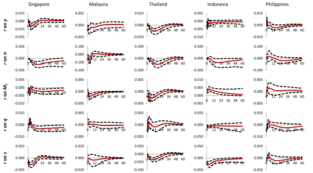
Responses of Domestic Variables to a Domestic Interest Rate Shock
Shocks to the domestic interest rate are used as a measure of monetary policy shocks for
each country.5 The responses of ASEAN-5 economies to their respective monetary policy
shock are shown in Fig. 2.6 The expected response to tighter monetary policy is higher
interest rates, a fall in money supply and a reduction in aggregate demand and inflationary pressures; see Kim and Roubini (2000) for example. As evident in Fig. 2, the M1 responses of Singapore, Malaysia and Thailand are consistent with this expectation while for the Philippines M1 was not significantly affected and for Indonesia a liquidity puzzle is present where M1 increases instead of falling.
In all five economies, the responses of output and inflation to an interest rate shock are as expected; there is no evidence of an output or price puzzle. An unanticipated positive interest rate shock causes output to decline, with an immediate and transitory response lasting for less than a year, although in Indonesia, Malaysia and the Philippines the effects are largely insignificant. The inflationary response is negative in four of the countries, and insignificant for the Philippines, but varies greatly in length. In Singapore the deflationary response is significant out to 4 years, while in Malaysia the response is quite short-lived, dissipating in about one year, whereas Thailand is between these two. While the Indonesian response is largely negative, it is insignificant for most horizons, a feature also of the response in the Philippines. Importantly, however, there is no evidence of significant price puzzle in any of these economies.
The rise in interest rate followed by a fall in inflation, leads to a rise the real interest rate and a short lived appreciation of the real exchange rate observed in all economies except
5 Singapore’s monetary policy is centred on the foreign exchange rate; where the exchange rate is allowed to
appreciate or depreciate depending on factors such as the level of world inflation and domestic price pressures.
6
For comparative purposes, responses of Singapore variables to the exchange rate are shown in Fig. 1B, Appendix B - the negative responses of y and π to an positive (appreciation) q shock are as expected; there is no evidence of output or price puzzles.
17 Indonesia. An unanticipated tightening of monetary policy also depresses the stock market of all economies with immediate effect (although the Philippines experience an insignificant positive bounce within the first quarter). Following the implementation of contractionary monetary policy, the results are consistent with a rise in borrowing costs, temporary fall in output and increase in the discount rate of dividends leading to a fall in real stock prices.
One interesting point to note is that in all economies, the fall in real stock prices was greater than the fall in output growth, indicating that an interest rate shock could be used to offset upswings in the stock prices in ASEAN-5 economies without substantially depressing output growth. However, the same cannot be said about inflation, as the fall in the inflation rate is greater than the fall in real stock prices, suggesting that if stock market imbalances are falsely identified, responding to them through monetary policy could induce undesirable consequences for inflation. On the other hand, a price stability focussed monetary policy may
not be strong enough to contain stock market fluctuations.7
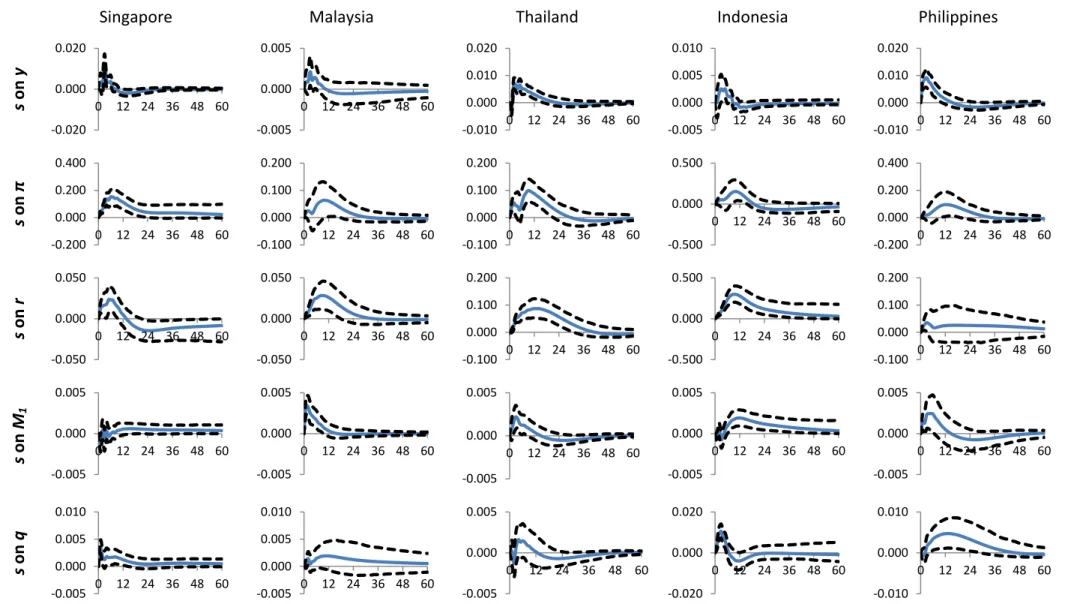
Responses of Domestic Variables to a Stock Price Shock
Fig. 3 shows the responses of ASEAN-5 economies to a positive shock in their domestic stock market. In all economies, output, inflation and monetary aggregate respond positively (although the Singaporean M1 response is insignificant and rather poorly estimated) – reflecting a rise in consumption through the wealth effect and investment through a Tobin Q effect. The stock price channel seems to play an important role in the transmission mechanism in this region, where a monetary easing (tightening) causes stock prices to rise (fall), as evidenced in the previous section, which in turn causes output, inflation and
monetary aggregate to rise (fall).8
7
Similar outcome is also observed for Singapore using exchange rate as the monetary policy variable, see Fig. 1B, in Appendix B.
8
This is consistent withRaghavan et el. (2012), who found that in the post-Asian crisis period, the stock price channel plays an important role in the Malaysian monetary policy transmission mechanism.
18 Interest rates increase immediately following a positive shock in real stock prices, implying that a stock price movement is an important indicator for monetary policy setting in these economies. A rise in the interest rate is followed by an appreciation of the domestic currency.
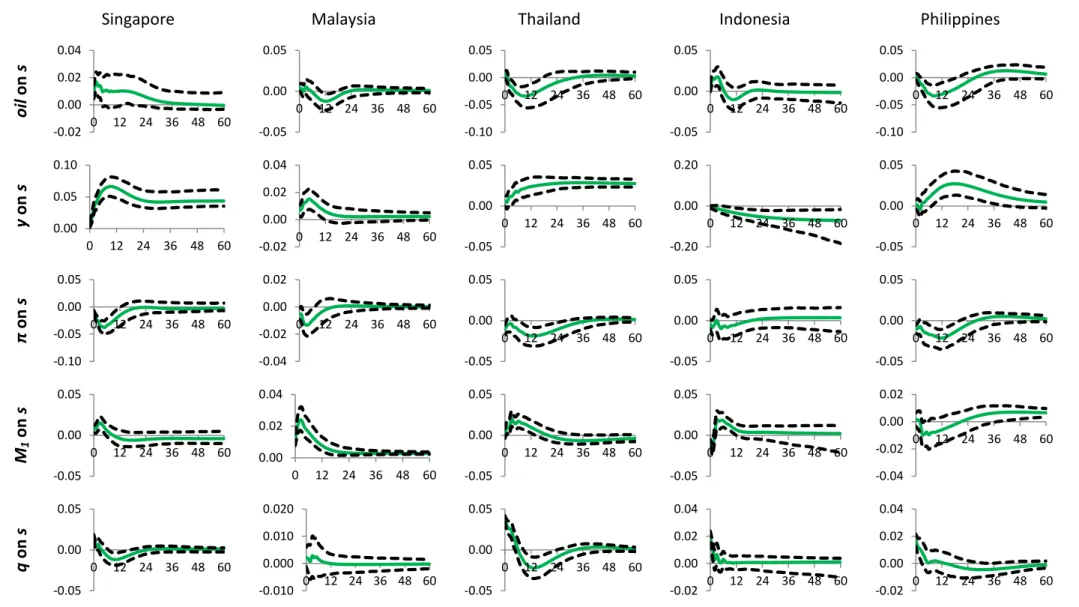
Responses of Real Stock Prices to Foreign and Domestic Shocks
The responses of real stock prices of the ASEAN-5 to shocks originating from the foreign sector and elsewhere in the own economies are reported in Fig. 4. In Thailand and the Philippines increases in oil price inflation led to a negative response in stock prices reflecting the importance of oil as a production input and that these countries are oil importers. Stock prices in Malaysia are insignificantly higher, while in Singapore and Indonesia they are significantly higher. Malaysia and Indonesia are both oil exporters, and Indonesia is the second largest oil producer in the Asian region (after China) and produces large amounts of natural gas, while Singapore plays a major role in global oil refinery and
distribution. The higher stock prices resulting from an oil price shock reflect the importance
of oil to these economies. Almost one-fifth of the world's oil production is transported via the Malacca Straits and related transport and processing industries account for around 5 percent of Singapore’s GDP.
Positive output shocks also lead to the expected reaction. Improved economic activity buoys stock markets significantly in all markets except Indonesia. It is not clear why the Indonesia equity market is not responding positively to higher output here, but it may reflect concerns about the fiscal sustainability of the government stance. The empirical models reflect the observed reality of the sample data, and during this period the Indonesian government has been operating policies aimed at reducing debt and lengthening the maturity of the yield curve. These policies resulted in capital inflows to the extent that the authorities
19 implemented a plan to maintain financial stability by requiring minimum holding periods in the debt market (Hendar, 2012). These interventions may be responsible for distorting the reaction of the equity market to higher growth - particularly if the shock implemented is most representative of a government expenditure or taxation shock; something which cannot be determined in the current specification, but given the history of the Indonesian economy over the sample period is not an unreasonable supposition. This is scope for future work.
A positive inflationary shock results in lower stock prices, significant in all but Indonesia, indicating that in these economies stock prices have poor hedging properties against inflation, consistent with developing economy phenomenon. Money supply shocks result in increased stock prices in all economies in the short term - although this response is insignificant in the Philippines. Higher liquidity levels are leading to a bullish stock market. Exchange rate shocks, where a positive shock represents an appreciation of the domestic
currency, lead to a short lived increase in stock prices, followed by a fall in stock prices,
albeit insignificant in Malaysia and Indonesia. Reflecting that most of these economies have a strong export sector, any competitive appreciation effects and consequent fall in the value of the domestic economy lead to falls in stock prices.
The responses discussed in this section suggest that the stock market responds most strongly to output and liquidity shocks in each economy, and much less so to monetary policy shocks, potentially implying that monetary policy cannot be effectively directly applied to contain stock market bubbles. On the other hand, changing the liquidity levels in these economies may be a promising avenue to contain exuberance in stock prices. The next section allows us to address this more clearly by directly comparing the contributions of these individual shocks to the evolution of stock prices and interest rates.
20
Singapore Malaysia Thailand Indonesia Philippines
r on y r on π r on M 1 r on q r on s
Fig. 2. Impulse Responses of Domestic Variables to an Interest Rate Shock
-0.020 -0.010 0.000 0.010 0 12 24 36 48 60 -0.002 0.000 0.002 0 12 24 36 48 60 -0.010 0.000 0.010 0 12 24 36 48 60 -0.010 -0.005 0.000 0.005 0 12 24 36 48 60 -0.010 0.000 0.010 0 12 24 36 48 60 -0.500 0.000 0.500 0 12 24 36 48 60 -0.200 -0.100 0.000 0.100 0 12 24 36 48 60 -0.200 0.000 0.200 0 12 24 36 48 60 -0.500 0.000 0.500 0 12 24 36 48 60 -0.200 0.000 0.200 0 12 24 36 48 60 -0.010 -0.005 0.000 0.005 0 12 24 36 48 60 -0.005 0.000 0.005 0 12 24 36 48 60 -0.005 0.000 0.005 0 12 24 36 48 60 -0.005 0.000 0.005 0.010 0 12 24 36 48 60 -0.005 0.000 0.005 0 12 24 36 48 60 -0.010 0.000 0.010 0 12 24 36 48 60 -0.005 0.000 0.005 0 12 24 36 48 60 -0.005 0.000 0.005 0 12 24 36 48 60 -0.050 0.000 0.050 0 12 24 36 48 60 -0.010 0.000 0.010 0 12 24 36 48 60 -0.050 0.000 0.050 0 12 24 36 48 60 -0.020 0.000 0.020 0 12 24 36 48 60 -0.100 -0.050 0.000 0.050 0 12 24 36 48 60 -0.050 0.000 0.050 0 12 24 36 48 60 -0.050 0.000 0.050 0 12 24 36 48 60
21
Singapore Malaysia Thailand Indonesia Philippines
s on y s on π s on r s on M 1 s on q
Fig. 3. Impulse Responses of Domestic Variables to a Real Stock Price Shock
-0.020 0.000 0.020 0 12 24 36 48 60 -0.005 0.000 0.005 0 12 24 36 48 60 -0.010 0.000 0.010 0.020 0 12 24 36 48 60 -0.005 0.000 0.005 0.010 0 12 24 36 48 60 -0.010 0.000 0.010 0.020 0 12 24 36 48 60 -0.200 0.000 0.200 0.400 0 12 24 36 48 60 -0.100 0.000 0.100 0.200 0 12 24 36 48 60 -0.100 0.000 0.100 0.200 0 12 24 36 48 60 -0.500 0.000 0.500 0 12 24 36 48 60 -0.200 0.000 0.200 0.400 0 12 24 36 48 60 -0.050 0.000 0.050 0 12 24 36 48 60 -0.050 0.000 0.050 0 12 24 36 48 60 -0.100 0.000 0.100 0.200 0 12 24 36 48 60 -0.500 0.000 0.500 0 12 24 36 48 60 -0.100 0.000 0.100 0.200 0 12 24 36 48 60 -0.005 0.000 0.005 0 12 24 36 48 60 -0.005 0.000 0.005 0 12 24 36 48 60 -0.005 0.000 0.005 0 12 24 36 48 60 -0.005 0.000 0.005 0 12 24 36 48 60 -0.005 0.000 0.005 0 12 24 36 48 60 -0.005 0.000 0.005 0.010 0 12 24 36 48 60 -0.005 0.000 0.005 0.010 0 12 24 36 48 60 -0.005 0.000 0.005 0 12 24 36 48 60 -0.020 0.000 0.020 0 12 24 36 48 60 -0.010 0.000 0.010 0 12 24 36 48 60
22
Singapore Malaysia Thailand Indonesia Philippines
o il on s y on s π on s M1 on s q on s
Fig. 4. Impulse Responses of Real Stock Prices to Various Shocks
-0.02 0.00 0.02 0.04 0 12 24 36 48 60 -0.05 0.00 0.05 0 12 24 36 48 60 -0.10 -0.05 0.00 0.05 0 12 24 36 48 60 -0.05 0.00 0.05 0 12 24 36 48 60 -0.10 -0.05 0.00 0.05 0 12 24 36 48 60 0.00 0.05 0.10 0 12 24 36 48 60 -0.02 0.00 0.02 0.04 0 12 24 36 48 60 -0.05 0.00 0.05 0 12 24 36 48 60 -0.20 0.00 0.20 0 12 24 36 48 60 -0.05 0.00 0.05 0 12 24 36 48 60 -0.10 -0.05 0.00 0.05 0 12 24 36 48 60 -0.04 -0.02 0.00 0.02 0 12 24 36 48 60 -0.05 0.00 0.05 0 12 24 36 48 60 -0.05 0.00 0.05 0 12 24 36 48 60 -0.05 0.00 0.05 0 12 24 36 48 60 -0.05 0.00 0.05 0 12 24 36 48 60 0.00 0.02 0.04 0 12 24 36 48 60 -0.05 0.00 0.05 0 12 24 36 48 60 -0.05 0.00 0.05 0 12 24 36 48 60 -0.04 -0.02 0.00 0.02 0 12 24 36 48 60 -0.05 0.00 0.05 0 12 24 36 48 60 -0.010 0.000 0.010 0.020 0 12 24 36 48 60 -0.05 0.00 0.05 0 12 24 36 48 60 -0.02 0.00 0.02 0.04 0 12 24 36 48 60 -0.02 0.00 0.02 0.04 0 12 24 36 48 60
23
Historical Decomposition
Fig. 5 depicts the contribution of foreign and domestic interest rate shocks, inflation and stock market shocks to interest rates in each of the 5 economies. It is immediately evident
that US interest rate shocks play a substantial role for all but Malaysia. As in Raghavan et al.
(2012), we contend that the fixed exchange rate regime of Malaysia and capital account control measures in place, shelters domestic interest rates from these effects. The more flexible exchange rate regimes in the remaining countries make them more responsive to international financial conditions. In most cases, the foreign interest rate shocks, representing international financial conditions, outweigh the contributions of domestic interest rate shocks. This is unlike a number of small open economies with developed financial markets, where domestic interest rates tend to be determined more closely in response to domestic conditions - for example Australia, the US, the Euro Area in Dungey and Pagan (2000), Dungey and
Osborn (2013), Dungey et al. (2013). It may also reflect the more export-oriented focus of
these growing Asian economies.
Domestic interest rate shocks are particularly important in Malaysia and the Philippines in the early part of the sample. Inflation shocks contribute more than shocks originating from output, money supply or exchange rates (not shown), but are not dominant in determining the interest rate in any country. The focus of this paper is on the interaction between stock markets and interest rates, as shown in the last row of Fig. 5, stock market shocks make a relatively small contribution to the determination of interest rates in all of the countries examined.
Fig. 6 shows the contributions of shocks to oil, foreign and domestic interest rates and stock markets to the evolution of stock market variables in each economy. As with the analysis of interest rates in Fig. 5, here shocks to foreign interest rates - which represent international financial conditions - have an important role in driving the stock markets in
24 most countries. Malaysia is again an exception, reflecting its capital controls and fixed exchange rate regime. The contribution of the international financial shocks is highest for the affected countries in the 2005-2008 periods, in the lead up to the Global Financial Crisis.
Oil price shocks make a notable contribution to the stock prices for Malaysia and Indonesia, two oil exporting economies, and also to the Philippines and Thailand, two oil importers. Surprisingly, given the importance of oil refining and distribution to the Singaporean economy, the contribution of oil price shocks to stock prices is relatively low - less than that of domestic output or inflation (not shown). The major contribution to stocks prices in each country comes through own shocks. In general, with the exception of Thailand, the contribution of the domestic interest rate shocks to stock prices is quite small.
VI Conclusion
This paper builds a structural VECM model for each of the ASEAN-5 economies that takes account of the mixed stationary and non-stationary variables and determine the co-integration relationship that exists between the integrated series. We find that real stock market indices are typically cointegrated with measures of macroeconomic activities such as the real output, money stock and exchange rate. The presence of a cointegrating relationship between macroeconomic variables and the stock prices indicates long run behaviour of the stock market and it provides incremental information about the stock price dynamics.
Using developing economy application, we establish identification conditions on the contemporaneous matrix to uncover the dynamic effects of the orthogonal policy and stock price shocks to assess the impact of monetary policy shocks on stock prices and vice versa. The impulse responses and historical decomposition generated for each of the ASEAN-5 countries enable us to assess whether monetary policy has a pronounced effect on the stock market of these economies. Monetary policy focused on the stock market could be
25 incompatible with the price stability objective in these economies because while aiming to contain stock market bubble, they may inadvertently depress the output and inflation which would lead to slowdown of these economies. Therefore, the monetary authorities of the ASEAN-5 may need to re-evaluate their monetary policy if leaning against the stock market is something they desire. In contrast, a price stability focused monetary policy may not be sufficient to avoid or control large stock market price fluctuations. Managing the liquidity levels may be a promising avenue to the ASEAN-5 economies to contain any exuberance in stock prices.
As indicated by Boivin et al. (2010), Mishkin (2011) and Gali (2013), if price stability is
not a sufficient condition for financial stability, then other policy instruments should be sought to attain financial stability. The ASEAN-5 policy makers should continue to use monetary policy to achieve price and output stability while at the same time strengthening their financial supervision and prudential regulation to constrain any future asset price bubbles in these economies. The current work thus can be extended to assess the interaction between monetary policy and macro-prudential policy of the ASEAN-5 in containing undesirable movements in stock prices while maintaining price stability. This is a scope for future work.
26 Fig. 5. Historical Decomposition of Domestic Interest Rate to Various Shocks
-1.00 -0.50 0.00 0.50 1.00 1.50 M ay -0 0 Ma y -0 1 Ma y -0 2 Ma y -0 3 M ay -0 4 M ay -0 5 M ay -0 6 M ay -0 7 M ay -0 8 M ay -0 9 M ay -1 0 M ay -1 1 Singapore -0.80 -0.60 -0.40 -0.20 0.00 0.20 0.40 0.60 0.80 Ma y -0 0 M ar-0 1 Ja n -0 2 No v -0 2 S ep -0 3 Ju l-0 4 M ay -0 5 M ar-0 6 Ja n -0 7 No v -0 7 S ep -0 8 Ju l-0 9 M ay -1 0 M ar-1 1 Malaysia -2.00 -1.50 -1.00 -0.50 0.00 0.50 1.00 1.50 2.00 M ay -0 0 M ar-0 1 Ja n -0 2 No v -0 2 S ep -0 3 Ju l-0 4 M ay -0 5 Ma r-0 6 Ja n -0 7 No v -0 7 S ep -0 8 Ju l-0 9 M ay -1 0 M ar-1 1 Thailand -3.00 -2.00 -1.00 0.00 1.00 2.00 3.00 4.00 5.00 6.00 Ma y -0 0 M ar-0 1 Ja n -0 2 No v -0 2 S ep -0 3 Ju l-0 4 M ay -0 5 M ar-0 6 Ja n -0 7 No v -0 7 S ep -0 8 Ju l-0 9 M ay -1 0 M ar-1 1 Indonesia -2.00 -1.00 0.00 1.00 2.00 3.00 4.00 5.00 M ay -0 0 M ar-0 1 Ja n -0 2 No v -0 2 S ep -0 3 Ju l-0 4 M ay -0 5 Ma r-0 6 Ja n -0 7 No v -0 7 S ep -0 8 Ju l-0 9 M ay -1 0 M ar-1 1 Philippines
27 Fig. 6. Historical Decomposition of Real Stock Prices to Various Shocks
-0.40 -0.30 -0.20 -0.10 0.00 0.10 0.20 0.30 May-00 Ap r-01 Mar -02 Fe b -03 Jan-04 Dec-04 Nov-05 Oct -06 Se p -07 A u g-08 Ju l-09 Ju n -10 M ay-11 Singapore -0.20 -0.15 -0.10 -0.05 0.00 0.05 0.10 0.15 0.20 0.25 0.30 May-00 Ap r-01 Mar -02 Fe b -03 Jan-04 Dec-04 Nov-05 Oct -06 Se p -07 A u g-08 Ju l-09 Ju n -10 M ay-11 Malaysia -0.40 -0.30 -0.20 -0.10 0.00 0.10 0.20 0.30 0.40 May-00 Ap r-01 Mar -02 Fe b -03 Jan-04 Dec-04 Nov-05 Oct -06 Se p -07 A u g-08 Ju l-09 Ju n -10 M ay-11 Thailand -0.40 -0.30 -0.20 -0.10 0.00 0.10 0.20 0.30 May-00 Ap r-01 Mar -02 Fe b -03 Jan-04 Dec-04 Nov-05 Oct -06 Se p -07 A u g-08 Ju l-09 Ju n -10 M ay-11 Indonesia -0.40 -0.30 -0.20 -0.10 0.00 0.10 0.20 0.30 May-00 Ap r-01 Mar -02 Fe b -03 Jan-04 Dec-04 Nov-05 Oct -06 Se p -07 A u g-08 Ju l-09 Ju n -10 M ay-11 The Philippines
28 References
Adrian, T. and H. Y. Shin (2010) Financial Intermediaries and Monetary Economics, Federal Reserve Bank of New York, Staff reports, 398.
Allen, F. and K. Rogoff (2011) Asset Prices, Financial Stability and Monetary Policy, http://fic.wharton.upenn.edu/fic/papers/11/11-39.pdf
Asprem, M. (1989) Stock Prices, Asset Portfolios and Macroeconomic Variables in Ten
European Countries, Journal of Banking and Finance, 13, 589-612.
Bean, C., M. Paustian, A. Penalver and T. Taylor (2010) Monetary Policy after the Fall,
Federal Reserve Bank of Kansas City Annual Conference.
Bernanke, B. S. And M. Gertler (2001) Should Central Banks Respond to Asset Prices?
American Economic Review,91, 253-257.
Bernanke, B. S. and K. N. Kuttner (2005) What Explains the Stock Market’s Reaction to
Federal Reserve Policy?, The Journal of Finance, 60, 1221-1256.
BNM (1994) Money and Banking in Malaysia, Kuala Lumpur.
BNM (1999) The Central Bank and the Financial System in Malaysia: A Decade of Change,
Kuala Lumpur.
Bjorland, C. and K. Leitemo (2009) Identifying the Interdependence between US Monetary
Policy and the Stock Market, Journal of Monetary Economics,56, 275-282.
Boivin, J., T. Lane and C. Meh (2010) Should Monetary Policy be used to Counteract
Financial Imbalances? Bank of Canada Review
Bordo, M., B. Eichengreen, D. Klingebiel, M. Martinez-Peria, and A. Rose (2001) Is The
Crisis Problem Growing More Severe?, Economic Policy16, 53-82.
Cassola, N. and C. Morana (2002) Monetary Policy and the Stock Market in the Euro Area, European Central Bank Working Paper Series, 119.
29 Cheung, Y.W. and L.K. Ng (1998) International Evidence on the Stock Market and
Aggregate Economic Activity, Journal of Empirical Finance,5, 281-296.
Cecchetti, S., H. Genberg, J. Lipsky and S. Wadhwani (2000) Asset Prices and Central Bank Policy, The Geneva Report on the World Economy, 2, ICMB/CEPR.
Cushman, D. O. and T. A. Zha (1997) Identifying Monetary Policy in a Small Open
Economy Under Flexible Exchange Rates, Journal of Monetary Economics, 39, 433-448.
D’Amico S. and M. Farka (2011) The Fed and the Stock market:An Identificatio Based on
Intraday Futures Data, Journal of Business and Economics Statistics, 29, 126-137.
Dungey, M. and D. R. Osborn (2013) Modelling large open economies with international
linkages: The US and Euro Area, Journal of Applied Econometrics, doi:10.1002/jae.2323
Dungey, M., D. R. Osborn and M. Raghavan (2013) International Transmissions to Australia: The Roles of the US and Euro Area, UTAS Discussion Paper 2013-10.
Dungey, M. and A. R. Pagan (2000) A Structural VAR Model of the Australian Economy,
Economic Record, 76, 321-342.
Dungey, M. and A. R. Pagan (2009) Extending a SVAR Model of the Australian Economy,
Economic Record, 85, 1-20.
Fisher, L. A. and H. S. Huh, (2012) Identification Methods in Vector-Error Correction
Models: Equivalence Results, Journal of Economic Survey, doi:
10.1111/j.1467-6419.2012.00734.x
Gali, J. (2013) Monetary Policy and Rational Asset Price Bubbles, NBER Working Paper 18806.
Goodhart, C. and B. Hofmann (2000) Do Asset Price Help to Predict Consumer Price
Inflation?, Manchester School, 68, 122-140.
Gordon, M. J. (1962) The Investment, Financing and Valuation of Corporation, Irwin,
30
Gurkaynak, S. (2008) Econometric Tests of Asset Price Bubbles: Taking Stock, Journal of
Economic Survey, 22, 166-186.
Hendar, M. (2012) Fiscal Policy, Public Debt Management and Government Bond Markets in Indonesia, in Fiscal Policy, Public Debt and Monetary Policy in Emerging Market
Economies, BIS Papers no. 67, October, 199-203.
Hong, K. and H. C. Tang (2010) Crises in Asia: Recovery and Policy Responses, Working Paper Series on Regional Economic Integration, Asian Development Bank. 48.
Katrin, A. W. and G. Stefan (2008) Ensuring Financial Stability: Financial Structure and the Impact of Monetary Policy on Asset Prices, C.E.P.R. Discussion Papers, 6773
Kilian, L. (1998) Small-Sample Confidence Intervals for Impulse Response Functions,
Review of Economics and Statistics, 80, 218-230.
Kim, S. And N. Roubini (2000) Exchange rate anomalies in the industrial countries: A
solution with a structural VAR approach, Journal of Monetary Economics, 45, 561-586.
Kim, S. and D.Y. Yang (2012) International Monetary Transmission in East Asia: Floaters,
Non-floaters and Capital Controls, Japan and the World Economy,
doi:10.1016/j.japwor.2012.05.003
Kohn, D. L. (2009) Monetary Policy and Asset Prices Revisited, CATO Journal, 29, 31-44.
Kohn, D. L. (2006) Monetary Policy and Asset Prices, Speech at Monetary Policy: A Journey
from Theory to Practice, European Central Bank Colloquium in honor of Otmar Issing. Kuttner, K.N. (2011) Monetary Policy and Asset Price Volatility: Should We Refill the
Bernanke-Gertler Prescription? Working Papers 2011-04, Department of Economics, Williams College.
Laeven, L. and F. Valencia (2012) The Use of Blanket Guarantees in Banking Crises, Journal
31 Lastrapes, W.D. (1998) International Evidence on Equity Prices, Interest Rates and Money,
Journal of International Money and Finance, 17, 377- 406.
Lee, B. S. (1992) Causal Relations among Stock Returns, Interest Rates, Real Activity and
Inflation, The Journal of Finance,47, 1591-1603.
Mandelker, G. and K. Tandon (1985) Common Stock Returns, Real Activity, Money and
Inflation: Some International Evidence, Journal of International Money and Finance, 4,
267-286.
Millard, S. P. And S. Wells (2003) The Role of Asset Prices in Transmitting Monetary and Other Shocks, Bank of England Working Paper, 188.
Mishkin, F. S (2011) Over the Cliff: From the Subprime to the Global Crisis, NBER Working
Paper,16609.
Muradoglu, G., K. Metin and R. Argac (2001) Is there a Long Run Relationship between Stock Returns and Monetary Variables: Evidence from an Emerging market, Applied
Financial Economics, 11, 641-650
Neri, S. (2004) Monetary Policy and Stock Prices, Bank of Italy Working Paper, 513.
Patelis, A.D. (1997) Stock Return Predictability and the Role of Monetary Policy, The
Journal of Finance, 52, 1951-1972.
Pagan, A. R. and Pesaran, M. H. (2008) Econometric analysis of structural systems with
permanent and transitory shocks, Journal of Economic Dynamics and control, 32,
3376-3395.
Raghavan, M., P. Silvapulle, and G. Athanasopoulos (2012). Structural VAR Models for Malaysian Monetary Policy Analysis during the Pre- and Post-1997 Asian Crisis Periods.
Applied Economics 44, 3841-3856.
Rapach, D.E. (2001) Macro Shocks and Real Stock Prices, Journal of Economics and
32
Reinhart, C. R. and K. S. Rogoff (2009) This Time is Different – Eight Centuries of Financial
Folly, Princeton University Press.
Sack, B. and V. Weiland (2000) Interest-rate Smoothing and Optimal Monetary Policy: A
Review of Recent Empirical Evidence, Journal of Economics and Business, 52, 205-228.
Shimada, T. and T. Yang (2010) Challenges and Developments in the Financial Systems of
the Southeast Asian Economies, OECD Journal: Financial Market Trends, 2.
Sims, C. A. (1992) Interpreting the Macroeconomic Time Series Facts; The Effects of
Monetary Policy, European Economic Review, 36, 975-1011.
Thorbecke, W. (1997) On Stock Market Returns and Monetary Policy, The Journal of
Finance, 52, 635-654.
White, W. R (2009) Should Monetary Policy Lean or Clean?, Globalization and Monetary Policy Institute Working Paper, 34
Wongbangpo, P. and S. Sharma (2002) Stock Market and Macroeconomic Fundamental
Dynamic Interactions: ASEAN-5 Countries, Journal of Asian Economics, 13, 27-51
33
Appendix A:
Table 1A. Data Descriptions and Sources
Data Description Source
oil Oil Prices Spot Oil Price: West Texas
Intermediate, FRED Database
r* Federal Funds Rate (percentage) IFS, Federal Reserve Website
y Industrial Production (SA), Logs, Datastream
π CPI (percentage change per annum) IFS, Datastream
r Overnight Interbank/Treasury Bills Rate (percentage)
IFS, Datastream, Respective Central Bank Websites
M1 Monetary Aggregregate M1 (SA),Logs IFS, Datastream
q Real Exchange Rate (nominal exchange rate as local currency per unit of foreign
currency times the ratio of foreign and domestic CPIs); Logs
IFS, Datastream, Respective Central Bank Websites
s Real Stock Price Index IFS, Datastream, Yahoo Finance
Table 2A. Augmented Dickey-Fuller Unit Root Test Results
Levels oil r*
ADF Stat -4.629 -3.678
p-value 0.000* 0.006*
Levels y π r M1 q s
Singapore ADF Stat -2.766 -2.716 -1.768 -0.909 -0.032 -2.061
p-value 0.213 0.074** 0.395 0.951 0.959 0.261 Malaysia ADF Stat -1.987 -3.112 -2.421 -3.143 -0.358 -1.307
p-value 0.603 0.028* 0.138 0.101 0.912 0.626 Thailand ADF Stat -0.743 -2.253 -2.266 -1.754 -1.193 -1.486
p-value 0.967 0.189 0.185 0.722 0.676 0.537 Indonesia ADF Stat -2.572 -2.975 -1.765 -0.691 -3.101 -0.782
p-value 0.293 0.039* 0.398 0.971 0.108 0.821 Philippines ADF Stat -3.134 -3.721 -1.771 -2.587 -0.394 -1.063
p-value 0.102 0.005* 0.393 0.287 0.906 0.729 Notes: ADF is the conventional Augmented Dickey-Fuller test, with augmentation selected by AIC with a maximum of 12 lags. . Tests for y and M1 allow an intercept and trend; all others allow an intercept only. * and ** indicates the statistic is significant at 5% and 10% respectively.
34 Table 3A. Johansen Cointegration Tests
VAR for y, M1, q and s
Trace Test H0: n=0 H0: n=1 H0: n=2 Singapore 0.000 0.031 0.122 Malaysia 0.000 0.005 0.103 Thailand 0.000 0.087 0.331 Indonesia 0.000 0.007 0.155 Philippines 0.001 0.006 0.192
Notes: Four lagged differences and unrestricted intercepts are included in the VAR models. Results are shown p-values in relation to the null hypothesis for the presence of n= 0, 1 or 2 cointegrating relationship.
Table 4A. Residual Correlations
oil r* y π r M1 q s Singapore r -0.024 0.017 -0.036 -0.003 1.000 -0.059 -0.012 0.000 s 0.000 0.000 0.000 0.000 0.000 0.000 0.000 1.000 Malaysia r -0.081 -0.048 -0.064 0.013 1.000 0.038 -0.023 0.000 s 0.000 -0.001 0.000 0.000 0.000 0.000 0.000 1.000 Thailand r -0.008 0.012 -0.030 0.031 1.000 -0.016 0.010 0.000 s 0.000 0.000 0.000 0.000 0.000 0.000 0.000 1.000 Indonesia r -0.080 -0.050 -0.037 -0.024 1.000 -0.046 -0.003 0.000 s 0.000 0.000 0.000 0.000 0.000 0.000 0.000 1.000 Philippines r 0.056 -0.003 0.046 -0.029 1.000 -0.026 -0.007 0.000 s 0.000 0.000 0.000 0.000 0.000 0.000 0.000 1.000
Table 5A. Size of One SD Shocks
oil r* y π r M1 q s Singapore 13.717 0.422 0.064 0.484 0.186 0.014 0.014 0.043 Malaysia 13.717 0.422 0.020 0.514 0.080 0.013 0.011 0.038 Thailand 13.717 0.422 0.046 0.526 0.193 0.016 0.016 0.049 Indonesia 13.717 0.422 0.039 1.137 0.324 0.009 0.026 0.049 Philippines 13.717 0.422 0.034 0.387 0.356 0.013 0.017 0.051
35
Appendix B:
Fig.1B. Impulse Responses of Singaporean Variables to an Exchange Rate Shock
-0.01 -0.005 0 0.005 0.01 0 12 24 36 48 60 q on y -0.3 -0.2 -0.1 0 0.1 0 12 24 36 48 60 q on π -0.1 -0.05 0 0.05 0 12 24 36 48 60 q on r -0.005 0 0.005 0.01 0 12 24 36 48 60 q on M1 -0.01 0 0.01 0.02 0 12 24 36 48 60 q on q -0.04 -0.02 0 0.02 0.04 0 12 24 36 48 60 q on s
TASMANIAN
S
CHOOL
OF
BUSINESS
AND
E
CONOMICS
WORKING
PA
P
ER
S
ERIES
2014-08 How Many Stocks are Enough for Diversifying Canadian Institutional Portfolios? Vitali Alexeev and Fran-cis Tapon
2014-07 Forecasting with EC-VARMA Models, George Athanasopoulos, Don Poskitt, Farshid Vahid, Wenying Yao
2014-06 Canadian Monetary Policy Analysis using a Structural VARMA Model, Mala Raghavan, George Athana-sopoulos, Param Silvapulle
2014-05 The sectorial impact of commodity price shocks in Australia, S. Knop and Joaquin Vespignani
2014-04 Should ASEAN-5 monetary policymakers act pre-emptively against stock market bubbles? Mala
Raghavan and Mardi Dungey
2014-03 Mortgage Choice Determinants: The Role of Risk and Bank Regulation, Mardi Dungey, Firmin Doko Tchatoka, Graeme Wells, Maria B. Yanotti
2014-02 Concurrent momentum and contrarian strategies in the Australian stock market, Minh Phuong Doan,
Vi-tali Alexeev, Robert Brooks
2014-01 A Review of the Australian Mortgage Market, Maria B. Yanotti
2013-20 Towards a Diagnostic Approach to Climate Adaptation for Fisheries, P. Leith, E. Ogier, G. Pecl, E. Hoshino, J. Davidson, M. Haward
2013-19 Equity Portfolio Diversification with High Frequency Data, Vitali Alexeev and Mardi Dungey
2013-18 Measuring the Performance of Hedge Funds Using Two-Stage Peer Group Benchmarks, Marco Wilkens, Juan Yao, Nagaratnam Jeyasreedharan and Patrick Oehler
2013-17 What Australian Investors Need to Know to Diversify their Portfolios, Vitali Alexeev and Francis Tapon 2013-16 Equity Portfolio Diversification: How Many Stocks are Enough? Evidence from Five Developed Markets,
Vitali Alexeev and Francis Tapon
2013-15 Equity market Contagion during the Global Financial Crisis: Evidence from the World’s Eight Largest Econ-omies, Mardi Dungey and Dinesh Gajurel
2013-14 A Survey of Research into Broker Identity and Limit Order Book, Thu Phuong Pham and P Joakim Westerholm
2013-13 Broker ID Transparency and Price Impact of Trades: Evidence from the Korean Exchange, Thu Phuong Pham
2013-12 An International Trend in Market Design: Endogenous Effects of Limit Order Book Transparency on Vola-tility, Spreads, depth and Volume, Thu Phuong Pham and P Joakim Westerholm