Detecting Outliers in High-Dimensional Neuroimaging
Datasets with Robust Covariance Estimators
Virgile Fritsch, Ga¨
el Varoquaux, Benjamin Thyreau, Jean-Baptiste Poline,
Bertrand Thirion
To cite this version:
Virgile Fritsch,
Ga¨
el Varoquaux,
Benjamin Thyreau,
Jean-Baptiste Poline,
Bertrand
Thirion.
Detecting Outliers in High-Dimensional Neuroimaging Datasets with Robust
Covariance Estimators.
Medical Image Analysis,
Elsevier,
2012,
16,
pp.1359-1370.
<
10.1016/j.media.2012.05.002
>
.
<
hal-00701225
>
HAL Id: hal-00701225
https://hal.inria.fr/hal-00701225
Submitted on 24 May 2012
HAL
is a multi-disciplinary open access
archive for the deposit and dissemination of
sci-entific research documents, whether they are
pub-lished or not.
The documents may come from
teaching and research institutions in France or
abroad, or from public or private research centers.
L’archive ouverte pluridisciplinaire
HAL, est
destin´
ee au d´
epˆ
ot et `
a la diffusion de documents
scientifiques de niveau recherche, publi´
es ou non,
´
emanant des ´
etablissements d’enseignement et de
recherche fran¸
cais ou ´
etrangers, des laboratoires
publics ou priv´
es.
Detecting Outliers in High-Dimensional Neuroimaging Datasets with
Robust Covariance Estimators
Virgile Fritscha,c, Ga¨el Varoquauxb,a,c, Benjamin Thyreauc, Jean-Baptiste Polinec,a, Bertrand Thiriona,c a
Parietal Team, INRIA Saclay-ˆIle-de-France, Saclay, France b
Inserm, U992, Neurospin bˆat 145, 91191 Gif-Sur-Yvette, France c
CEA, DSV, I2
BM, Neurospin bˆat 145, 91191 Gif-Sur-Yvette, France
Abstract
Medical imaging datasets often contain deviant observations, the so-called outliers, due to acquisition or preprocessing artifacts or resulting from large intrinsic inter-subject variability. These can undermine the statistical procedures used in group studies as the latter assume that the cohorts are composed of homoge-neous samples with anatomical or functional features clustered around a central mode. The effects of outlying subjects can be mitigated by detecting and removing them with explicit statistical control. With the emer-gence of large medical imaging databases, exhaustive data screening is no longer possible, and automated outlier detection methods are currently gaining interest. The datasets used in medical imaging are often dimensional and strongly correlated. The outlier detection procedure should therefore rely on high-dimensional statistical multivariate models. However, state-of-the-art procedures, based on the Minimum Covariance Determinant (MCD) estimator, are not well-suited for such high-dimensional settings. In this work, we introduce regularization in the MCD framework and investigate different regularization schemes. We carry out extensive simulations to provide backing for practical choices in absence of ground truth knowl-edge. We demonstrate on functional neuroimaging datasets that outlier detection can be performed with small sample sizes and improves group studies.
Keywords: Outlier detection, Minimum Covariance Determinant, regularization, robust estimation, neuroimaging, fMRI, high-dimension
1. Introduction
Medical image acquisitions are prone to a wide va-riety of errors such as scanner instabilities, acquisi-tion artifacts, or issues in the underlying bio-medical experimental protocol. In addition, due to the high variability observed in populations of interest, these datasets may also contain uncommon, yet technically correct, observations. The inclusion of overly noisy or aberrant images in medical datasets typically results
Email address: virgile.fritsch@inria.fr(Virgile Fritsch)
in additional analysis and interpretation challenges. In both cases, images deviating from normality are calledoutliers. Outliers may be numerous, especially in neuroimaging, where the between-subjects vari-ability of anatomical and functional features is very high and images can have a low signal-to-noise ratio. Considering the dramatic influence of outliers in stan-dard statistical procedures such as Ordinary Least Squares regression [12,26], clustering [3,7], manifold learning [37] or neuroimaging group analyzes [16,18], it is crucial to detect outliers as a preprocessing step of any statistical study. Once labeled as such, outly-ing observations can be down-weighted or even
dis-carded in group studies. Down-weighting requires a measure of the deviation from normality for each ob-servation and the rejection of obob-servations must be grounded on a statistical control. Furthermore, an automatic procedure for data screening is also nec-essary in the case of a large number of observations and to avoid subjective bias.
An intrinsic difficulty of outlier detection in med-ical imaging lies in the lack of formal definition for abnormal data; in particular, no generative model for outliers might be sufficient to model the variety of situations where such data are observed in practice. Moreover, in high-dimensional settings, i.e. when the number of observations is less than five times the number of data descriptors (orfeatures) [9], the prob-lem of outlier detection is ill-posed since it becomes very difficult to characterize deviations from normal-ity. From a practical perspective, manual outlier de-tection is impossible in such a situation. Current methods dealing with outliers in a high-dimensional context are essentially univariate methods, i.e. they consider different dimensions one by one [22, 39]. These methods may fail to tag as outliers observa-tions that are deviant with respect to a combination of several of their characteristics, but for which each descriptor considered individually does not reveal de-viation from normality. Medical imaging data, and in particular neuroimaging data, are high dimensional, the underlying dimension being the number of de-grees of freedom in their variance, which can be of the order of the number of image voxels. This is typically much larger than the number of available samples. In functional MRI studies, neuroscientists often screen the data manually (see e.g. [24]), because of the lack of an adapted outlier detection framework. The crite-ria for discarding data are not always quantitatively defined. For instance, images may be discarded if, upon visual inspection, they are not reflecting the expected brain activation pattern (e.g. in a so called contrast map). Such a process is tedious and unre-liable, but most importantly it makes the statistical analysis of the group data invalid for that pattern – as it implies that the variance of this pattern will be underestimated.
In this contribution, we explore several extensions to the state-of-the-art outlier detection framework
of [26] to high-dimensional settings. In particular, we introduce and compare three procedures, all based on a robust and regularized covariance estimate. Using a covariance estimate relies on the assumption that reg-ular observations, called theinliers, are Gaussian dis-tributed, and that outliers are characterized by some distance to the standard model. We simulate vari-ous scenarii that result in outliers by using mixture models, where the location and covariance parame-ters of the outliers component are chosen according to three different outlier models. We focus mostly on the accuracy of outlier detection procedures, and only address the challenging question of exact statis-tical control through simulation procedures; impor-tantly, our choice of a parametric approach facilitates this control. Eventually, we compare our parametric approach to a non-parametric procedure, the One-Class Support Vector Machine (One-One-Class SVM) al-gorithm, since this method has raised much interest recently [8,19].
The layout of the paper is the following. In Sec-tion 2, we present the state-of-the-art outlier detec-tion framework, comprising a robust estimator of lo-cation and covariance, theMinimum Covariance De-terminant (MCD) [25], and we point out its limita-tions in our context. We then introduce in Section3
three new robust covariance estimators derived from the MCD but suitable for high-dimensional settings. In Section4, we present experiments on simulations that we use to assess the performance of our new outlier detection methods, together with the corre-sponding results. Experiments on anatomical and functional neuroimaging datasets are then described in Section 5. Finally, in Section 6, we discuss the results in the context of statistical inference in func-tional neuroimaging group studies.
Notations. We write vectors with bold letters, a ∈
Rn, matrices with capital bold letters,A∈Rn×n. I is the identity matrix. 0and1are constant matrices filled respectively with 0 and 1. Quantities estimated from the data at hand are written with a hat, e.g.
b
A. ATis the transposed matrix andA−1is the
ma-trix inverse ofA. We call the inverse of a covariance matrix the precision matrix. X refers to an n×p matrix representing a dataset ofnobservations
rep-resented bypfeatures. Considering a set of integers H, we denoteXH the matrix (xi j)i∈H, j∈[1..p]. κ(A)
is the condition number of the matrixA, defined by σmax(A)
σmin(A),σmax(A) andσmin(A) being respectively the
largest and the smallest eigenvalues ofA. chol(A) is the lower triangular matrix obtained by the Cholesky decomposition ofA.
2. Detecting outlying observations: state of art procedures
2.1. MCD estimator: robust location and covariance estimates
Assuming a high-dimensional Gaussian model, an observationxi∈Rpwithin a setXcan be character-ized as outlier whenever it has a large Mahalanobis distance to the mean of the data distribution, defined as d2µ,Σ(xi) = (xi−µ)TΣ
−1(x
i−µ), µand Σ be-ing respectively the dataset location and covariance. Crucially, robust estimators of location and covari-ance must be used to compute these distcovari-ances [2,23]. The state-of-the-art robust covariance estimator for multidimensional Gaussian data is Rousseeuw’s Minimum Covariance Determinant (MCD) estima-tor [25]. Given a dataset with n p-dimensional ob-servations,X ∈Rn×p, MCD aims at findingh obser-vations considered as inliers, by minimizing the de-terminant of their scatter matrix. We refer to these observations as thesupport of the MCD.
The core procedure commonly used to compute the MCD estimate of the covariance of a population is given in Algorithm 1. It consists of alternatively choosing a subsetXH ofhobservations to minimize a Mahalanobis distance, and updating the covariance matrix ˆΣH used to compute the Mahalanobis dis-tance. |ΣˆH|decreases at each update of XH. Stan-dard algorithms such as the Fast-MCD algorithm [27] perform this simple procedure several times from dif-ferent initial subsets XH and retain only the solu-tion with the minimal determinant. The MCD can be understood as an alternated optimization of the
following problem: ( ˆH,µˆh,Σˆh) = argmin µ,Σ,H log|Σ| +1 h X i∈H (xi−µ)TΣ−1(xi−µ) , (1)
The limitations of the MCD come from the fact that the scatter matrix must be full rank, as it is used to define a Mahalanobis distance. As a consequence, h must be greater than hmin = n+p2+1: the MCD
cannot learn the inlier distribution if there are less thanhmininliers. In high-dimensional settings, as pn
becomes large,hminincreases and outliers are
poten-tially included in the covariance estimation if there are more than n−p−2 1 of them. Whenp=n−1, the MCD estimator is equivalent to the unbiased maxi-mum likelihood estimator, which is not robust. Fi-nally, if p ≥ n, the MCD estimator is not defined. To address these issues we propose to use half of the observations in the support (h = n
2) and
compen-sate the shortage of data for covariance estimation with regularization, referred to as Regularized MCD in the remainder of the text.
2.2. One class SVM: a non-parametric procedure
Medical imaging data is not necessarily well de-scribed by a Gaussian distribution. Thus it might be profitable to seek decision rules not based on Ma-halanobis distances to screen deviant data. For this, we use theOne-Class Support Vector Machine (One-Class SVM) [29], which is not limited by any prior shape of the separation between in- and outlying ob-servations. This choice was motivated by the fact that other robust, high-dimensional, non-parametric tools such as Robust PCA [13] or Local Component Analysis [28] have not yet been considered in prac-tical applications. The One-Class SVM algorithm solves the following quadratic program:
min w∈F,ξ∈Rn,ρ∈ R 1 2kwk 2+ 1 ν n X i ξi−ρ (2) subject to (w·Φ(xi))≥ρ−ξi, ξi≥0 (3) where Φ is a feature mapRp→FverifyingK(x,y) = Φ(x)·Φ(y) for any observationsx,y∈Rpand a given
Algorithm 1MCD estimation algorithm
1. Selecthobservations (call the corresponding datasetXH); 2. Compute the empirical covariance ˆΣ|H and mean ˆµ|H; 3. Compute the Mahalanobis distancesd2
µ|H,Σ|H(xi),i= 1..n;
4. Select thehobservations having the smallest Mahalanobis distance; 5. UpdateXH and repeat steps 2 to 5 until|Σˆ|H| no longer decreases.
kernelK. The important parameter of the One-Class SVM is the margin parameter ν, which is both an upper bound on the proportion of observations that will lie outside the frontier learned by the algorithm and a lower bound on the number of support vectors of the model [29].
In our experiments on simulated data, we setν to the amount of contamination (i.e. the proportion of outliers in the dataset). Note that this choice favors the One-Class SVM compared to methods that ignore the ratio of outliers. For real data experiments, we setν= 0.5 as we work with at most 50% contamina-tion. We use aRadial Basis Function (RBF) kernel and select its inverse bandwidth σ with an heuris-tic inspired by [32]: σ = 0.01
∆ , where ∆ is the 10th
percentile of the pairwise distances histogram of the observations. We verified that this heuristic is close to the optimum parameter on simulations, although the results are not very sensitive to mild variations ofσaround this value.
3. Regularized MCD estimators
To improve upon the classical MCD estimator, we introduce regularization in the MCD estimation pro-cedure.
3.1. ℓ2 regularization (RMCD-ℓ2)
We first investigate outlier detection with estima-tors resulting from a penalized versions of the likeli-hood in Equation 1. This corresponds to replacing the step 2 of the MCD Algorithm 1 by a penalized maximum-likelihood estimate of the covariance ma-trix.
We consider ℓ2 regularization (orridge
regulariza-tion): let λ ∈ R+ be the amount of regulariza-tion, and Σˆr|H the covariance estimate of a n×p
dataset XH that maximizes the penalized negative log-likelihood: ( ˆµr,Σˆr|H) = argmin µ,Σ log|Σ| + 1 h X i∈H (xi−µ)TΣ−1(xi−µ) +λTrΣ−1 , (4) yielding ˆΣr|H = X T HXH h +λI and ˆµr|H = XT H1 h . The covariance estimate is biased toward a spherical co-variance matrix. This bias corresponds to an underly-ing assumption of isotropy. If the inlier distribution violates strongly this prior, the bias may introduce outliers in the estimator’s support.
Theλparameter has to be chosen carefully to ob-tain the right trade-off between ensuring the invert-ibility of the estimated covariance matrix and not introducing too much bias in the estimator. Ifλ= 0 we recover the MCD estimator and its limitations. On the contrary, if λ is very large, the data struc-ture is not taken into account since the distance be-comes then the Euclidean distance to the data me-dian. We proceed as follows: starting with an initial guess forλ= n p1 Tr( ˆΣ) where ˆΣ is the unbiased em-pirical covariance matrix of the whole dataset, we isolate an uncontaminated set of n
2 observations that
provides the RMCD support. Using convex shrink-age, the estimated covariance matrixΣlw can be
ex-pressed as (1−α) ˆΣ+αpTr( ˆΣ)I. We use the formula in [17] for the shrinkage coefficient αthat gives the optimal solution α⋆ in terms of Mean Squared Er-ror (MSE) between the real covariance matrix to be estimated and the shrunk covariance matrix, yield-ingλ= α⋆
p(1−α⋆
)Tr( ˆΣ). Alternative strategies for the
We also considered aℓ1-regularized version of the
MCD (RMCD-ℓ1, see Appendix A) that we found
not to be competitive with alternative approaches, in terms of outlier detection accuracy as well as compu-tation time.
3.2. Random Projections (RMCD-RP)
Another way to regularize the MCD estimator in a high-dimensional context is to run it on datasets of reduced dimensionality via random projections. This dimensionality reduction is done by projecting to a randomly selected subspace of dimensionk < p. Out-lier detection can be performed with the MCD on the projected data ifk/nratio is small enough. Since the choice of the projection subspace is crucial for detec-tion accuracy, the procedure has to be repeated sev-eral times in order not to miss the most discriminat-ing subspaces. In our experiments, the results of the detections were averaged using the geometric mean of the p-values obtained in the different projections.
Setting the subspace dimension. The choice of the di-mension k of the projection subspace is crucial. A too small value ofkresults in a large loss of informa-tion during the projecinforma-tion step and thus raises the issues encountered with the univariate method. On the other hand, for large values of k, the geometry is preserved but the method might suffer the same issues as the MCD, even though the dimensionality reduction should make RMCD-RP more robust. We performed several outlier detection experiments with various choices for the value of k betweenp/10 and p. Our observation was that taking k = p/5 was a good trade-off. This choice furthermore ensures that the RMCD-RP-based outlier detection method will be applicable for p/n ratios up to 1, since the un-derlying MCD-based outlier detections take place in a context where the MCD is computationally stable (k/n <0.2).
Setting the number of projections. While too many random projections is computationally costly for a limited gain, too few projections may miss a good an-gleof the dataset. Outlier detection experiments con-vinced us that a number of projections equal to the number of dimensions is enough to explore the whole
working space while being computationally tractable: further increase of this parameter does not improve the performance of the RMCD-RP method.
3.3. Regularized MCD computation
As we have seen insubsection 2.1, the computation of the MCD estimate is performed several times from different initial subsets of observations. In order to emphasize the effect of the random selection of ini-tial subsets, we first project our dataset to a random one-dimensional subspace and use thehobservations closest to the median of the projected dataset, as a starting subset for the MCD computation. In our high-dimensional context, this strategy consistently yielded a better solution than Algorithm1.
We also modify the convergence criterion of Al-gorithm 1 to compute regularized estimates of the MCD. The penalized negative log-likelihood corre-sponding to the model is now the function minimized by the procedure. We can therefore use the expres-sion of the penalized log-likelihood as a criterion for the convergence of the algorithm.
3.4. Statistical control of the outlier detection proce-dure
In the absence of closed-formula, we propose to control the specificity of the outlier detection pro-cedures using simulations, as described inAppendix C. Note that this is only possible with the paramet-ric approach used here, since the Mahalanobis dis-tance can easily be compared between real data and adapted simulations.
4. Experiments on simulated data
We compare the outlier detection accuracy ob-tained from the Mahalanobis distances of simulated datasets, using the MCD and its regularized versions. We also include the One-Class SVM in our com-parisons since it is more robust to deviations from the Gaussian distribution hypothesis. One potential drawback of the One-Class SVM is that it has many parameters to tune, which is difficult in the absence of the ground truth. In particular, we choose the thresh-old on the decision function that sets the number of
outliers detected to control the specificity/sensitivity trade-off.
Since the methods investigated are location invari-ant, we can make the assumption that the inliers are centered (µ=0) without loss of generality.
4.1. Simulations description
Let Σ = chol(CZCT) be the covariance matrix for the inliers, where ci,j ∼ U(0,1) ∀i, j and Z is a diagonal matrix with uniformly distributed diagonal elements, rescaled so that the smallest is 1 and the largest isκ(Σ). Let µq and Σq be the location and covariance matrix for the outliers. we simulate three outliers types using mixture models (seeFigure 1):
Variance outliersare obtained by settingΣq =aΣ, a > 1 and µq = 0. This situation models sig-nal normalization issues or aberrant data, where the amount of variance in outlier observations is abnor-mally large. This type of outlier only requires the accurate estimation of the covariance up to a mul-tiplicative factor, so that performance drops hint at numerical stability issues. Indeed, even if some out-liers are included into the MCD computation, the location and covariance estimates are not shifted to-wards those outliers because of the global symmetry of the whole dataset. The ranking of the Mahalanobis distances are thus the same as with the real covari-ance and only computational issues would explain a drop in the MCD-based outlier detection accuracy.
Multimodal outliersare obtained by settingΣq=
Σ and µq = b1. This simulates the study of an heterogeneous population. Multimodal outliers chal-lenge the outlier detection methods in terms of ro-bustness in high-dimensional settings. For instance, when np ≤ (1−p+12γ)p (where γ is the rate of contam-ination), detecting outliers with the MCD estima-tor theoretically yields perfect results; but when the modes are distant enough, it suffices to include only one outlier in the supportH to bias the MCD esti-mate. Therefore, we expect the MCD performance to drop whenpincreases.
Multivariate outliersare obtained by settingµq=
0, Σq = Σ + c σmax(Σ)a aT where a is a
p-dimensional vector drawn from a N(0,I) distribu-tion. This model simulates outliers as sets of points
having potentially abnormally high values in some random direction. While variance and multimodal outliers are useful to empirically demonstrate the the-oretical limitations of the MCD, multivariate out-liers’s random shape offer a good framework for test-ing the accuracy of the new RMCD-based outlier de-tection methods that we propose.
In each case, we relied on the theoretical result1 d2
µ,Σ(X)∼χ2pto generate the outlier observations in such a way that with a probability of 99%, they do not fall in the inliers support. This was done to en-sure that we can distinguish between in- and outliers if we know the real covariance matrix of the former.
4.1.1. Relevant models parameters.
Beyond the outlier type, we investigated the in-fluence of various model parameters impacting the global configuration of the outlier detection problem. To compare the robustness of the methods investi-gated, and estimate their breakdown points, we look at their behavior under various amounts of contam-ination γ, which is the proportion of outliers in the dataset. Second, because regularized estimators of covariance are biased toward a spherical covariance model, we evaluate the methods performance for in-liers covariance matrix having a condition number
κ(Σ) comprised between 1 and 10,000. Finally, as the ℓ1 regularization is known to benefit from the
sparsity of the original inliers precision matrix, we also look at this parameter’s influence.
4.1.2. Deviation from Gaussian distribution.
Real-world data, and in particular, medical imag-ing data, are often not Gaussian distributed [5, 15,
35]. Yet, in absence of a better model, assuming that the observations are Gaussian distributed is a very popular choice in many fields of applied statistics and within the neuroimaging community, as it amounts to reducing data models to the specification of location and covariance parameters.
In order to address deviations from normality, we simulate neuroimaging real data as data coming from
1Note that this result only holds ford2
µ,Σ(X), as discussed inAppendix C.
Figure 1: Three different ways to generate multivariate outliers for Gaussian data with p= 2. (a) Vari-ance outliers(a = 3). (b) Multi-modal outliers(b = 3). (c) Multivariate outliers (c = 5). The contamination rate is 25%.
a mixture ofmGaussian distributions, the modes of which are randomly drawn from aN(0,β12I) distri-bution. Theβ parameter controls the expected dis-tance between the modes. Each component of the model is affected by a given number of variance out-liers (a = 1.15, see Section 4.1). We also generated outliers so that they do not lie within the 99% sup-port of any of the components. We choose theβ pa-rameter in such a way that the different components overlap. To quantify the deviation from gaussianity of our simulated dataset, we look at the distribution of the p-values of a thousand normality tests (Shapiro test [33]) performed on random one-dimensional pro-jections of the data, and report how frequently these p-values are below.05.
4.1.3. Success metrics.
For a given outlier model and a fixed p/n ratio, we call an experiment 100 outlier detection runs, using MCD and its regularized versions. We aver-age the results of these runs to build a unique ROC curve [40] per method, and the Area Under the Curve (AUC) [10] is computed. AUC values obtained for variousp/nratios provide a measure of each method’s accuracy for outlier detection.
4.2. Experimental results
We first give general results for simulated data according to outliers types before investigating how these results can be influenced by the amount of con-tamination or the inliers covariance matrix condition number and sparsity. All our results are given for a number of features p equal to 100, similar to the real setting (p = 113). They hold for greater or
lower dimensions (data not shown), although small dimensions are of no interest and computation time becomes a burden for very high dimensions. When reporting results, we denote byoracle the best possi-ble decision, knowing the underlying distributions of inliers and outliers.
4.2.1. Variance outliers.
As illustrated in Figure 2, we also observe a sig-nificant drop of the MCD accuracy asp/nincreases. The MCDℓ1- andℓ2-regularized versions always give
an accuracy above 0.9, RMCD-ℓ1 performing a bit
better. RMCD-RP does not perform well and the OCSVM method can break down if the condition number is very large (not shown). RMCD-ℓ1 and
RMCD-ℓ2 performance show that the regularization
parameter selection is adapted to our problem, i.e. that we do not introduce too much bias by regular-izing the covariance estimate. Indeed, both methods achieve almost perfect outlier detection performance for all values of the covariance matrix condition num-ber.
4.2.2. Multimodal outliers.
When dealing with multimodal outliers, we observe the expected drop of accuracy of the MCD accu-racy. This demonstrates empirically MCD’s theoret-ical limitations. All the regularized versions of the MCD estimator yielded a perfect outlier detection accuracy, even forp/n >1. Shortening the distance between the modes only impacted the performance of the RMCD-RP-based method, especially when the amount of contamination was high, as shown in Ta-ble 1: When projecting to ak-dimensional subspace,
Figure 2: AUC for various outlier detection methods in the case of variance outliers (p = 100, κ(Σ) = 100,
a = 1.15,γ = 40%). ℓ1- and ℓ2-regularized versions of
the MCD outperform by far the standard MCD, ben-efiting from the isotropic distribution of the outliers. RP-RMCD’s accuracy slightly decrease with p/n, which makes it not suitable for our problem. OCSVM also give good performance but can drastically break down when the condition number is too large (not shown).
the expected distance between two observations de-creases by a factor pk/n [14] so there is a weaker chance to randomly draw a subspace which preserves the separability between the two modes. Finally, the One-Class SVM is not adapted to this outliers model because it considers every densely populated region as composed of inliers. So in the presence of several clusters, the One-Class SVM would only detect out-liers as abnormal subjectswith respect to their closest cluster. This does not correspond to our assumptions of a single main cluster containing inliers.
4.2.3. Multivariate outliers.
Provided the outliers are strong enough (i.e. c ≥
10), the MCD estimator is well adapted to the case of multivariate outliers for p/n <0.2, since its AUC is almost always above 0.9. Yet, the latter drops as the p/nratio increases. Since RMCD-ℓ1and -ℓ2have
sta-ble performance, they outperform the MCD for large p/n values. In-between, depending on the condition number of the inliers covariance matrix and on the
Figure 3: AUC for various outlier detection methods in the case of multivariate outliers (p= 100,κ(Σ) = 50,c= 20,γ= 30%). While MCD’s accuracy drops, the regularized versions of the MCD almost give the same detection accuracy for eachp/nratio. RP and RMCD-ℓ1 have a lower AUC than RMCD-ℓ2.
amount of contamination, the relative performance may vary in favor of one method or another. Fig-ure 3 gives a general picture of the results obtained with the different methods confronted with multivari-ate outliers.
Forc <10, none of the methods can distinguish be-tween in- and outliers and the AUC of each method increases withc, the strongest outliers being detected first. Even though the regularization parameter se-lection was adapted in the case of variance outliers, RMCD-ℓ1 and RMCD-ℓ2 confuse in- and outliers
when confronted with multivariate outliers, because of the difficulty to choose an adapted regularization parameter in that case: themost concentrated set of observationsdepends on a prior knowledge about the shape of the global data set. The (R)MCD support is thus difficult to define, and so is the (R)MCD.
4.3. Influence of the simulation parameters 4.3.1. Covariance matrix condition number.
The covariance matrix condition number only has an influence in the case of multivariate and variance outliers. In both cases, we observe an improved ac-curacy for RMCD-ℓ1, RMCD-ℓ2 and OCSVM when
p/n 0.1 0.4 0.6 0.8 1. MCD 1. ±0.008 1. ±0.065 0.8 ±0.052 0.65±0.058 0.55±0.067
RMCD-RP 1. ±0.008 0.98±0.035 0.95±0.031 0.90±0.056 0.8 ±0.057
One-Class SVM 0.76±0.009 0.76±0.020 0.76±0.016 0.75±0.025 0.76±0.028
others 1. ±0. 1. ±0. 1. ±0. 1. ±0. 1. ±0.
Table 1: AUC for MCD and RMCD-RP confronted with multimodal outliers (p= 100,b= 3,κ(Σ) = 10,γ= 30%). MCD breaks down forp/n >0.4, which is the theoretical breakdown point. RMCD-RP’s AUC stays above 0.8, which indicates good performance although it decreases when p/n increases. Other regularized methods achieve perfect outlier detection (AUC= 1) and the One-Class SVM’s AUC remains constant at a low level.
the condition number is small. On the other hand, OCSVM systematically breaks down when κ(Σ) ≥
1000, which is not the case for RMCD-ℓ1, RMCD-ℓ2
and RMCD-RP that keep the same AUC for every κ(Σ)>100. MCD is not affected by this parameter. An increase of the inliers covariance matrix condition number causes the accuracy of the three methods to decrease when confronted with multivariate outliers. This phenomenon is depicted inFigure 4.
4.3.2. Contamination rate.
Outlier detection accuracy remains similar for each method and amount of contamination, except for the RMCD-RP-based method that is very sensitive to the number of outliers when these are of the multimodal type (seeTable 2).
4.3.3. Sparsity coefficient.
Sparsity of the precision matrix does not have a strong influence on the methods AUC: only the RMCD-ℓ1 has a slightly improved AUC when the
inverse covariance is very sparse. Yet, this method is not more accurate than the others, so we did not report the results.
4.4. Non-Gaussian models
Under deviations from normality, RMCD-RP and One-Class SVM outperform RMCD-ℓ2, as shown
inFigure 5. RMCD-ℓ1results are not reported since
RMCD-ℓ2 always yields better performance. All
methods but MCD have similar and stable perfor-mance forp/n >0.4. Interestingly, all methods have an AUC close to 1 forp/n <0.1, which justifies the use of MCD on the complete database to build a ref-erence labeling in our real-data experiments.
A stronger deviation from normality yields poorer performance as well as a larger variability of the out-lier detection accuracy. RMCD-RP remains the best method for detecting outliers with an AUC above 0.85. MCD and RMCD-ℓ2still achieve almost perfect
outlier detection forp/n <0.1 with an AUC close to 1.
RMCD-RP performance is explained by the fact that in high-dimension, the distribution of randomly projected observations is closer to normal than the original data [4]. Therefore, applying the MCD on projected data yields a more accurate detection since the outlier detection threshold can be set exactly.
5. Outlier detection in neuroimaging
5.1. Real data description
We used data from a large functional neuroimag-ing database [30] containing functional Magnetic Res-onance Images (fMRI) associated with 99 different contrast images in more than 1500 subjects.
Eight different 3T scanners from multiple manu-facturers (GE, Siemens, Philips) were used to ac-quire the data. Standard preprocessing, including slice timing correction, spike and motion correction, temporal detrending (functional data), and spatial normalization (anatomical and functional data), were performed on the data using the SPM8 software and its default parameters. All images were warped in the MNI152 coordinate space. Gross outliers easily detected using simple rules such as large registration or segmentation errors or very large motion param-eters were removed before hand. BOLD time series was recorded using Echo-Planar Imaging, with TR = 2200 ms, TE = 30 ms, flip angle = 75◦ and spatial
κ(Σ) = 1 κ(Σ) = 10
κ(Σ) = 100 κ(Σ) = 1000
Figure 4: AUC for various outlier detection methods in the case of multivariate outliers (p = 100, κ(Σ) =
{1,10,100,1000}, c = 10, γ = 20%). A small condition number give advantage to the RMCD-ℓ1 and -ℓ2
meth-ods, as well as the OCSVM. Forκ(Σ)>100, all RMCD approaches perform similarly.
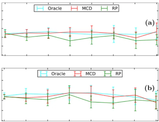
(a) (b)
Figure 5: AUC curves of the methods on datasets generated by a mixture of Gaussian distributions. Observations were equally distributed between the components. γ= 0.4. (a) Mild deviation from normality. m= 4,β= 1.1. RMCD-ℓ2AUC is stable for largep/nratios but is roughly 0.1 below RP and One-Class SVM AUC.
RMCD-RP has the best accuracy. (b) Strong deviation from normality. m = 4, β = 0.7. The different modes are observable in two- or one-dimensional projections of the data. RMCD-ℓ2’s performance is poor compared to OCSVM
p/n 0.1 0.4 0.6 0.8 1.
γ= 20% 1. ±0 1. ±0.005 1. ±0.008 0.99±0.019 0.98±0.027 γ= 30% 1. ±0 0.98±0.023 0.95±0.051 0.90 ±0.104 0.8 ±0.187 γ= 40% 0.65±0.198 0.6 ±0.164 0.59±0.075 0.55 ±0.063 0.58 ±0.084
Table 2: Illustration of the drop of the RMCD-RP-based outlier detection method AUC with the amount of con-taminationγ. Multimodal outliers (p= 100,b= 3,κ(Σ) = 10).
resolution 3mm ×3mm ×3mm. Gaussian smooth-ing at 5mm-FWHM was finally added. T1-weighted MPRAGE [38] anatomical images were acquired with spatial resolution 1mm × 1mm × 1mm, and gray matter probability maps were available for 1986 sub-jects as outputs of the SPM8 ”New Segmentation” algorithm applied to the anatomical images.
5.2. Real data experiments
In a first experiment, we work with five different contrasts images (i.e. linear combination of param-eter images associated with different experimental conditions) that show brain regions implied in simple cognitive tasks (computed on more than 1500 sub-jects):
• an auditory task as opposed to a visual task;
• a left motor task as opposed to a right motor task;
• a right motor task as opposed to a left motor task;
• a computation task as opposed to a sentences reading task;
• an angry faces viewing task;
For outlier detection, we extracted 113 features by computing on each contrast image the average ac-tivation intensity value from 113 regions of inter-est. These regions were given by the Harvard-Oxford cortical and sub-cortical structural atlases2. We re-moved the regions covering more than 1% of the whole brain volume, because the mean signal within such large regions did not summarize well the func-tional signal. We removed the effect of gender, handedness and acquisition center by using a ro-bust regression based on M-estimators [12], using the scikit.statsmodels Python package [31] implementa-tion. We then performed an initial outlier detection
2http://www.cma.mgh.harvard.edu/fsl_atlas.html
at a p-value P < 0.1 family-wise corrected, includ-ing all subjects (n > 1500). With such a small pn value, a statistically controlled outlier detection can be achieved using the MCD estimate. The outlier list obtained from this first outlier detection was then held as a reference labeling for further outlier detec-tion experiments performed on reduced sample sizes, using MCD and all the Regularized MCD estimators. Note that for very small samples, we could not use the MCD-based outlier detection method. The out-lier lists were compared to the reference labeling and ROC curves were constructed. For each sample size, we repeated the detection 10 times with 10 different, randomly selected samples.
We perform a second experiment using the gray matter probability maps available in this database. We use 120 regions of interest defined as 4mm-radius balls centered around locations of highly variable gray matter probability value trough subjects: we used the watershed algorithm [20] to segment the voxel-wise variability map into homogeneous regions, and the signal peak locations of the 120 regions of high-est mean signal were retained as regions of interhigh-est. We limited the number of regions to 120 in order to keep an accurate statistical control of outlier detec-tion with the full dataset. However, the choice and the size of the regions as well as the different type of data used in this second experiment should demon-strate how well regularized covariance-based outlier detection methods generalize to different contexts en-countered in medical imaging. For the sake of com-pleteness, we also tried outlier detection using the Harvard-Oxford atlas regions of interest on the gray matter probability maps.
Figure 6: Results on functional MRI data after removal of the effect of gender, handedness and acquisition cen-ter. AUC curve illustrating the ability of each method to find back a reference labeling from randomly selected sub-samples corresponding to variousp/n ratios. Reference labeling was constructed with the MCD fromn = 1995 observations (p= 113).
5.3. Results
5.3.1. Functional neuroimaging.
Figure 6 shows the outlier detection performance obtained on a dataset constructed from an fMRI contrast reflecting the brain activity related to an-gry faces viewing. The RMCD-RP method’s curve dominates the others methods’ curves forp/n >0.2. RMCD-ℓ2’s accuracy is always above 0.9 while
MCD-based outlier detection breaks down when p/n be-comes large.
Results obtained without removing the effect of gender, handedness and acquisition center are similar to our first results, although the difference between RMCD-RP and RMCD-ℓ2is a bit larger (not shown).
Results obtained with others functional contrasts are similar to those of Figure 6. This suggests that the general structure of observations distribu-tion does not depend on the contrast. Figure 7
shows activity maps (thresholded atP <0.01 family-wise corrected) of out- and inliers subjects in a plot of the first two components of a Principal Compo-nents Analysis performed on the full, outlier-free data set. Outlier observations were projected to the same
low-dimensional space. Outliers found by RMCD-ℓ2-based method stand far from the central
clus-ter, which illustrates the accuracy of the method. State-of-the-art MCD finds only three outliers, miss-ing strongly abnormal observations. It is clear from the figure that some observations would be tagged as abnormal because the global activation pattern devi-ates from the standard ones (e.g. too much activity for subjects (a), (b) and (c)). Yet manual screen-ing may not be sufficient to detect some subtleties in the pattern differences. For instance, the dissimilar-ity between subjects (d) and (e) (both were yet in the RMCD-RP support) is not apparent in the low-dimensional projection. Note that some outliers seem to fall amongst inliers due to an artifact of projection since the original data lie in a 100-dimensional space. Indeed, only 70% of the variance is fit by the first two components.
Figure 8shows the results of a group analysis per-formed on a dataset including 100 subjects drawn from the full data set MCD’s support and the 20 strongest outliers found from the full dataset. The analysis was also performed on the same dataset after outliers removal using the RMCD-ℓ2-based method.
Results of both analyses were compared to a group analysis performed on the whole inliers set (1414 sub-jects). Activation in the left Globus Pallidus was missed in the contaminated set, but was detected af-ter outlier removal. Also, activation in the right oc-cipital cortex was only found from the latter dataset. Although it was obtained from less subjects (resulting in a statistical power loss), the group activation pat-tern for the “cleaned” group better reflects the activ-ity pattern of the whole dataset, showing a stronger effect in every activated regions than the group map obtained from the contaminated set.
5.3.2. Anatomical brain images.
Figure 9gives the outlier detection accuracy of the RMCD-ℓ2, RMCD-RP, MCD and OCSVM methods
on gray matter probability maps. Despite the use of a different imaging modality and ROI selection proce-dure, the relative performance of the methods is very similar to the performance obtained in our experi-ment with functional data. The number of outliers is much smaller in the reference labeling (≃3%). The
Figure 7: Neuroimaging data projection on the space spanned by the two principal components of the full, cleaned dataset. Observations tagged as outliers by the RMCD-RP method are indeed outliers at least along the two first PCA components. MCD-based outlier detection method only finds three outliers and misses strong ones. This figure illustrates the difficulty of manual outlier detection: the deviation from normality can result in unusual patterns that are not easily compared to the others.
(a)(x= 3mm,y=−4mm,z=−25mm) cut. (i) (ii) (iii) (b)(x= 20mm,y = 19mm,z=−5mm) cut.
Figure 8: Illustration of the ben-efit of removing outliers. Group activity map (two-sided test for a null intercept hypothesis β = 0, rejected at P < 0.05 level, family-wise corrected) for the an-gry faces viewing task on(i) a re-duced dataset containing 100 inlier subjects and the 20 strongest out-lier subjects,(ii)the same dataset with outliers removed according to RMCD-ℓ2 method, (iii) the full
dataset with outliers removed ac-cording to RMCD-ℓ2 method. The
results of the second row, obtained after removal of the outliers, are closer to the full dataset group analysis than the results of the first row. This illustrates the adverse consequences of including outliers in group-level inference.
MCD drops faster and breaks down for p/n > 0.5. The variability of all methods but RMCD-RP is much larger, which may be related to the deviation from the Gaussian distribution hypothesis that can be ob-served in the PCA plot given inFigure 9.
Using the Harvard-Oxford atlas’s regions of inter-est mean signal as a descriptive feature of the gray matter images, we obtained similar results, confirm-ing the RMCD-RP’s more accurate performance for outlier detection on real datasets (not shown).
6. Discussion
Different models of outliers. The concept of outlier is ill-defined when dealing with medical data. They can be the result of a acquisition issues as well as poor preprocessing. They can also correspond to a pa-tient or a subject with uncommon characteristics. In general, there is no good generative model that pro-duces realistic outliers, so we use three different mod-els to simulate contaminated neuroimaging datasets, assuming that observations are Gaussian distributed. We also investigate deviations from normality by gen-erating inliers according to a mixture of Gaussian distributions contaminated by variance outliers (see Section 4.1.2). The relative performance of the out-lier detection methods that we compare depends on the statistical characterization of outliers in the sim-ulations. We demonstrated theoretically and empiri-cally that the state-of-the-art method, based on the MCD estimator, breaks down in every model, as soon as the number of dimension approaches the number of observations. Our experiments also demonstrated that under each outlier model, it was possible to find a method that outperforms the RMCD-ℓ1-based
out-lier detection method. Each of the three others meth-ods have pros and cons depending on the outlier type under consideration.
RMCD-ℓ2 detects clusters of outliers and is a good
compromise. If the outliers are grouped in clusters separated from the main cluster of inliers, the only method that achieves a perfect outlier detection is the RMCD-ℓ2 (see 4.2.2). The One-Class SVM was
not adapted to this case because it takes densely-populated regions as being composed by inliers and
so considers the clusters of outliers as being valid ob-servations. RMCD-RP’s accuracy drops if the outlier mode gets closer to main mode and if the contamina-tion rate is high, mainly because the projeccontamina-tion tends to reduce the separation between these clusters [4]. RMCD-ℓ2 can focus on the inliers cluster (i.e. the
biggest one) which is consistent with its definition. Because the RMCD-ℓ2’s accuracy is always close to
the accuracy of the best method for every outlier type and any amount of contamination or inliers’ covari-ance matrix condition number, we recommend to use this method by default because it does not require any parameter tuning, it yields interpretable results, and it is faster to compute than RMCD-ℓ1or
RMCD-RP.
RMCD-RP for non-Gaussian distributed data. As most outlier-detection procedures, the RMCD-RP’s accuracy slightly drops as p/n increases. Yet, ex-cept for extreme cases such as multivariate outliers and large condition number(4.2.3) ormultimodal out-liers and large amount of contamination (4.2.2), the method’s AUC is higher than 0.8, which makes it at-tractive in practice. RMCD-RP was shown to have the best accuracy for non-Gaussian distributed data sets (see4.4) under mild or strong deviation from nor-mality. While the performance of RMCD-ℓ2 breaks
with stronger deviations from normality, RMCD-RP performances dominates with a gain in AUC of 0.2 or more in non-Gaussian settings. In medical imag-ing settimag-ings, RMCD-RP can be considered as useful, due to its robustness to deviations from normality. A procedure for the explicit control of false detections with RMCD-RP is presented inAppendix C.
One-Class SVM works well on unimodal datasets.
One-Class SVM has been shown to have the best accuracy for variance and multivariate outliers, pro-vided the condition number of the inliers covariance matrix is not too large (κ(Σ) ≤ 100, see 4.2.3). Otherwise, the number of support vectors required for spanning the whole inliers space and defining a frontier around has to be very large. This does not correspond to our heuristic to set the ν parameter, which is a lower bound on the number of support vec-tors. The remaining issue is the choice of the
One-(a) (b)
Figure 9: Outlier detection accuracy of the RMCD-ℓ2, RMCD-RP, MCD and OCSVM methods on gray
matter probability maps and representation of the corresponding dataset. (a)The relative performance is very similar to the performance obtained with functional data, although MCD drops faster. RMCD-RP still outperforms with an AUC above 0.95. (b)Projection of the dataset according to the first two components of a PCA decomposition. Outliers (in red) and inliers (in black) of the reference labeling are represented.
Class SVM parameters, especially when the inliers are much more variable in certain directions than in others. We plan to investigate in further work the use of robust covariance estimate to compute a distance to improve the performance of the One-class SVM.
Use of non-parametric tools. Non-parametric out-lier detection tool as the One-Class SVM have a strong potential, provided we can set their param-eters correctly. Indeed, non-parametric methods do not rely on any Gaussian nor symmetry assumption, and should therefore be more sensitive. Using a semi-supervised approach, Mour˜ao-Miranda et al. [19] recently demonstrated the ability of the One-Class SVM to capture the shape of an homogeneous part of the data (i.e. the inliers), which makes outlier detec-tion possible as the distance to the One-Class SVM frontier can be used as a measure of abnormality. Our experiments confirm these findings. However, One-Class SVM is ill-suitable to a medical context as the current heuristics used to tune the parameters pre-vent good statistical control, and its lack of simple decision frontier renders its decisions hard to inter-pret.
Performance on neuroimaging datasets. Functional neuroimaging datasets we used appeared to be non-Gaussian distributed. We showed in subsection 4.4
that using regularized versions of the MCD was still relevant to detect outliers. The RMCD-RP estimator is particularly adapted to that context (seeFigure 5
and Figure 9) since the actual outlier detection is made on projected subspaces that appearmore Gaus-sianthan in the native space. Even on small datasets (p/n >0.2), the new outlier detection methods that we propose can detect outliers that would not be de-tected by hand.
7. Conclusion
We modified the Minimum Covariance Determi-nant (MCD), a robust estimator of location and co-variance part of the state-of-the-art outlier detec-tion framework, in order to make it usable for out-lier detection when the number of observations is small compared to the number of features describ-ing them. Our main contribution is to introduce reg-ularization in the definition of the MCD. We give algorithms to actually compute the regularized
es-timates and we propose a method to set the regu-larization parameters. ℓ2 regularization was shown
to perform generally well in simulations, but ran-dom projections outperform the latter in practice on non-Gaussian, and more importantly, on real neu-roimaging data. Outlier detection using Regularized MCD can be performed in medical image processing before any group study, and was shown to advanta-geously replace widely-used manual screening of the data. Stabilizing group analysis is of broad interest in medical applications, such as pharmaceutic stud-ies. Indeed, patient populations often present large heterogeneities and current studies often rely on an objective assessment of inclusion criteria.
Acknowledgments. This work was supported by a Digiteo DIM-Lsc grant (HiDiNim project, No
2010-42D). The data were acquired within the gen project. JBP was partly funded by the Ima-gen project, which receives research funding from the E.U. Community’s FP6, LSHM-CT-2007-037286. This manuscript reflects only the author’s views and the Community is not liable for any use that may be made of the information contained therein.
Appendix A. ℓ1 regularization (RMCD-ℓ1)
We build a regularized version of the MCD using theℓ1 penaltykAkoff =Pi6=j|ai j|that corresponds to the ℓ1 norm of the off-diagonal coefficients of the
matrixA(note that this is not a matrix norm) in the expression of the penalized negative log-likelihood at step 2 of Algorithm1: ( ˆµℓ1,Σˆℓ1|H) = argmin µ,Σ log|Σ| +1 h X i∈H (xi−µ)TΣ−1(xi−µ) +λkΣ−1k off . (A.1)
We denote the corresponding estimator RMCD-ℓ1.
The solution of this problem is known to have a sparse inverse [34]. This sparsity property is useful for interpretation of the solution in terms of graphical
models. For instance in the functional neuroimaging context, not all brain regions are statistically related to each other [36]. The choice of the regularization parameter λ is particularly important, as the esti-mate is very sensitive to this value. When λ → ∞
this converges to a diagonal matrix. We choose the regularization parameter through an approach using cross-validation (seeAppendix B).
Since no closed form solution exists for the problem (A.1), we use the GLasso algorithm [6], implemented in the scikit-learn package [21].
Appendix B. Alternative strategies to set RMCD’s shrinkage
We report here three strategies that we investi-gated to choose the RMCD-ℓ2 shrinkage parameter:
i) The first strategy is based on likelihood max-imization under the Gaussian distribution model for the inliers. Starting with an initial guess for λ=n p1 Tr( ˆΣ) where ˆΣ is the unbiased empirical covariance matrix of the whole dataset, we iso-late an uncontaminated set of n
2 observations that
correspond to the RMCD’s support. Let λ = δ
n pTr( ˆΣpure), where ˆΣpureis the empirical covariance matrix of the uncontaminated dataset. We choose δ so that it maximizes the ten-fold cross-validated log-likelihood of the uncontaminated dataset. Since we use cross-validation, we refer to theℓ2-regularized
version of the MCD byRMCD-ℓ2(cv). We also used
this strategy for the choice of the RMCD-ℓ1
shrink-age parameter, since the subsequent strategies are not adapted to theℓ1 case.
The two other strategies are based on convex shrinkage, where the estimated covariance matrix
Σlw can be expressed as (1−α) ˆΣ+αpTr( ˆΣ)I. ii)
O. Ledoit and M. Wolf [17] derived a closed formula for the shrinkage coefficientαthat gives the optimal solution in terms of Mean Squared Error (MSE) be-tween the real covariance matrix to be estimated and the shrunk covariance matrix. iii) In a recent work, Chen et al. [1] derived another closed formula that gives a smaller MSE than Ledoit-Wolf formula un-der the assumption that the data are Gaussian dis-tributed. They called it the Oracle Approximating
Shrinkage estimator (OAS). We adapt these results to set the regularization parameter of our MCD ℓ2
-regularized version by taking λ= α⋆
p(1−α⋆)Tr( ˆΣ) for
α⋆ obtained by Ledoit-Wolf and OAS formulas ap-plied to the uncontaminated set, respectively yield-ing estimators that we refer to as RMCD-ℓ2(lw) and
RMCD-ℓ2(oas)estimators.
We did not report the results for RMCD-ℓ2(cv)
-and RMCD-ℓ2(oas)-based outlier detection methods
since they systematically yielded an accuracy lower than or equal to RMCD-ℓ2(lw). This is explained by
the additional hypothesis required by OAS and cross-validation with respect to Ledoit-Wolf approach, and by the suboptimal cross-validation scheme. This find-ing suggests that the cross-validated likelihood may not be optimal as a criterion for choosing the RMCD-ℓ1’s shrinkage parameter and that we do not know
how to set this parameter in practice.
Appendix C. Mahalanobis distance and sta-tistical control
A crucial part of the covariance-based outlier de-tection is the derivation of a threshold on the Maha-lanobis distances that helps performing a statistically controlled decision at the τ type I error maximum level. For any random variableX ∼ N(µ,Σ), it is a well known result thatd2
µ,Σ(X)∼χ2p. Similar re-sult exists for the distribution ofd2
ˆ
µ,Σˆ(X), and [11]
derived a theoretical formula approaching the dis-tribution of the MCD-based Mahalanobis distances d2
ˆ
µh,Σˆh(X) for the observations that were not part of
the MCD’s support (the one within are distributed according to the second result we mentioned). But since the latter approximation only holds for large sample sizes, performing Monte-Carlo simulations re-mains the reference method to assess the distribu-tion of d2
ˆ
µh,Σˆh(X) : considering a n ×p dataset
on which outlier detection has to be performed, the MCD covariance estimate ˆΣh can be used to gen-erate Gaussian distributed data from which a new
ˆ
Σh can be estimated, together with the distribu-tion of the ensuing Mahalanobis distances. Repeat-ing this scheme several times, we obtain a tabulation
(a)
(b)
Figure C.10: Proportion of detected outliers on a clean Gaussian distributed dataset at P < 0.05 un-corrected. (a) κ(Σ) = 1. (b) κ(Σ) = 1000. Type I error rate of RMCD-ℓ2 and RMCD-RP is close to
the nominal value of 0.05 uncorrected chosen in this example.
ˆ
FX : x7→ P(X < x) of the MCD Mahalanobis dis-tance distribution function under the current setting. The same framework can be applied to RMCD-ℓ2, and we adapted it to RMCD-RP in the following
manner:
1. we tabulate the distribution FXk of the
MCD-based Mahalanobis distance undern×ksettings (kis the dimension of the projection subspaces); 2. we takeτ /p as the new accepted error level as the number of random projections is equal top; 3. Taking d∗ = F−1(1−τ /p), define every
obser-vations with Mahalanobis distance greater than d∗ in at least one subspace as outlier.
Despite the approximation made at step 2 of the previous procedure, Figure C.10 shows the propor-tion of type I errors made by the RMCD-RP for a desired theoretical value of τ = 0.05 under various p/nsettings. The final decision is a bit conservative but still relevant.
References
[1] Chen, Y., Wiesel, A., Eldar, Y., Hero, A., 2010. Shrinkage algorithms for MMSE covariance estima-tion. Signal Processing, IEEE Transactions on 58, 5016–5029.
[2] Daszykowski, M., Kaczmarek, K., Heyden, Y.V., Walczak, B., 2007. Robust statistics in data anal-ysis – A review: Basic concepts. Chemometrics and Intelligent Laboratory Systems 85, 203–219. [3] Dave, R., Krishnapuram, R., 1997. Robust
cluster-ing methods: A unified view. Fuzzy Systems, IEEE Transactions on 5, 270–293.
[4] Diaconis, P., Freedman, D., 1984. Asymptotics of graphical projections. The Annals of Statistics 12, 793–815.
[5] Falangola, M., Jensen, J., Babb, J., Hu, C., Castel-lanos, F., Di Martino, A., Ferris, S., Helpern, J., 2008. Age-related non-Gaussian diffusion patterns in the prefrontal brain. Journal of Magnetic Reso-nance Imaging 28, 1345–1350.
[6] Friedman, J., Hastie, T., Tibshirani, R., 2007. Sparse inverse covariance estimation with the lasso. ArXiv e-prints .
[7] Garcia-Escudero, L., Gordaliza, A., 1999. Robust-ness properties of K-Means and trimmed K-Means. Journal of the American Statistical Association 94, 956–969.
[8] Gardner, A., Krieger, A., Vachtsevanos, G., Litt, B., 2006. One-class novelty detection for seizure analysis from intracranial EEG. J. Mach Learn Res 7, 1025– 1044.
[9] Hamilton, W.C., 1970. The revolution in crystallog-raphy. Science 169, 133–141.
[10] Hanley, J.A., McNeil, B.J., 1982. The meaning and use of the area under a receiver operating (ROC) curve characteristic. Radiology 143, 29–36.
[11] Hardin, J., Rocke, D.M., 2005. The distribution of robust distances. Journal of Computational and Graphical Statistics 14, 928–946.
[12] Huber, P.J., 2005. Robust Statistics. John Wiley & Sons, Inc.. chapter 7. p. 149.
[13] Hubert, M., Engelen, S., 2004. Robust PCA and classification in biosciences. Bioinformatics 20, 1728– 1736.
[14] Johnson, W., Lindenstrauss, J., Schechtman, G., 1986. Extensions of Lipschitz maps into Banach spaces. Israel Journal of Mathematics 54, 129–138. [15] Joshi, S., Bowman, I., Toga, A., Van Horn, J., 2011.
Brain pattern analysis of cortical valued distribu-tions. Proc IEEE Int Symp Biomed Imaging , 1117– 1120.
[16] Kherif, F., Flandin, G., Ciuciu, P., Benali, H., Si-mon, O., Poline, J.B., 2002. Model based spatial and temporal similarity measures between series of functional magnetic resonance images. Med Image Comput Comput Assist Interv , 509–516.
[17] Ledoit, O., Wolf, M., 2004. A well-conditioned es-timator for large-dimensional covariance matrices. Journal of Multivariate Analysis 88, 365–411. [18] M´eriaux, S., Roche, A., Thirion, B.,
Dehaene-Lambertz, G., 2006. Robust statistics for nonpara-metric group analysis in fMRI, in: Biomedical Imag-ing: Nano to Macro, 2006. 3rd IEEE International Symposium on, pp. 936–939.
[19] Mouro-Miranda, J., Hardoon, D.R., Hahn, T., Mar-quand, A.F., Williams, S.C., Shawe-Taylor, J., Brammer, M., 2011. Patient classification as an out-lier detection problem: An application of the one-class support vector machine. NeuroImage 58, 793– 804.
[20] Najman, L., Schmitt, M., 1994. Watershed of a con-tinuous function. Signal Processing 38, 99–112. [21] Pedregosa, F., Varoquaux, G., Gramfort, A., Michel,
V., Thirion, B., Grisel, O., Blondel, M., Pretten-hofer, P., Weiss, R., Dubourg, V., Vanderplas, J., Passos, A., Cournapeau, D., Brucher, M., Perrot, M., Duchesnay, ´E., 2011. Scikit-learn: Machine Learning in Python. Journal of Machine Learning Research .
[22] Penny, W.D., Kilner, J., Blankenburg, F., 2007. Ro-bust bayesian general linear models. Neuroimage 36, 661–671.
[23] Pea, D., Prieto, F.J., 2001. Multivariate outlier detection and robust covariance matrix estimation. Technometrics 43, 286–310.
[24] Pinel, P., Dehaene, S., Rivi`ere, D., LeBihan, D., 2001. Modulation of parietal activation by semantic distance in a number comparison task. NeuroImage 14, 1013–1026.
[25] Rousseeuw, P.J., 1984. Least median of squares re-gression. J. Am Stat Ass 79, 871–880.
[26] Rousseeuw, P.J., Leroy, A.M., 2005. Robust Regres-sion and Outlier Detection. John Wiley & Sons, Inc.. chapter 1. pp. 4–5.
[27] Rousseeuw, P.J., Van Driessen, K., 1999. A fast al-gorithm for the minimum covariance determinant es-timator. Technometrics 41, 212–223.
[28] Roux, N.L., Bach, F., 2011. Local component anal-ysis. CoRR abs/1109.0093.
[29] Sch¨olkopf, B., Platt, J.C., Shawe-Taylor, J.C., Smola, A.J., Williamson, R.C., 2001. Estimating the support of a high-dimensional distribution. Neural Comput. 13, 1443–1471.
[30] Schumann, G., Loth, E., Banaschewski, T., Bar-bot, A., Barker, G., B¨uchel, C., Conrod, P., Dal-ley, J., Flor, H., Gallinat, J., Garavan, H., Heinz, A., Itterman, B., Lathrop, M., Mallik, C., Mann, K., Martinot, J.L., Paus, T., Poline, J.B., Robbins, T., Rietschel, M., Reed, L., Smolka, M., Spanagel, R., Speiser, C., Stephens, D., Str¨ohle, A., Struve, M., 2010. The IMAGEN study: Reinforcement-related behaviour in normal brain function and psy-chopathology. Molecular psychiatry 15, 1128–39. [31] Seabold, S., Perktold, J., 2010. Statsmodels:
Econo-metric and statistical modeling with python, in: van der Walt, S., Millman, J. (Eds.), Proceedings of the 9th Python in Science Conference, pp. 57–61. [32] Segata, N., Blanzieri, E., 2009. Fast and scalable local kernel machines. J. Mach Learn Res 11, 1883– 1926.
[33] Shapiro, S.S., Wilk, M.B., 1965. An analysis of variance test for normality (complete samples). Biometrika 52, 591–611.
[34] Tibshirani, R., 1994. Regression shrinkage and se-lection via the lasso. Journal of the Royal Statistical Society, Series B 58, 267–288.
[35] Upadhyaya, A., Rieu, J., Glazier, J., Sawada, Y., 2001. Anomalous diffusion and non-Gaussian veloc-ity distribution of hydra cells in cellular aggregates. Physica A: Statistical Mechanics and its Applica-tions 293, 549–558.
[36] Varoquaux, G., Sadaghiani, S., Pinel, P., Klein-schmidt, A., Poline, J., Thirion, B., 2010. A group model for stable multi-subject ICA on fMRI datasets. NeuroImage 51, 288–299.
[37] Wang, J., Saligrama, V., Casta˜n´on, D.A., 2011. Structural similarity and distance in learning. ArXiv e-prints .
[38] Wetzel, S.G., Johnson, G., Tan, A.G.S., Cha, S., Knopp, E.A., Lee, V.S., Thomasson, D., Rof-sky, N.M., 2002. Three-dimensional, t1-weighted gradient-echo imaging of the brain with a volumet-ric interpolated examination. Amevolumet-rican Journal of Neuroradiology 23, 995–1002.
[39] Woolrich, M., 2008. Robust group analysis using outlier inference. Neuroimage 41, 286–301.
[40] Zweig, M., Campbell, G., 1993. Receiver-operating characteristic (ROC) plots: A fundamental evalua-tion tool in clinical medicine. Clin Chem 39, 561–577.