How to Speed up Optimization? Opposite-Center
Learning and Its Application to Differential Evolution
Hongpei Xu
1, Christiaan D. Erdbrink
2, Valeria V. Krzhizhanovskaya
1,3,41University of Amsterdam, The Netherlands 2Deltares, The Netherlands
3Saint Petersburg Polytechnic University, Russia 4ITMO University, Saint Petersburg, Russia
[email protected], [email protected], [email protected]
Abstract
This paper introduces a new sampling technique called Opposite-Center Learning (OCL) intended for convergence speed-up of meta-heuristic optimization algorithms. It comprises an extension of Opposition-Based Learning (OBL), a simple scheme that manages to boost numerous optimization methods by considering the opposite points of candidate solutions. In contrast to OBL, OCL has a theoretical foundation – the opposite center point is defined as the optimal choice in pair-wise sampling of the search space given a random starting point. A concise analytical background is provided. Computationally the opposite center point is approximated by a lightweight Monte Carlo scheme for arbitrary dimension. Empirical results up to dimension 20 confirm that OCL outperforms OBL and random sampling: the points generated by OCL have shorter expected distances to a uniformly distributed global optimum. To further test its practical performance, OCL is applied to differential evolution (DE). This novel scheme for continuous optimization named Opposite-Center DE (OCDE) employs OCL for population initialization and generation jumping. Numerical experiments on a set of benchmark functions for dimensions 10 and 30 reveal that OCDE on average improves the convergence rates by 38% and 27% compared to the original DE and the Opposition-based DE (ODE), respectively, while remaining fully robust. Most promising are the observations that the accelerations shown by OCDE and OCL increase with problem dimensionality.
Keywords: optimization speed-up; meta-heuristics; Opposite-Center Learning; evolutionary algorithms; continuous optimization; differential evolution; Opposition-Based Learning
1
Introduction
This paper presents an improvement of Opposition-Based Learning (OBL) aimed at boosting the efficiency of meta-heuristic optimization algorithms. The central idea of OBL, introduced by Tizhoosh [4], is to consider not only the candidate solutions generated by a stochastic iteration scheme, but also their 'opposite solutions' found in the opposite regions of the search space. The OBL method has been
Volume 51, 2015, Pages 805–814
ICCS 2015 International Conference On Computational Science
used in many soft computing realms such as Differential Evolution [3], Harmony Search [5], Artificial Neural Network [6] and Particle Swarm Optimization [7]. In optimization problems, the strategy of simultaneously examining a candidate and its opposite solution has the purpose of accelerating the convergence rate towards a globally optimal solution.
To date little effort has been put into developing the theoretical background of OBL [8]. It was proven in [9] that including opposite solutions on average gives shorter expected distances to the global optimum compared to randomly sampled solution pairs. However, the obvious questions whether the opposite point as defined by OBL can be improved or whether it is theoretically the best choice were never posed.
The present study addresses these questions by redefining the opposite point such that the expected distance of the pair consisting of the original candidate and the opposite point to the global optimum is in fact minimized. This results in a new method named Opposite-Center Learning (OCL). This paper provides theoretical and empirical evidence of the positive effects of OCL for continuous optimization problems, since this has been the focus of most OBL applications.
Differential evolution (DE) [2] is a powerful evolutionary algorithm (EA) for solving complex global optimization problems which has abundantly been demonstrated to be efficient and robust and which has been applied to diverse fields such as system identification [12] and antenna design [13]. Among the many proposed improvements to the original DE algorithm is Opposition-based Differential Evolution (ODE) [3], an application of OBL to DE that explores and exploits the opposite points during the DE run. In order to test and showcase the effectiveness of the new Opposite-Center Learning approach in practice, it makes sense to apply it to DE and compare the performance of the resulting algorithm with ODE.
This paper is organized as follows. Section 2 defines the OCL scheme, analyzes it theoretically and gives the computational recipe. In Section 3 a performance comparison between OCL and OBL is presented up to dimension 20. Next, Section 4 shows how OCL can be implemented to solve continuous optimization problems by applying it to DE, thus establishing the new algorithm: Opposite-Center Differential Evolution (OCDE). The experimental results of testing OCDE against ODE and the original DE on a set of benchmark functions are given in Section 5. Finally, Section 6 contains concluding remarks and an outlook on possible future work.
2
Opposite-Center Learning Methodology
2.1
General definition and one-dimensional case
This study deals with solving continuous global optimization problems. It is assumed here that a unique globally optimal solution exists. Let us start by giving the definition of the opposite point as defined by OBL [4].
Definition of opposite point according to OBL: Let ൌ ሺݔଵǡ ݔଶǡ ڮ ǡ ݔሻ א Թ be the starting
point, with ݔא ሾܽǡ ܾሿ ؿ Թǡ ݅ א ሼͳǡ ʹǡ Ǥ Ǥ ǡ ܦሽǡ where D is the problem dimensionality. Then all
coordinates ைǡ of the opposite point ை are defined by
ைǡ ൌ ܽ ܾെ ݔǤ (1) The OBL scheme computes both points and subsequently selects the point with the best fitness value and disposes of the other point. For a minimization problem with a fitness function F, therefore, we compute ሼܨሺሻǡ ܨሺைሻሽ and the corresponding solution (i.e. the starting pointor the
opposite pointை) is returned as output.
The advantage of OBL is derived from the fact that the points generated by OBL have a shorter expected distance towards the global minimum than randomly generated ones. This leads to the question whether the expected distance can be further reduced. This study gives an affirmative answer.
We start by defining an evaluation function that allows analytical assessment of the candidate points.
Definition of evaluation function݃ሺሻ: Let א Թ be a randomly initialized point and௦א
Թ be the global optimum. The evaluation function ݃ሺሻ of candidate point א Թ is defined as
݃ሺሻ ൌ ॱሺሼԡെ ௦ԡǡ ԡ െ ௦ԡሽሻ, (2)
or equivalently as ݃ሺሻ ൌ ሼԡെ ௦ԡǡ ԡ െ ௦ԡሽ ݂ሺ௦ሻ࢙݀Ǥ (3)
Here݂ሺ௦ሻ is the supposed probability distribution function of௦ and “ԡǤ Ǥ Ǥ ԡ” is a suitable
distance metric (in this paper we consider Euclidean and squared distance, but other choices are allowed). This evaluation function measures the expected norm between the optimal point and the point nearest to it. By the logic of this function݃ሺሻ, Rahnamayan et al. [9] proved that OBL performs better than random sampling under the Euclidean norm if there are global optima that are distributed uniformly. Here, the focal point of our efforts is on findingsuch that
ൌ
݃ሺሻ. (4)
Definition of opposite center pointை: Let ൌ ሺݔଵǡ ݔଶǡ ڮ ݔሻ א Թ be the starting point,
with ݔଵǡ ݔଶǡ ڮ ǡ ݔא Թ and let ௦ൌ ሺݔ௦ଵǡ ݔ௦ଶǡ ڮ ݔ௦ሻ be the global optimal point,
withݔ௦ଵǡ ݔ௦ଶǡ ڮ ݔ௦א Թ. Then the opposite center point is defined by
ைൌ
ೞאॻԡ െ ௦ԡ݂ሺ௦ሻ࢙݀,
whereॻ ൌ ሼ௦ǣ ԡെ ௦ԡ ԡ െ ௦ԡሽ. (5)
Applying formula (5) to a one-dimensional problem gives an analytical solution:
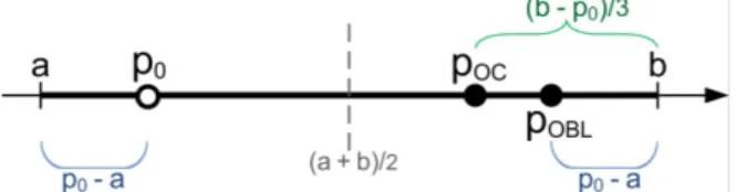
ைൌ ቐ బ ଷ ଶ ଷǡ א ቂܽǡ ା ଶ ቃ బ ଷ ଶ ଷǡ א ቂ ା ଶ ǡ ܾቃ . (6)
To illustrate definitions (1) and (5) and solution (6), Figure 1 sketches the geometric construction of the opposite point in OBL and the opposite center point in OCL for dimension one and݂ሺ௦ሻ
distributed uniformly.
Figure 1: Sketched definition of the opposite center pointࡻin one dimension. The opposition-based point
ࡻࡸand the starting pointare also indicated.
If we consider the supposed global optimum distribution݂ሺ௦ሻ as the density of the search space, the opposite center point can be described as the weighted center of the region where all points have shorter distances to it than to the starting point. Different metrics correspond to different kinds of center. For example, if we take the Euclidean norm, then the geometric median is computed. The
squared distance measure corresponds to the center of mass (centroid). The selection of norm or metric will be discussed in the next subsection.
2.2
Computational scheme for higher dimensions
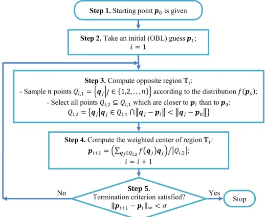
There is no straightforward way of finding the opposite center point deterministically for arbitrary dimension. Therefore an iterative scheme is proposed to approximate the opposite center point in Figure 2.
Figure 2: Flow chart of the Opposite-Center Learning (OCL) scheme.
In Step 4, function݂ሺ௦ሻ is the supposed distribution of the optimum (the objective function). In case there is no information about the distribution, a uniform distribution can be assumed over the search space.
In simple cases (1D or 2D) the Euclidean norm is a suitable choice for the OCL scheme. However, unfortunately the region center for the Euclidean norm (geometric median) is hard to compute in higher dimensions, even when݂ሺ௦ሻ is a uniform distribution. In contrast, the center of mass (centroid), which corresponds to the squared distance, is computationally cheap and also suitable for Riemannian manifolds, where݂ሺ௦ሻ does not have to be uniform. Despite the simplicity of this
metric, though, the computation of the centroid may still be expensive in high dimensional cases. Therefore Step 3 of the scheme (Figure 2) is performed with the Monte Carlo (MC) method to find an approximate centroid.
Step 1. Starting pointisgiven
Step 2. Take an initial (OBL) guessଵ;
݅ ൌ ͳ
Step 3. Compute opposite regionॻ:
- Sample݊ pointsܳǡଵൌ ቄቚ݆ א ሼͳǡʹǡ Ǥ Ǥ ǡ ݊ሽቅ according to the distribution݂ሺ௦ሻ; - Select all points ܳǡଶك ܳǡଵ which are closer to than to:
ܳǡଶൌ ൛หא ܳǡଵځฮെ ฮ ൏ ฮെ ฮൟ
Step 4. Compute the weighted center of regionॻ:
ାଵൌ ቀσೕאொǡమ݂൫൯ቁ หܳൗ ǡଶห;
݅ ൌ ݅ ͳ
Stop Yes
Step 5.
Termination criterion satisfied?
ԡାଵെ ԡஶ൏ ߪ
Experiments shown in Figure 3 indicate that the standard deviation of MC-simulated centroids is
ߪ ൎ ͲǤ͵ ξܰΤ in dimensions 5, 10, 20 and 30, with N the number of MC trials. It is shown that a thousand MC trials generally suffice to attain an error less than 1% (marked by a green dashed line in Fig. 3) in any dimension up to 30.
Figure 3: Monte Carlo experiments used in Step 3 in dimensions 5, 10, 20, 30.
For the termination criterion (Step 5 in Figure 2) we consider that iteration can be stopped if
ԡାଵെ ԡஶ൏ ߪ. The infinity norm stands for the maximum element in the vectorାଵെ . The iterative scheme in Figure 2 produces a series of points that converges to the opposite center point in the limit݅ ՜ λ. Preliminary tests suggest that usually only three to five iterations of the loop in Figure 2 are required to satisfy the termination condition.
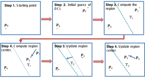
To further explain the OCL scheme, Figure 4 illustrates the main working of the scheme in two dimensions (same steps as in Figure 2).
Figure 4: Illustration of OCL scheme in two dimensions.
Step 1. S tarting point Step 2. Initial guess of
O C L ଵ ॻଵ Ͳ Ͳ ͳ Ͳ Ͳ Ͳ ͳ ʹ ʹ ʹ ॻͳ ॻʹ ॻ ʹ ͵
Step 3. U pdate region Step 4. U pdate region
center
Step 4. C ompute region
center,
Step 3. C ompute the
3
Numerical experiments: sampling
3.1
Verification in one dimension
The OCL scheme of Section 2 is tested by applying it to a simple sampling problem. We compare OCL with OBL and with random sampling using Euclidean distance and squared distance as metrics and assuming a uniform distribution ݂ሺ௦ሻ between 0 and 1. The set-up of this experiment is identical
to that appearing in [9] for OBL: the locations of the optima are successively fixed atሾͲǡ ͲǤͲͳǡ ͲǤͲʹǡ ǥ ǡ ͲǤͻͻǡ ͳሿ and for each location ͳͲସ point pairs are sampled with each scheme.
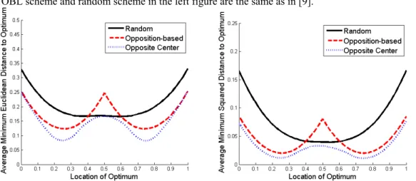
Figure 5 compares the different sampling strategies for two metrics. The value on the vertical axis is the expected distance between the optimum and the closer solution of the pair (see Section 2.1); in the left figure the norm is Euclidean and in the right one the measure is the squared distance. The plots of OBL scheme and random scheme in the left figure are the same as in [9].
Figure 5: Comparison between sampling strategies in one dimension for the Euclidean distance metric (left) and the squared distance metric (right).
From Figure 5 it is clear that the Opposite-Center scheme outperforms the random scheme and the OBL scheme for both metrics. Most significantly, the new scheme yields better results no matter where the optimum is located, except for three points where it is as good as the random scheme (location of optimum at 0.5) and as the OBL scheme (location of optimum near 0 and 1). This means that OCL will beat OBL and random sampling for most non-uniform distributions as well.
3.2
Verification in higher dimensions
Next, the scheme is tested in higher dimensions, again the uniform distribution is assumed and the square of distance is used as metric. For each dimension D, 100D random samples of optima were taken and for each optimum 1000D pairs of points were generated by each scheme.
Figure 6 compares the three different schemes in higher dimensions. The left figure shows average values of evaluation function (3) of generated points. It grows almost linearly with dimension for all three schemes, but the Opposite-Center scheme grows nearly twice as slow as the others. Figure 6, right, shows the minimum difference of evaluation values between OCL and the other two schemes, illustrating the super-linear growth of the advantage of OCL with increasing dimensionality. An important result is that OCL always attains smaller expected nearest squared distances than the other two schemes. Thus, it is computationally verified that the Opposite-Center scheme performs better than the random and opposition-based sampling in dimensions up to 20.
Figure 6: Performancecomparison of Opposite-Center sampling versus Opposition-based sampling and uniformly random sampling up to dimension 20.
4
Application to population-based heuristics
From the definition of OCL it is clear that differentiability and continuity of the objective function are not required. This makes this method very suitable for application to a great variety of heuristic approaches to intractable optimization problems [1]. Opposite-Center Learning can be embedded in population-based stochastic search methods by applying the steps described in Sections 4.1 and 4.2 based on [3].
4.1
Population initialization
By utilizing OCL a better initial population can be created: it is spread more evenly over the search space, so that more information is collected. The following steps describe the procedure:
x Step 1: Generate ݊ൌ ேು
ଶ random pointsሺ݅ ൌ ͳǡʹǡ ǥ ǡ ேು
ଶሻ, where ܰ is the population size. x Step 2: For each random point use the OCL scheme to generate opposite-center points
ைሺ݅ ൌ ͳǡʹǡ ǥ ǡேು ଶሻ.
x Step 3: Assemble all points and ை to create the initial population.
This scheme requires no other property of the fitness function except the prior knowledge of the (approximate) optimum distribution, which may be assumed uniform if it is unknown.
4.2
Generation jumping
The generation jumping scheme takes place after the variation operations in each generation with a probabilityܬܴ (i.e. jumping rate) in the following way:
x Step 1: For ߬ ڄ ܰ points randomly chosen from the population, apply the OCL scheme to generate ߬ ڄ ܰ opposite-center points. Here ߬ א ሺͲǡͳሻ is the exploration rate.
x Step 2: Evaluate fitness of these extra ߬ ڄ ܰ opposite-center points.
x Step 3: Selectܰ points out of the total ሺͳ ߬ሻ ڄ ܰ points. This method does not constrain
the choice for selection scheme.
4.3
Opposite-Center Differential Evolution (OCDE)
Similar to ODE [3], OCL can be applied to differential evolution in two parts: population initialization and generation evolution. It is important to stress that the feasible region where the OCL works changes each generation. Instead of using the original regionሾܽǡ ܾሿ ؿ Թǡ ݅ א ሼͳǡʹǡ ڮ ܦሽ, which is used to form the initial population, the OCL scheme operates in adapted regions
ൣ݉݅݊ǡǡ ݉ܽݔǡ൧ ؿ Թǡ ݅ א ሼͳǡʹǡ ڮ ܦሽ, where ݉݅݊ǡ and݉ܽݔǡ are the minimal and maximal solution values appearing in the population at generation g >1 and in dimension ݅.
5
OCDE experiments
5.1
Set-up
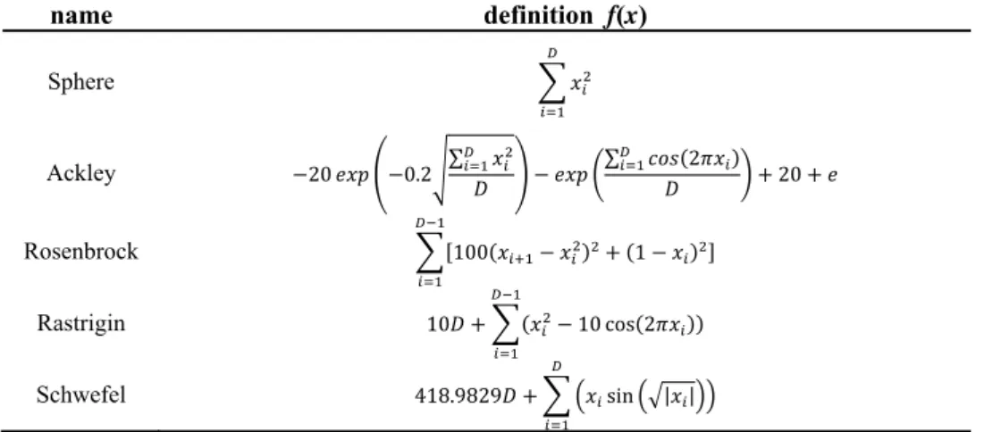
A set of benchmark functions listed in Table 1 is used to test the OCDE algorithm outlined in Section 4. The number of function calls NFC and the success rate are compared in order to investigate convergence speed and effectiveness. The success rate is defined as the percentage of runs in which the value-to-reach VTR is obtained within the set maximum number of function callsܰܨܥ௧. To
compare the converge speeds we calculate the speed-ups of OCDE over ODE and DE as the ratios of
NFC. Model parameters are the same for all three algorithms and all experiments, these are common values used in the references, as listed below.
x Population size,ܰൌ ͳͲ ڄ ܦ [10]
x Differential amplification factor (mutation), ܨ ൌ ͲǤͷ [2]
x Crossover rate, ܥܴ ൌ ͲǤͻ [2]
x Jumping rate constant for ODE, ܬܴைாൌ ͲǤ͵ [3] x Jumping rate constant for OCDE, ܬܴைாൌ ͳȀܦ
x Mutation strategy, DE/rand/1/bin [2]
x Limit of NFC, ܰܨܥ௧ൌ ͳͲ x Value to reach,ܸܴܶ ൌ ͳͲି଼ [11]
In order to maintain a reliable and fair comparison, for all conducted experiments we use an average result of 100 independent runs. Extra fitness evaluations of ODE and OCDE are counted.
name definition f(x) Sphere ݔଶ ୀଵ Ackley െʹͲ ݁ݔ ቌെͲǤʹඨσ ݔ ଶ ୀଵ ܦ ቍ െ ݁ݔ ቆ σୀଵܿݏሺʹߨݔሻ ܦ ቇ ʹͲ ݁ Rosenbrock ሾͳͲͲሺݔାଵെ ݔଶሻଶ ሺͳ െ ݔሻଶሿ ିଵ ୀଵ Rastrigin ͳͲܦ ሺݔଶെ ͳͲ ሺʹߨݔሻሻ ିଵ ୀଵ Schwefel ͶͳͺǤͻͺʹͻܦ ቀݔ ቀඥȁݔȁቁቁ ୀଵ
5.2
Results of the experiments
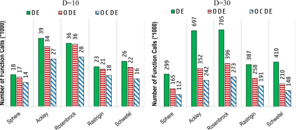
The results are presented in Figure 7 showing the average number of function calls and giving the success rate for the three algorithms on all benchmark functions for dimensions 10 and 30. Equipped with OCL, the convergence speed of OCDE is much higher compared to DE and ODE. In the cases where D=10, OCL accelerates the convergence speed by 38% on average compared to DE and 27% on average compared to ODE. When D=30, OCL performs even better by accelerating the convergence speed by 159% compared to DE and 43% compared to ODE on average. This shows that the idea of Opposite-Center Learning can be used in differential evolution to speed up convergence. Similarly to ODE [3], OCDE performs even better in higher dimensions.
Additionally, the acceleration of convergence does not have a negative influence on the success rate; OCDE achieves a competitive average success rate. Further benchmarking will be needed to draw conclusions about the performance of OCDE on more difficult problems.
D=10 D=30
Figure 7: Performance comparison between DE, ODE and OCDE. Number of function calls for 5 benchmark functions. Left: dimension=10; Right: dimension=30
Benchmark Function
Success Rate Speed-up of OCDE
DE ODE OCDE Compared to DE,
ܰܨܥாΤܰܨܥைா Compared to ODE, ܰܨܥைாΤܰܨܥைா D=10 D=30 D=10 D=30 D=10 D=30 D=10 D=30 D=10 D=30 Sphere 100% 100% 100% 100% 100% 100% 1.318 2.677 1.218 1.480 Ackley 100% 100% 100% 100% 100% 100% 1.437 2.881 1.265 1.455 Rosenbrock 100% 100% 100% 100% 100% 100% 1.276 2.580 1.259 1.449 Rastrigin 99% 93% 95% 93% 99% 96% 1.289 2.023 1.213 1.352 Schwefel 100% 100% 100% 100% 100% 100% 1.633 2.769 1.409 1.423
Table 2: Comparison of success rates of Differential Evolution (DE), Opposition-based Differential Evolution (ODE) and Opposite-Center Differential Evolution (OCDE); and the speed-up of OCDE algorithm over DE and ODE for dimensions D=10 and D=30.
6
Conclusions and future work
The novel Opposite-Center Learning (OCL) scheme presented in this paper improves convergence of population-based search algorithms by smart pair-wise sampling. Given one candidate solution,
18 39 36 23 26 17 34 36 21 22 14 27 28 18 16 Number of Func tion Calls (*10 00 ) D E O D E O C D E 299 697 705 387 410 165 352 396 258 210 112 242 273 191 148 Number of Func tion Calls (*10 00 ) D E O D E O C D E
OCL achieves a minimal expected distance to the global optimum by considering a 'mirror solution' in the opposite region of the search subspace. This technique can be seen as an extension of Opposition-Based Learning (OBL) [4], which has been applied successfully to numerous meta-heuristics.
An iterative computational scheme based on the Monte Carlo method is devised to approximate the opposite center point. Sampling experiments verify that OCL beats OBL up to dimension 20 for an assumed uniform distribution of the optimum.
To tackle continuous optimization tasks, OCL was applied to differential evolution (DE), thus introducing Opposite-Center Differential Evolution (OCDE). The comparison between DE, ODE and OCDE on five common benchmark functions shows that OCDE convergence is accelerated by 38% compared to DE and 27% compared to ODE in 10 dimensions. Remarkably, OCDE achieves even higher acceleration rates in dimension 30 (159% speed-up compared to DE and 43% compared to ODE), which suggests that the beneficial effect of OCL could be most profound in higher dimensional problems. Testing OCDE for dimensions 100 and more will be part of future work. It is expected that OCL will be able to accelerate the convergence of many meta-heuristics and hence can take over the role of OBL.
Ongoing work looks into a number of aspects to further test and improve the method. Analytical work should prove that the optimal point of the evaluation function is in fact equal to the opposite center point and that the given scheme always converges to this point. It could also be examined which metric works best within OCL, how to deal with different distributions of optima and if the sampling strategy can be extended from pairs to multiples. Other future work naturally includes the application of OCL to other evolutionary algorithms such as the Covariance Matrix Adaptation Evolution Strategy (CMA-ES) and the Estimation of Distribution Algorithm (EDA).
Acknowledgements. This work was supported by "5-100-2020" Programme of Russian Federation, Grant 074-U01; and by the Russian Scientific Foundation, project 14-21-00137.
References
[1] Rothlauf, F. (2011). Design of modern heuristics: principles and application. Springer Science & Business Media. [2] Storn, R., Price, K. (1997). Differential evolution–a simple and efficient heuristic for global optimization over continuous
spaces. Journal of global optimization, 11(4), 341-359.
[3] Rahnamayan, S., Tizhoosh, H. R., Salama, M. M. (2008). Opposition-based differential evolution. Evolutionary Computation, IEEE Transactions on, 12(1), 64-79.
[4] Tizhoosh, H. R. (2005, November). Opposition-Based Learning: A New Scheme for Machine Intelligence. In CIMCA/IAWTIC (pp. 695-701).
[5] Qin, A. K., Forbes, F. (2011, July). Dynamic regional harmony search with opposition and local learning. In Proceedings of the 13th annual conference companion on Genetic and evolutionary computation (pp. 53-54). ACM.
[6] Shokri, M., Tizhoosh, H. R., Kamel, M. (2006, July). Opposition-based Q (λ) algorithm. In Neural Networks, 2006. IJCNN'06. International Joint Conference on (pp. 254-261). IEEE.
[7] Dhahri, H., Alimi, A. M. (2010, July). Opposition-based particle swarm optimization for the design of beta basis function neural network. In Neural Networks (IJCNN), The 2010 International Joint Conference on (pp. 1-8). IEEE.
[8] Xu, Q., Wang, L., Wang, N., Hei, X., Zhao, L. (2014). A review of opposition-based learning from 2005 to 2012. Engineering Applications of Artificial Intelligence, 29, 1-12.
[9] Rahnamayan, S., Wang, G. G., Ventresca, M. (2012). An intuitive distance-based explanation of opposition-based sampling. Applied Soft Computing,12(9), 2828-2839.
[10] Brest, J., Greiner, S., Boskovic, B., Mernik, M., Zumer, V. (2006). Self-adapting control parameters in differential evolution: A comparative study on numerical benchmark problems. Evolutionary Computation, IEEE Transactions on, 10(6), 646-657.
[11] Suganthan, P. N., Hansen, N., Liang, J. J., Deb, K., Chen, Y. P., Auger, A., Tiwari, S. (2005). Problem definitions and evaluation criteria for the CEC 2005 special session on real-parameter optimization. KanGAL Report, 2005005.
[12] Erdbrink, C. D., Krzhizhanovskaya, V. V. (2014). Identifying Self-excited Vibrations with Evolutionary Computing. ICCS 2014, Procedia Computer Science, 29, 637-647.
[13] Goudos, S. K., Siakavara, K., Samaras, T., Vafiadis, E. E., Sahalos, J. N. (2011). Self-adaptive differential evolution applied to real-valued antenna and microwave design problems. Antennas and Propagation, IEEE Transactions on,59(4), 1286-1298.