University of Arkansas, Fayetteville
ScholarWorks@UARK
Theses and Dissertations
8-2018
Predicting Changes in Earnings: A Walk Through a
Random Forest
Joshua Hunt
University of Arkansas, Fayetteville
Follow this and additional works at:http://scholarworks.uark.edu/etd
Part of theAccounting Commons
This Dissertation is brought to you for free and open access by ScholarWorks@UARK. It has been accepted for inclusion in Theses and Dissertations by an authorized administrator of ScholarWorks@UARK. For more information, please [email protected], [email protected].
Recommended Citation
Hunt, Joshua, "Predicting Changes in Earnings: A Walk Through a Random Forest" (2018).Theses and Dissertations. 2856. http://scholarworks.uark.edu/etd/2856
Predicting Changes in Earnings: A Walk Through a Random Forest
A dissertation submitted in partial fulfillment of the requirements for the degree of
Doctor of Philosophy in Business Administration with a concentration in Accounting
by
Joshua O’Donnell Sebastian Hunt Louisiana Tech University
Bachelor of Science in Mathematics, 2007 Louisiana Tech University
Master of Arts in Teaching, 2011 University of Arkansas Master of Accountancy, 2013
University of Arkansas
Master of Science in Statistics and Analytics, 2017
August 2018 University of Arkansas
This dissertation is approved for recommendation to the Graduate Council.
____________________________________ Vern Richardson, Ph.D.
Dissertation Director
____________________________________ ____________________________________
James Myers, Ph.D. David Douglass, Ph.D.
Committee Member Committee Member
____________________________________ Cory Cassell, Ph.D.
Abstract
This paper investigates whether the accuracy of models used in accounting research to predict categorical dependent variables (classification) can be improved by using a data analytics approach. This topic is important because accounting research makes extensive use of classification in many different research streams that are likely to benefit from improved accuracy. Specifically, this paper investigates whether the out-of-sample accuracy of models used to predict future changes in earnings can be improved by considering whether the assumptions of the models are likely to be violated and whether alternative techniques have strengths that are likely to make them a better choice for the classification task. I begin my investigation using logistic regression to predict positive changes in earnings using a large set of independent variables. Next, I implement two separate modifications to the standard logistic regression model, stepwise logistic regression and elastic net, and examine whether these modifications improve the accuracy of the classification task. Lastly, I relax the logistic
regression parametric assumption and examine whether random forest, a nonparametric machine learning technique, improves the accuracy of the classification task. I find little difference in the accuracy of the logistic regression-based models; however, I find that random forest has
consistently higher out-of-sample accuracy than the other models. I also find that a hedge portfolio formed on predicted probabilities using random forest earns larger abnormal returns than hedge portfolios formed using the logistic regression-based models. In subsequent analysis, I consider whether the documented improvements exist in an alternative classification setting: financial misstatements. I find that random forest’s out-of-sample area under the receiver operating characteristic (AUC) is significantly higher than the logistic-based models. Taken together, my findings suggest that the accuracy of classification models used in accounting
research can be improved by considering the strengths and weaknesses of different classification models and considering whether machine learning models are appropriate.
Acknowledgements
I would like to thank my mother, Catherine Hunt, who not only taught me how to read, but also instilled in me the importance of education and cultivated my love of learning from an early age.
Table of Contents
Introduction ...1
Algorithms ...10
Logistic Regression ...10
Stepwise Logistic Regression ...14
Elastic Net ...15
Cross-Validation ...18
Random Forest ...19
Data and Methods ...22
Results ...24
Main Analyses ...24
Additional Analyses ...26
Additional Misstatement Analyses ...31
Conclusion ...35
References ...38
Appendices ...43
Tables ...52
1
1. Introduction
The goal of this paper is to show that accounting researchers can improve the accuracy of classification (using models to predict categorical dependent variables) by considering whether the assumptions of a particular classification technique are likely to be violated and whether an alternative classification technique has strengths that are likely to make it a better choice for the classification task. Accounting research makes extensive use of classification in a variety of research streams. One of the most common classification techniques used in accounting research is logistic regression. However, logistic regression is not the only classification technique
available and each technique has its own set of assumptions and its own strengths and
weaknesses. Using a data analytics approach, I investigate whether the out-of-sample accuracy of predicting changes in earnings can be improved by considering limitations found in a logistic regression model and addressing those limitations with alternative classification techniques.
I begin my investigation by predicting positive versus negative changes in earnings for several reasons. First, prior accounting research uses statistical approaches to predict changes in earnings that focus on methods rather than theory, providing an intuitive starting point for my investigation (Ou and Penman 1989a, 1989b; Holthausen and Larcker 1992). While data
analytics has advanced since the time of these papers, the statistical nature of their approach fits in well with a data analytics approach. Data analytics tends to take a more statistical, results-driven approach to prediction tasks relative to traditional accounting research. Second, changes in earnings are a more balanced dataset in regard to the dependent variable relative to many of the other binary dependent variables that accounting literature uses (e.g., the incidence of fraud, misstatements, going concerns, bankruptcy, etc.). Positive earnings changes range from 40% to 60% percent prevalence in a given year for my dataset. Logistic regression can achieve high
2
accuracy in unbalanced datasets but this accuracy may have little meaning because of the nature of the data. For example, in a dataset of 100 observations that only have 5 occurrences of a positive outcome, one can have high accuracy (95 percent for this example) without correctly classifying any of the positive outcomes. Third, focusing on predicting changes in earnings allows me to use a large dataset which, in turn, allows me to use a large set of independent variables. Lastly, changes in earnings are also likely to be of interest to investors and regulators because of their relationship to abnormal returns (Ou and Penman 1989b; Abarbenell and Bushee 1998).
Logistic regression is the first algorithm I investigate because of its prevalent use in accounting literature. Logistic regression uses a maximum likelihood estimator, an iterative process, to find the parameter estimates. Logistic regression has several assumptions.1 First,
logistic regression requires a binary dependent variable. Second, logistic regression requires that the model be correctly specified, meaning that no important variables are excluded from the model and no extraneous variables are included in the model. Third, logistic regression is a parametric classification algorithm, meaning that the log odds of the dependent variable must be linear in the parameters.
I use a large number of independent variables chosen because of their use in prior literature.2
This makes it more likely that extraneous variables are included in the model, violating the second logistic regression assumption. To address this potential problem, I implement stepwise logistic regression, following prior literature (Ou and Penman 1989b; Holthausen and Larcker
1 I only discuss a limited number of the assumptions for logistic regression here. More detail is provided on all of the assumptions in the logistic regression section.
2 Ou and Penman (1989b) begin with 68 independent variables and Holthausen and Larcker (1992) use 60 independent variables. My independent variables are based on these independent variables as well as 11 from Abarbenell and Bushee (1998).
3
1992; Dechow, Ge, Larson, and Sloan 2011). The model begins with all the input variables and each variable is dropped one at a time. The Akaike information criterion (AIC) is used to test whether dropping a variable results in an insignificant change in model fit, and if so, it is permanently deleted. This is repeated until the model only contains variables that change the model fit significantly when dropped.3
While stepwise logistic regression makes it less likely that extraneous variables are included in the model, it has several weaknesses. First, the stepwise procedure performs poorly in the presence of collinear variables (Judd and McClelland 1989). This can be a concern with a large set of independent variables. Second, the resulting coefficients are inflated, which may affect out-of-sample predictions (Tibshirani 1996). Third, the measures of overall fit, z-statistics, and confidence intervals are biased (Pope and Webster 1972; Wilkinson 1979; Whittingham, Stephens, Bradbury, and Freckleton 2001).4
I implement elastic net to address the first two weaknesses of stepwise logistic regression (multicollinearity and inflated coefficients). Elastic net is a logistic regression with added constraints. Elastic net combines Least Absolute Shrinkage and Selection Operator (lasso) and ridge regression constraints. Lasso is an L1 penalty function that selects important variables by shrinking coefficients toward zero (Tibshirani 1996).5 Ridge regression also shrinks coefficients,
but uses an L2 penalty function and does not zero out coefficients (Hoerl and Kennard 1970).6
3 This is an example of backward elimination. Stepwise logistic regression can also use forward elimination or a combination of backward and forward elimination. I use backward elimination because it is similar to what has been used in prior literature (Ou and Penman 1989b; Holthausen and Larcker 1992; Dechow et al. 2011).
4 Coefficients tend to be inflated because the stepwise procedure overfits the model to the data. The procedure attempts to insure only those variables that improve fit are included based on the current dataset and this causes the coefficients to be larger than their true parameter estimates. Similarly, the model fit statistics are inflated. The z-statistics and confidence intervals tend to be incorrectly specified due to degrees of freedom errors and because these statistical tests are classical statistics that do not take into account prior runs of the model.
5 A L1 penalty function penalizes the model for complexity based on the absolute value of the coefficients. 6 A L2 penalty function penalizes the model for complexity based on the sum of the squared coefficients.
4
Lasso performs poorly with collinear variables while ridge regression does not. Elastic net combines the L1 and L2 penalties, essentially performing ridge regression to overcome lasso’s weaknesses and then lasso to eliminate irrelevant variables.
Logistic regression, stepwise logistic regression, and elastic net are all parametric models subject to the assumption that the independent variables are linearly related to the log odds of the dependent variable (the third logistic regression assumption). Given that increasing (decreasing) a particular financial ratio may not equate to a linear increase (decrease) in the log odds of a positive change in earnings, it is not clear that the relationship is linear. To address this potential weakness, I implement random forest, a nonparametric model. The basic idea of random forest was first introduced in 1995 by Ho (1995) and the algorithm now known as random forest was implemented in 2001 by Brieman (2001). Since then it has been used in biomedical research, chemical research, genetic research, and many other fields (Díaz-Uriarte and De Andres 2006; Svetnik, Liaw, Tong, Culberson, Sheridan, and Feuston 2003; Palmer, O’Boyle, Glen, and Mitchell 2007; Bureau, Dupuis, Falls, Lunetta, Hayward, Keith, and Van Eerdewegh 2005).
Random forest is a decision tree-based algorithm that averages multiple decision trees. Decision trees are formed on random samples of the training dataset and random independent variables are used in forming the individual decision trees.7 Many decision trees are formed with
different predictor variables and these trees remain unpruned.8 Each tree is formed on a different
bootstrapped sample of the training data.
These procedures help ensure that the decision trees are not highly correlated and reduce variability. Highly correlated decision trees in the forest would make the estimation less reliable
7 A training data set refers to the in-sample data set used to form estimates to test on the out-of-sample data set. In my setting, I use rolling 5 year windows as training set and test out-of-sample accuracy on the 6th year.
8 Pruning a decision tree refers to removing branches that have little effect on overall accuracy. This helps reduce overfitting.
5
due to the same information being available. Random forest also provides internal measures of variable importance formed from the training set. These measures are constructed by using the out-of-bag error rate from each tree that has been formed in the forest.9
Random forest has several advantages relative to the logistic models. First, this method tends to be an accurate classifier due to its ensemble nature.10 Second, it performs well with a large set
of independent variables, even in the presence of collinear variables, and computes variable importance measures. Third, it is a nonparametric method (i.e., it does not have distributional assumptions). The biggest disadvantage is that random forest tends to over-fit data with noisy classification (i.e. the set of independent variables does a poor job classifying the outcome variable). However, of the four models, random forest is the least restrictive and may improve out-of-sample prediction accuracy.
To predict changes in earnings, I use the change in diluted earnings per share from time t to t+1. I classify those companies that experience a future increase in earnings per share as a positive change and those that do not as a negative change.11 I use independent variables based
primarily on those variables found in Ou and Penman (1989b) and Abarbanell and Bushee (1998). I eliminate variables that are not present for at least 50% of the sample, leaving 71 input variables.12,13 I use these inputs to predict whether earnings changes will be positive.
9 Out-of-bag error is the mean prediction error on the training sample from the bootstrapped subsamples.
10 Ensemble means that a model uses multiple learning algorithms. In this case, random forest uses multiple decision trees.
11 I do not adjust for the trend in earnings as Ou and Penman (1989b) and Houlthausen and Larcker (1992) do in order to preserve the largest possible set of data. All else equal, more data leads to more robust model selection and evaluation.
12 If all variables are required to be present for all of the sample, the sample becomes very small. I examine several cutoffs 40, 50, 60, and 70%. The 50% and lower cutoffs leave the sample and the number of variables large. Several variables are dropped because they are not available in the later years of the sample due to the inclusion of the statement of cash flows. I also examined only taking variables with at least 50% availability for later years 1995, 1999, 2000, 2005, and 2015 to examine the extent of look ahead bias. The variables left in the sample are fairly static, whether examining the entire sample or later years.
6
Following Holthausen and Larcker (1992), I rank the probabilities of changes in earnings in order to have more balanced cutoffs (i.e., I split the samples based on ranked probability cutoffs of 50/50, 60/40, 70/30, 80/20, 90/10, and 95/05). Using this methodology not only balances the top and bottom groups but keeps the number of observations consistent for each model and cutoff. Using raw probability cutoffs yields different sample sizes and unbalanced top and bottom groups.14 I evaluate the out-of-sample accuracy of the classification models and the
abnormal returns generated by trading strategies formed using the predictions from each of the models.
I find that random forest yields better out-of-sample accuracy than the three methods based on logistic regression. Interestingly, the three methods based on logistic regression perform similarly, with elastic net lagging behind logistic regression and stepwise logistic regression. The results suggest that the data may be highly complex because the penalty functions force elastic net to find a simpler model. If logistic regression cannot capture the relation between the independent variables and the outcome, then using an algorithm that forces a simpler relation will almost certainly perform worse.
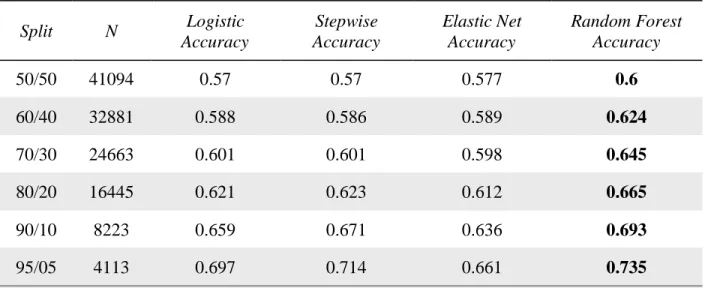
Random forest has higher out-of-sample accuracy for all samples. Specifically, I find that random forest improves out-of-sample classification accuracy over the next closest model by 2.3 for the 50/50 split, 3.5 percent for the 60/40 split, 4.4 percent for the 70/30 split, 4.2 percent for the 80/20 split, 2.2 percent for the 90/10 split, and 2.1 percent for the 95/05 split.
In subsequent tests, I examine the effect that different models have on abnormal returns using the 95/05 split sample. I find that returns are 3 percent larger for random forest than for the next highest return model. This suggests that improving out-of-sample accuracy of the classification
7
of changes in earnings allows investors to earn larger abnormal returns. Because the models use ratios from financial statements, this also provides evidence that financial statements continue to provide information that is not fully reflected in security prices.
I also investigate whether out-of-sample accuracy of classification models can be improved by using a novel validation method. Machine learning algorithms are trained using cross-validation. I use cross-validation in this paper to find the weights for the lasso and ridge regression penalties and to find the number of input variables to use with random forest. Cross-validation allows a researcher to estimate out-of-sample accuracy rates but does not typically take time into account. The main results presented in this paper use traditional K-fold cross-validation (see the methodology section for details). I adapt rolling window, a cross-cross-validation technique used in time-series data, and incorporate it in a pooled cross-sectional data setting. To my knowledge, this is the first paper to implement a cross-validation method that incorporates a time component in pooled cross-sectional data. I find that for a majority of the years in my sample, the out-of-sample accuracy using this cross-validation technique is more similar to the estimated sample accuracy relative to the typical K-fold cross-validation, though out-of-sample accuracy based on ranking probabilities does not improve.
In further analysis, I consider whether the documented improvements exist in an alternative classification setting: financial misstatements. I use the same algorithms as described above: logistic regression, step-wise logistic regression, elastic net, and random forest. I define misstatements as big misstatements if they are disclosed in an 8-K or 8-KA. These reissuance restatements address a material error that requires the reissuance of past financial statements. I drop all other misstatements. I classify those companies that experience big misstatement as a 1 and those that do not as a 0. I use independent variables based primarily on those variables found
8
in Perols, Bowen, and Zimmerman (2017). I eliminate variables that are not present for at least 25% of the sample, leaving 77 input variables. I use random forest to impute the remaining missing values.
I next implement an unsupervised variable reduction technique called variable clustering.15
Variable clustering will find groups or clusters of variables that are highly correlated among themselves and less correlated with variables in other clusters. I then reduce the number of variables by taking those that have the highest correlation with its own cluster and the lowest correlation with other clusters, this reduces the number of inputs to 32.16 I use these inputs to
predict whether big misstatements will occur in a given year.
Because big misstatements are rare, approximately 5% in my sample, I implement three sampling techniques to help with prediction in the presence of an unbalanced dataset. I
implement down-sampling, up-sampling, and SMOTE. Down-sampling balances the data set by taking a random sample of the majority class that is equal size to the less prevalent class. Up-sampling randomly samples the less prevalent class with replacement to match the size of the majority class. SMOTE down samples the majority class and synthesizes new observations for the less prevalent class. I follow Perols et al (2017) and use AUC to assess out-of-sample performance of the misstatement prediction models.
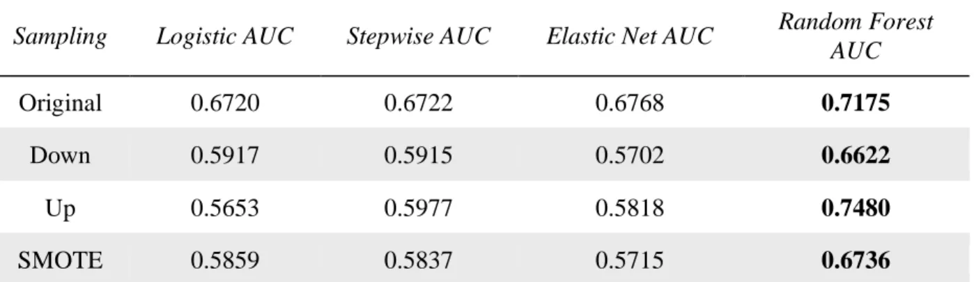
I find that random forest yields a better out-of-sample AUC (0.7462) than the three methods based on logistic regression. Interestingly, the three methods based on logistic regression
perform similarly to each other, with AUC not being statistically different for the original sample at approximately 0.70. The results show that the sampling techniques do not help the logistic
15 Unsupervised refers to an algorithm that does not consider a dependent variable.
16 Results are qualitatively similar without using variable clustering, but computation time is greatly increased. Variable clustering was also implemented with changes in earnings with similar results.
9
models, in fact most of them degrade the fit. Random forest up-sampling performs as good as the original sample random forest. Random forest significantly out-performs the logistic-based models in predicting big misstatements.
I make two main contributions to the literature. First, I provide evidence that the assumptions of the logistic regression may be too restrictive in certain accounting settings and that using a nonparametric machine learning algorithm may improve out-of-sample accuracy.17 Second, I
introduce a novel cross-validation method to the machine learning area that should be of particular interest to accounting researchers due to its panel data nature. I also present a new method to accounting research for assessing the fit of binary predictions called a separation plot (Greenhill 2011). This method allows me to visualize how often high probabilities match actual occurrences and how often low probabilities match nonoccurrences.
While I focus on predicting changes in earnings and financial misstatements, improving the accuracy of classification is likely to benefit other binary outcomes examined in the accounting literature as well. These outcomes include bankruptcy and financial distress (Ohlson 1980; Beaver, McNichols, and Rhie 2005; Campbell, Hilscher, and Szilagyi 2008; Beaver, Correia, and McNichols 2012), goodwill impairments (Francis, Hannah, and Vincent 1996; Hayn and Hughes 2006; Gu and Lev 2011; Li, Shroff, Venkataraman, and Zhang 2011; Li and Sloan 2017), write-offs (Francis et al. 1996), restructuring charges (Francis et al. 1996; Bens and Johnston 2009), initial public offerings (Friedlan 1994; Pagano, Panetta, and Zingales 1998; Teoh, Welch, and Wong 1998; Brau, Francis, and Kohers 2003; Boehmer and Ljungqvist 2003; Brau and Fawcett 2006), seasoned equity offerings (McLaughlin, Safieddine, and Vasudevan 1996; Guo and Mech 2000; Jindra 2000; DeAngelo, DeAngelo, and Stulz 2009; Alti and Sulaeman 2012; Deng,
10
Hrnjic, Ong 2012), and Accounting and Auditing Enforcement Releases (Dechow, Sloan, and Sweeney 1996; Beasley 1996; Beneish 1999; Erickson, Hanlon, and Maydew 2006; Dechow et al. 2011; Feng, Ge, Luo, and Shevlin 2011; Price, Sharp, and Wood 2011; Hribar, Kravet, and Wilson 2013).
2. Algorithms
2.1 Logistic Regression
Logistic regression is the most common classification algorithm in the accounting literature. Logistic regression coefficients are estimated using maximum likelihood estimation, which uses an iterative process to find coefficients that produce a number that corresponds as closely as possible to the observed outcome. Equation 1 is the formula for the maximum likelihood estimation. This method finds β such that the log likelihood is maximized.
log 𝑃(𝑦|𝛽, 𝑥) = ∑𝑚 𝑦𝑖
𝑖=1 log (1+exp(−𝑥1
𝑖𝛽)) + (1 − 𝑦𝑖)log (
exp(−𝑥𝑖𝛽)
1+exp(−𝑥𝑖𝛽)) (1)
Logistic regression does not have the same set of assumptions as ordinary least squares (OLS). First, logistic regression does not assume that error term is normally distributed. Second, it does not assume linearity between the dependent variable and the independent variables. Third, it does not assume homoscedasticity.
Logistic regression is subject to several other assumptions, however. First, the dependent variable must be a categorical variable that represents categories that are mutually exclusive and exhaustive. Second, the model should be properly specified. Related to this assumption, logistic regression performs poorly in the presence of multicollinearity and in the presence of outliers. Third, while linearity between the dependent variable and independent variables is not assumed, linearity between the log odds of the dependent variable and the independent variables is
11
assumed that an adequate number of observations for each category of the dependent variable are available.18
In my first setting, the dependent variable takes a value of one when the change in earnings from year t-1 to year t is positive, and zero otherwise, where earnings are measured as diluted earnings per share. This coding represents two mutually exclusive and exhaustive groups, satisfying the first assumption.19,20
Most techniques assume that the model is correctly specified, but misspecification may be a more serious problem for logistic regression (Mood 2010). Excluding relevant variables results in an omitted variable bias similar to OLS, with the added complication that this bias affects all of the independent variables even if the variable that is omitted is unrelated to the variable of interest (Wooldridge 2002; Mood 2010; Gail, Wieand, and Piantadosi 1984). Including irrelevant variables also creates a problem, depending on the correlation between the irrelevant variables and the other independent variables (Menard 2008). Specifically, the inclusion of irrelevant variables can inflate the standard errors of the irrelevant variables and those of the other independent variables that are correlated with them.
Further, misspecification relates not only to the inclusion/exclusion of variables, but also to the measurement error and multicollinearity of the variables that are included in the final model. The mismeasurement of variables induces bias in coefficient estimates. The measurement error can also come from misclassifications in the dependent variable which can lead to
significant amounts of bias in coefficient estimates (Hausman 2001). Outliers are also a concern.
18 These assumptions are broad and the ordering is not relevant. For more detailed discussions of the assumptions and how to test them, see Hosmer et al (2013) and Menard (2008).
19 Although I am dichotomizing a continuous variable, changes in earnings, I am not interested in the magnitude of the change. That is, I don't predict large changes vs small changes. I predict a positive change in earnings and, in subsequent analyses, I examine whether that prediction is related to abnormal returns.
20 Dichotomizing a continuous dependent variable at the median, mean, or any other cutoff results in a loss of information, which affects the power of the test and increases the false positive rate (Austin and Brunner 2004).
12
Similar to OLS, outliers affect the coefficient estimates and model fit, and can be assessed with traditional methods such as leverage and dfbetas (Menard 2008). Multicollinearity causes inflated standard error estimates and can be assessed using the correlation matrix and variance inflation factors (Menard 2008).
As mentioned above, the third assumption is that the parameters are linear in the logit or log odds of the dependent variable (though linearity between the dependent variable and
independent variables is not assumed). Menard (2008) finds that the failure of this assumption is similar to an omitted variable and will bias coefficients. Similar to OLS, a researcher can include transformations of independent variables in order to assess whether nonlinearities exist or
examine a plot of the logit against the independent variables.21
The fourth assumption is similar to OLS. The error terms are assumed to be uncorrelated. Correlated error terms result when data are related over time and/or space. It may also be related to mismeasurement if the data include non-random measurement error. If this assumption fails, then standard errors tend to be inflated. This assumption is not easily tested and must be
considered when designing the tests. If the data have a time/space component, then error terms are not likely to be independent.
The fifth assumption is that there are an adequate number of observations for each category of the dependent variable. The most extreme form of this potential problem results in zero cells and complete separation. A zero cell occurs whenever the dependent variable is invariant for one or more levels of an independent variable. This will result in a probability of 1 or 0 for an entire group, causing high standard errors and uncertainty related to the coefficient
13
estimate associated with that independent variable (Menard 2008).22 Complete separation refers
to perfectly predicting the dependent variable with a given set of input variables. This can create problems even in less extreme forms, when a given set of input variables predict the dependent variable with extremely high accuracy, but not perfectly (quasi-separation). Both complete and quasi-separation can result in coefficients and standard errors being extremely large.
In this paper, I focus on the assumptions that are likely to affect the accuracy of classification. In particular, the second assumption (model specification) and the third
assumption (linearity between the input variables and the logit) are likely to affect out-of-sample accuracy. While the first assumption can also affect accuracy, the binary dependent variable assumption is generally easily satisfied. Violations of the remaining assumptions can cause problems, such as inflated standard errors and misspecified test statistics but these are unlikely to affect out-of-sample accuracy, the focus of this paper.
Concerns about model specification relate primarily to the inclusion/exclusion of variables, multicollinearity, and outliers. These concerns are likely justified in my setting because of the large number of variables included in the analysis. This makes it likely that
irrelevant variables are included in the model. Multicollinearity is a concern because the majority of the variables are based on common financial ratios that are likely to be related. Outliers are also a common concern when using financial data. The third assumption may not be satisfied because it isn’t clear that forcing every financial ratio to be linearly related to the log odds of a
22 The zero cell assumption only affects dichotomous and nominal variables because continuous and ordered categorical variables have an assumed distributional relationship with the dependent variable and the gaps can be estimated.
14
positive change in earnings is a realistic assumption (i.e., the parametric assumption may be too strong).23 If it is not satisfied, then the effect is similar to an omitted variable bias.
2.2 Stepwise Logistic Regression
In order to address the model specification assumption, I begin with stepwise logistic regression. In my setting I start with a large set of variables, which may suffer from the inclusion of irrelevant variables.24 Backward stepwise logistic regression begins with all of the variables
included and iteratively removes the least helpful predictor (James, Witten, Hastie, and Tibshirani 2013). The Akaike information criterion (AIC) is used to test whether dropping the variable gives an insignificant change in model fit, and if so, the variable is permanently deleted.25 This is repeated until the model only contains variables that change the model fit
significantly when dropped. Hosmer, Lemeshow, and Sturdivant (2013) state that stepwise logistic regression provides an effective data analysis tool because it can provide an effective way to screen a large number of inputs in a new setting.
However, stepwise logistic has several weaknesses. First, the stepwise procedure performs poorly in the presence of multicollinear variables (Judd and McClelland 1989). The deletion of the collinear variables becomes random and it is possible to include noise variables (Hosmer 2013). This can be a concern when using a large set of independent variables. Second, the resulting coefficients are inflated, which may affect out-of-sample predictions (Tibshirani 1996). The coefficients tend to be inflated because the model is overfit to the sample data. This causes the coefficients to be high for that sample and the coefficients are biased high relative to
23 In my setting the parametric assumption is difficult to test because the relation between input variables and target variable may change over time and I examine 45 years.
24 Perols et al. (2017) investigate best subset selection as a method for finding relevant variables. Best subset selection may have statistical issues and overfit the data if the set of variables is large (James et al. 2013). 25 Asymptotically, minimizing the AIC is equivalent to minimizing the error generated from cross-validation estimation (Stone 1977). Other metrics can be used to select variables such as Bayesian information criterion (BIC), pseudo R-squared, Mallows c statistic, etc.
15
the true parameter. Third, the measures of overall fit, z-statistics, and confidence intervals are biased. The test statistics are biased because of multiple testing and because these classical statistics tests were designed for single tests. Fourth, stepwise logistic regression does not guarantee the best model from the subset of total variables because not every combination is tested, and it proceeds with one deletion at a time. Interestingly, the residuals tend to be close to other methods that do iterate through all possible combinations (James et al. 2013).
2.3 Elastic Net
Next, I implement elastic net, a shrinkage method that is based on logistic regression, in order to address the weaknesses of stepwise logistic regression that may affect out-of-sample accuracy (multicollinearity, inflated coefficients, and selecting noise variables). Elastic net still allows the researcher to investigate associations but it should increase out-of-sample accuracy as well. Elastic net is a combination of ridge regression and lasso.26
2.3.1 Ridge Regression
Ridge regression and Lasso are methods that constrain coefficient estimates. Ridge regression is very similar to standard logistic regression, except that the coefficients are
estimated by maximum likelihood with an added constraint, namely the square of the coefficients (James et al. 2013). Equation 2 shows how the estimation of logistic regression is related to ridge regression. Here we minimize the negative log likelihood with the added L2 constraint.
log 𝑃(𝑦|𝛽, 𝑥) = − (∑𝑚 𝑦𝑖 𝑖=1 log (1+exp(−𝑥1 𝑖𝛽)) + (1 − 𝑦𝑖)log ( exp(−𝑥𝑖𝛽) 1+exp(−𝑥𝑖𝛽))) + 𝜑 2∑ 𝛽𝑖 2 𝑘 𝑖=1 (2)
16
The penalized maximum likelihood estimation includes a tuning parameter or shrinking penalty, 𝜑, where higher values increase the penalty and lower values decrease the penalty, all while still finding the maximum likelihood. When the tuning parameter is zero then the model is a standard logistic regression, but as the tuning parameter approaches infinity the coefficients approach zero (James et al. 2013). Because ridge regression shrinks coefficients and coefficient size is dependent on their scale, the inputs must be standardized. I use a standard z-score
standardization, where the independent variables are demeaned and scaled by standard deviation each year.
Standard logistic regression will have low bias but high variance in the presence of many inputs (if the distributional assumption holds). Therefore, a small change in sample may result in a large change in coefficients. Ridge regression has the benefit of reducing the variance of the models produced. That is, if the sample changes, then the model coefficients will change very little. However, ridge regression increases the bias (within an acceptable range) because it shrinks coefficients that have a small effect on the dependent variable close to zero. Ridge regression is also robust to multicollinearity due to the shrinkage penalty. Multicollinearity causes the coefficients to change wildly with small sample changes. The shrinkage function causes coefficients to be more stable while biasing them towards zero. I use cross-validation to identify the best shrinkage parameter (discussed in more detail in section 2.4).
2.3.2 Lasso
The main disadvantage of using ridge regression is that it does not select a subset of variables like stepwise logistic regression.27 To address this, elastic net incorporates lasso in
17
addition to ridge regression. Lasso is very similar to ridge regression with the exception that the penalty added to the maximum likelihood is the absolute value of the coefficients.
log 𝑃(𝑦|𝛽, 𝑥) = − (∑𝑚 𝑦𝑖 𝑖=1 log (1+exp(−𝑥1 𝑖𝛽)) + (1 − 𝑦𝑖)log ( exp(−𝑥𝑖𝛽) 1+exp(−𝑥𝑖𝛽))) + 𝛿 2∑ |𝛽𝑖| 𝑘 𝑖=1 (3)
This is an L1 constraint, where ridge regression uses an L2 constraint. This constraint allows for coefficients to equal zero, effectively selecting the more important variables.28 Lasso contains a
tuning parameter, 𝛿, that controls the amount of shrinkage, similar to the ridge regression. Again, I use cross-validation to identify the best tuning parameter (discussed in more detail in section 2.4).
Although lasso addresses ridge regression’s main disadvantage by reducing the number of variables, it has weaknesses of its own. If the number of variables is greater than the size of the sample (i.e., a large number of variables but a small sample size n), the number of variables that lasso will select is limited by the size of the sample. This is usually not an issue in
accounting research given the typically large data sets used. Lasso also performs poorly in the presence of multicollinearity. If there is a group of multicollinear variables, lasso tends to select one from the group and ignore the rest.
2.3.3 Elastic Net
Elastic net is designed to address many of the weaknesses of ridge regression and lasso. Elastic net uses both the L1 and L2 shrinkage constraints (Zou and Hastie 2005). This allows for the strengths of each of the two methods (ridge regression and Lasso) to overcome the
28 For a detailed discussion of why the L1 penalty results in zeroed out coefficients and the L2 does not, see James et al 2013. The geometric explanation is that the absolute value is not a smooth function and when the optimum coefficient is found it can be at the peak of the function allowing for zero coefficients.
18
weaknesses of the other. The ridge regression penalty addresses multicollinearity and the lasso penalty eliminates nonessential variables.
log 𝑃(𝑦|𝛽, 𝑥) = − (∑𝑚 𝑦𝑖 𝑖=1 log (1+exp(−𝑥1 𝑖𝛽)) + (1 − 𝑦𝑖)log ( exp(−𝑥𝑖𝛽) 1+exp(−𝑥𝑖𝛽))) + 𝜑 2∑ 𝛽𝑖 2 𝑘 𝑖=1 +𝛿2∑𝑘𝑖=1|𝛽𝑖| (4)
Elastic net is subject to the basic assumptions of the logistic regression. The main
weakness is the parametric assumption present in the logistic regression. It also requires that the variables be standardized. The algorithm shrinks coefficients and if the coefficients do not have the same scale then it will perform poorly.
2.4 Cross-Validation
I use cross-validation to identify the two tuning parameters for elastic net (φ and δ). Cross-validation is a resampling technique. Resampling techniques such as cross-validation and bootstrapping are useful when forming an estimate of the implementation error rate and when adjusting tuning parameters.
In order to describe cross-validation, first consider a traditional validation approach that uses a simple random data split of 60-40, where 60% is the training sample or training set and 40% is the out-of-sample or hold out set. The machine learning methods are fit to the training set and their respective fits are assessed on the hold out set. This traditional validation method suffers from two main drawbacks. First, the out of sample error rate can be highly variable because of the random 40 split. If the same methods are performed on a different random 60-40 split, the out of sample error rate can be quite different. Second, the original complete data set is subset to form two smaller data sets. Because statistical methods tend to perform worse on smaller datasets, holding all other factors constant, the estimated error rate tends to overestimate the implementation error rate (James et al. 2013).
19
Cross-validation addresses the two weaknesses of a traditional validation method. K-fold cross-validation divides the training sample into k non-overlapping random samples.29 It then
uses each of the k samples as the hold out sample set and uses the other k-1 samples to fit the model. The hold out sample error rate is averaged over the k hold out sets as tuning parameters are investigated. The final model that is selected is validated using the original complete sample. The advantage to k-fold cross validation is that all of the observations are used for the training and hold out sets, and each observation is used exactly once for the hold out set. The biggest disadvantage is that each statistical method must be run from scratch k times, which increases the computational burden.
I use fold cross-validation for my main tests. Each training data set includes a five-year period. Five random samples are drawn from each training data set and four of the five random samples are used to identify the optimal weights of the elastic net penalty functions. The weights of the penalty functions are randomly generated and tested on the fifth random sample and the accuracy for each random weight is measured. This process is completed four more times using a different random sample each time but using the same initial weights. The test sample accuracy is averaged over each of the five folds and the random weights that produce the highest accuracy are chosen.30 The model is then run on the entire training sample with the chosen
weights. This model is used to form the probability of a positive change in earnings.
2.5 Random Forest
While elastic net addresses several weaknesses of logistic regression, it still assumes that independent variables are linear in the logit, which may be an inaccurate assumption. I address this potential weakness by implementing random forest, a nonparametric model. In order to
29 K-fold cross-validation and cross-validation refer to the same technique.
20
describe random forest, I begin by explaining the components of the model: decision trees and tree bagging.
Decision trees are a set of binary splits. Each split creates an internal node or step that represents a value of one of the input variables. For example, the root node may be the size of a company with the condition that if total assets are greater than 10 million, then split. From this node, it may split again if cash flows are greater than 4 million, and so on. This is a greedy process and is recursive, meaning that it continues to split the data.31 The first split is based on
purity or how well the split separates the data into distinct classes. Every variable and every possible split is considered until the split with the highest purity is found. This happens at each node and continues until a stopping criteria is reached (James et al. 2013).32 New observations
are classified by passing down the tree to a terminal node or leaf.
Decision trees have several strengths. First, because they are nonparametric, there are no distributional assumptions. Second, if the trees are small, then they are easily interpreted. Third, decision trees are robust to outliers and collinear variables. Fourth, they can handle missing data. The main disadvantage is high variability, meaning that a small change in the sample can cause a large change in the final tree (James et al. 2013). This disadvantage leads to the decision tree being a poor classifier. Decision trees tend to overfit the training data and perform poorly out-of-sample.
Tree bagging helps decision trees overcome this weakness. Bagging is a bootstrap aggregation method and is a general purpose tool in machine learning used to reduce model variance. If the prediction method has a lot of variance, then bagging can improve accuracy
31 A greedy algorithm solves for a local optimum with the hope of finding a global optimum. In the case of decision trees, it finds a variable that forms the best split but does not consider future splits.
21
(Breiman 1996). This fits particularly well with decision trees, but can also be applied to other methods. Tree bagging forms decision trees on bootstrapped samples (with replacement) taken from the complete training data set. This allows for different trees to form on each sample. The trees are then averaged (i.e., the classification is accomplished by majority vote).33 Tree bagging
improves classification by reducing the variance, but at the cost of losing the simple tree structure. The bootstrapped samples help ensure that the trees are different, forming a better average. However, tree bagging becomes less effective when the trees are very similar (James et al. 2013).
Random forest addresses this weakness by forming less similar trees. Random forest takes tree bagging one step further by randomly choosing a subset of input variables at each decision tree split. This is done for each tree grown on a bootstrapped sample. For example, if the chosen number of input variables is four, then four variables are chosen at random at each split of the decision tree. The number of variables to be chosen is a tuning parameter. Similar to the other models, I use cross-validation to choose the best tuning parameter for random forest. Specifically, I try a random set of possible numbers limited only by the total number of variables available and choose the number that produces the best cross-validation accuracy.
Random forest tends to be an accurate classifier due to its ensemble nature. Ensemble methods combine the results from different models and can perform better than each of the individual models. Tree bagging is also an ensemble method with the weakness that the combination of multiple trees is moot if the trees are correlated. Because random forest uses random variables at each split, the resulting trees are not highly correlated by construction. Random forest inherits the strengths from decision trees in that it performs well in the presence
33 To classify a new observation the observation is run down every tree in the forest. Each tree has a vote on whether the outcome is positive or not. The forest chooses the outcome that has the most votes.
22
of outliers and highly correlated variables. It also performs well with a very large set of predictor variables and computes variable importance measures. The importance of a variable is estimated using the mean decrease in node impurity (i.e., the important variables aide the most in
classification). Random forest and other tree methods also do not require any variable
transformations, unlike many other machine learning algorithms, including elastic net. Random forest can be applied to data sets with missing data, can be used to find outliers, and can be used to find natural clusters in the data.34
Random forest also has weaknesses. Random forest will over-fit data with noisy
classification (i.e., the set of input variables does a poor job classifying the outcome variable). Its greatest strength can also be a weakness. Random forest is nonparametric. This allows for
complex relationships between the input variables and outcome. Splits are performed on single input variables rather than combinations of input variables and trees can miss relationships, particularly those that logistic regression may capture (Shmueli, Patel, and Bruce 2010).
Logistic regression will outperform nonparametric models, including random forest, if the logistic regression assumptions hold. However, if the parametric assumption fails, then random forest will outperform logistic regression-based models. In sum, random forest is robust to common logistic regression weaknesses and less restrictive in its distributional assumptions and likely to outperform logistic regression-based models in certain settings.
3. Data and Methods
I use independent variables based primarily on variables found in Ou and Penman (1989b) and Abarbanell and Bushee (1998). Ou and Penman (1989b) include levels, changes,
34 For a detailed discussion of what all random forest offers, see https://www.stat.berkeley.edu/~breiman/RandomForests/cc_home.htm
23
and percent changes of financial ratios, but I only include levels and changes.35 The sample
period is between 1965 and 2014 inclusive.36 In order to preserve the sample, all of the Ou and
Penman (1989b) and Abarbenell and Bushee (1998) variables that were not present for at least 50% of the sample are not included. Out of 96 independent variables this left a total of 71 independent variables.37 All of the variables are constructed from Compustat. Each model is run
at the largest available sample that meet the above conditions, which leaves a sample of 101,905 company year observations. The sample consists of December year end firms that have the probabilities available as well as CRSP data, leaving 41,094 company year observations (Ou and Penman 1989a, 1989b; Holthausen and Larcker 1992; Abarbenell and Bushee 1998).38
I use five-year rolling windows as my training sample to predict changes in earnings for the out-of-sample sixth year. For example, my first training sample is 1965-1969 inclusive and I use this sample to predict 1970. The out-of-sample accuracy obtained in 1970 is the metric of interest. Each year the window is rolled forward.39 I use all 71 input variables for each model.
The dependent variable takes a value of one when the change in earnings from year t-1 to year t is positive, and zero otherwise, where earnings are measured as diluted earnings per share. Following Holthausen and Larcker (1992), I rank the probabilities of changes in earnings in order to have more balanced cutoffs, i.e. I rank probabilities for each model and split the sample based on 50/50, 60/40, 70/30, 80/20, 90/10, and 95/05, effectively making percentiles. The 50/50 split halves the dataset and the 95/05 split takes the top 5 percent and bottom five percent of the
35 I only include levels and changes because elastic net requires that the independent variables be standardized and standardizing a percent is nonsensical, but I want each model to contain the same variables. This leads me to include only levels and changes of Ou and Penman (1989) variables.
36 The data is too sparse to begin my sample earlier than 1965. 37 See appendix for variable definitions.
38 I also require companies to have a stock price at the end of year greater than or equal to five dollars.
39 Ou and Penman 1989a, 1989b, and Holthausen and Larcker 1992 use five year blocks. For my time period that means using 1965-1969 inclusive to predict 1970-1974 inclusive and rolling the block forward. In untabulated results every model performs significantly worse with five year blocks relative to what is presented in the paper.
24
probability. Using this methodology not only balances the top and bottom groups, but keeps the number of observations consistent for each model and cutoff. Using raw probability cutoffs yields different sample sizes and unbalanced top and bottom groups.40
4. Results
4.1 Main Analyses
The focus of this section is maximizing out-of-sample accuracy. Table 1 presents the total number of observations per data split and the accuracy for each split and model. Logistic
regression, stepwise logistic regression, and elastic net present nearly identical results for the first 3 splits. Stepwise logistic regression begins to meaningfully outperform logistic regression at the 90/10 split and the 95/05 split (by 1.2 percent and 1.7 percent, respectively). Interestingly, elastic net performs similarly to logistic regression for the first four splits but underperforms logistic regression for the 90/10 split and the 95/05 split (by 2.3 percent and 3.6 percent,
respectively). Remember that elastic net is a logistic regression with two added constraints. Since logistic regression and stepwise logistic regression perform better than elastic net, this may indicate that the data is complex and that using logistic regression is not sufficiently capturing the pattern of the data. If this is the case, then the models are underfitting the data and adding constraints makes the problem worse.
The logistic regression based models are very similar in terms of accuracy for the first three splits. Addressing potential failed assumptions does not improve out-of-sample accuracy within the parametric models. Loosening the distributional assumption with random forest, however, shows an improvement over all of the parametric models (the improvement over logistic regression is as large as 4.4 percent). Random forest performs better (in terms of
25
sample accuracy) for the whole sample in all splits. Because logistic regression will perform better than random forest when the distributional assumption holds, this suggests that the parametric assumption implicit in the logistic regressions may be too strong in this setting. Random forest is able to better capture the more complex relations between the input variables and the output variable.
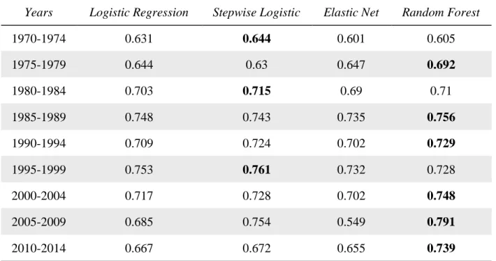
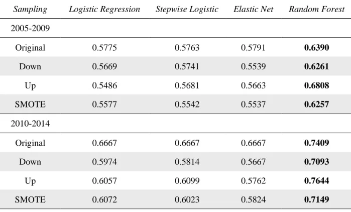
In table 2, I examine out-of-sample accuracy for the 95/05 split in different five-year time periods. I look at five-year time periods beginning with 1970-1974 and ending with 2010-2014, inclusive. Random forest has the highest accuracy for 6 of the 9 time periods. Stepwise logistic regression has the highest accuracy in 1970-1974, 1980-1984, and 1995-1999. Interestingly, the logistic models perform very similarly in all time periods except 2005-2009. This suggests that the differences between the logistic regression-based models in table 1 may be largely due to the 2005-2009 time-period. Stepwise outperforms random forest in 3 time periods (1970-1974, 1980-1984, and 1995-1999), which may indicate that the complexity of the relation between input variables and the outcome variable changes over time. Random forest is consistently the most accurate from 2000 through 2014, the most recent 15 years. This time period includes the dotcom bubble and the financial crisis, which may be why a model that can handle more complex relationships outperforms the other models. The highest accuracy overall accuracy is 79.1 percent during the 2005-2009 time-period.
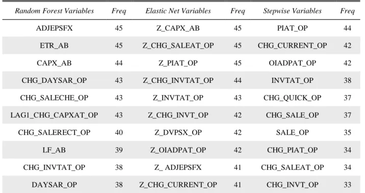
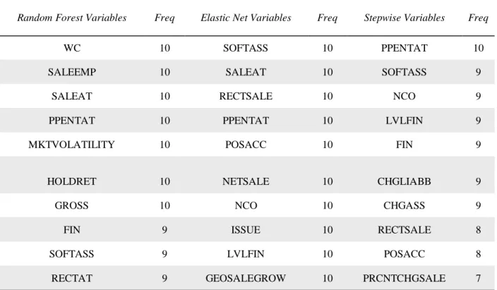
Table 3 investigates which input variables are most important. Table 3 presents the ten input variables chosen most often for stepwise, elastic net, and random forest, and presents the number of years that each respective variable is chosen (45 is the largest possible number of years). Because random forest outperforms the logistic models, it arguably chose best. Random forest chose current year earnings and effective tax rate for every year and capital expenditures
26
44 times. Elastic net chose capital expenditures, change in sales scaled by total assets, and net income scaled by total assets every year. The most frequent variable selected by stepwise logistic regression is net income scaled by total assets. Elastic net has three input variables in common with random forest: capital expenditures, change in inventory scaled by total assets, and current year earnings. Interestingly, stepwise logistic regression did not have any variables in common with random forest.
4.2 Additional Analyses 4.2.1 Abnormal Returns
Though out-of-sample accuracy is the focus of this paper, following prior literature that classifies earnings changes, I also investigate the abnormal returns that can be earned using these methods for the 1970-2014 time period (Ou and Penman 1989b; Holthausen and Larcker 1992; Abarbenell and Bushee 1997). The data corresponds with the accuracy results. Trading begins four months after fiscal year-end (i.e., when current-year results would be widely available for all firms). I present size adjusted abnormal returns held for 12 months. I examine abnormal returns from the 95/05 split for each model because abnormal returns are most likely to be found in the extremes of the distribution.
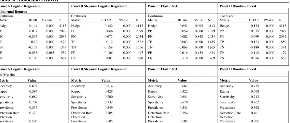
Table 4 presents the abnormal returns results. Panel A presents results using logistic regression, Panel B presents results using stepwise, Panel C presents results using elastic net, and Panel D presents results using random forest. Each panel includes the hedge portfolio return as well as the abnormal returns generated by subsets of the sample: observations predicted positive (PP), those predicted negative (PN), true positives (TP), true negatives (TN), false positives (FP), and false negatives (FN). The number of observations that fall in each of these categories is presented in the fourth column within each respective panel.
27
Table 4 also presents fit metrics in the lower half of each panel. Accuracy is the main metric of interest in this paper but other fit metrics may provide insight into what affects accuracy. Kappa is a measure of how well the classifier performed as compared to how well it would have performed simply by chance. Kappa is not sensitive to class unbalance and can be compared across models. A kappa of 0 corresponds with 50 percent accuracy and a kappa of 100 corresponds with 100 percent accuracy.41 Sensitivity is also called the true positive rate and
recall. Sensitivity measures the proportion of 1's that are correctly classified. Specificity is also called the true negative rate and it measures the proportion of 0's that are correctly classified. Prevalence is a measure of how often 1's occur in the sample. Detection rate is the ratio of true positives to the total number of observations. The detection prevalence is the ratio of predicted positives to the total number of observations.
Logistic regression and stepwise logistic regression perform similarly in terms of the hedge return (14.4 percent and 14.2 percent, respectively) though stepwise outperforms logistic regression for all performance metrics. Elastic net performs the worst with an abnormal return of 5.1 percent. In light of the results presented in table 2, this may be because of poor performance in the 2005-2009 period. The relatively low abnormal return generated using elastic net is likely due to false negatives, which are much larger in number than the other methods. Random forest performs the best both in terms of the hedge return and the performance metrics. The hedge return is 17.4, 3.2 percent higher than logistic regression. It outperforms all other models both for accuracy and kappa. Specificity is particularly large for random forest relative to the other
models at 76.2 percent. It classifies the true negatives at a much higher rate than the other models, with the next highest being stepwise logistic regression at 73.2 percent. The difference
28
in the hedge return appears to be primarily driven by the lower return for predicted negatives (-9.9 percent for random forest versus -6.7 percent for logistic regression).
4.2.2 Incorporating time into Cross-validation
Next, I investigate whether incorporating time into validation in a pooled cross-sectional data setting improves expected accuracy estimation. Because of the time series nature of the data, the k-fold process can be adapted to include a time component. I accomplish this by setting the five training sets to include only the first four years of each five year rolling window and the five hold out sets to include only the fifth year (rolling window cross-validation). This allows me to simulate true implementation conditions during the training phase.
It is an empirical question as to whether rolling window cross-validation will improve the accuracy expectation relative to traditional cross-validation. Traditional cross-validation does not take the order in which the observations occur into account. It takes random samples from the training set to form its k-folds. By forcing the test fold to be the fifth year in the k-fold process, I incorporate a time component in the assessment of the accuracy of the models. I take the
accuracy generated during the rolling window cross-validation and compare it to the out-of-sample accuracy. If the relation between the input variables and the outcome are more or less time invariant, then cross-validation should produce a good estimate of expected accuracy. However, if the relation changes over time, then incorporating time into cross-validation could improve the estimate of expected accuracy. I use random forest to discuss the expected accuracy results and present the difference in expected accuracy produced by both methods.
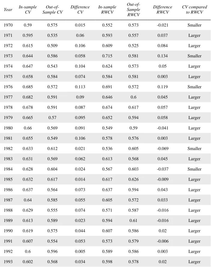
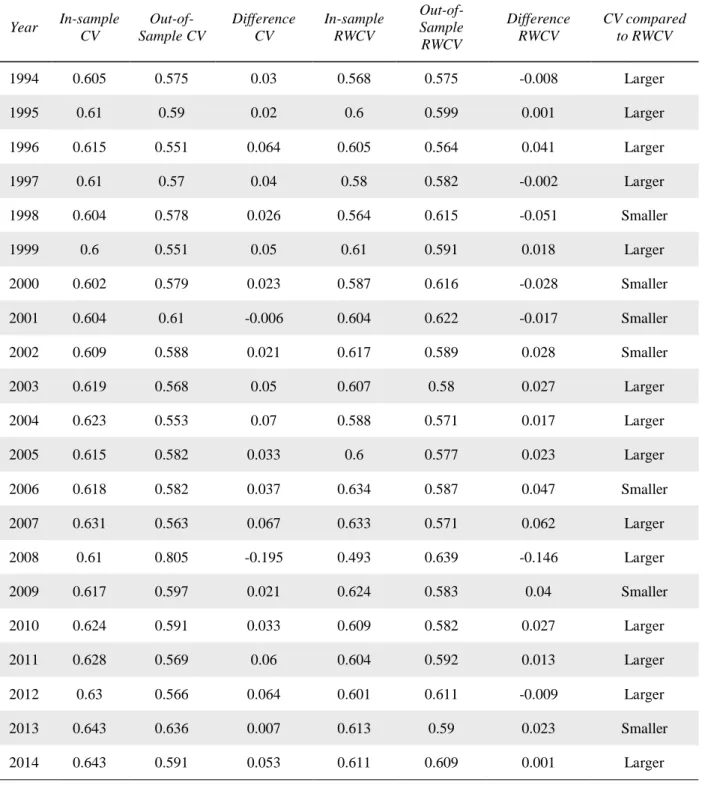
Table 5 presents in-sample accuracy and out-of-sample accuracy for traditional cross-validation (CV) and for rolling window cross-cross-validation (RWCV) for a 50/50 split random forest model. Table 5 also presents the difference between in-sample and out-of-sample accuracy for
29
each of the two validation methods. The last column of table 5 presents the comparison between CV and RWCV. The column compares the absolute value of the in-sample versus out-of-sample difference for CV to the absolute value of the in-sample versus out-of-sample difference for RWCV. The method that produces the smaller absolute difference is the superior model in that year (“Smaller” indicates that CV outperformed RWCV while “Larger” indicates that CV underperformed RWCV). The results show that RWCV outperforms CV in 33 out of 45 years. RWCV likely performs worse when the fifth year of the window is very different from the following year. For example, RWCV performs worse during the dot.com bubble and following the financial crisis in 2009.
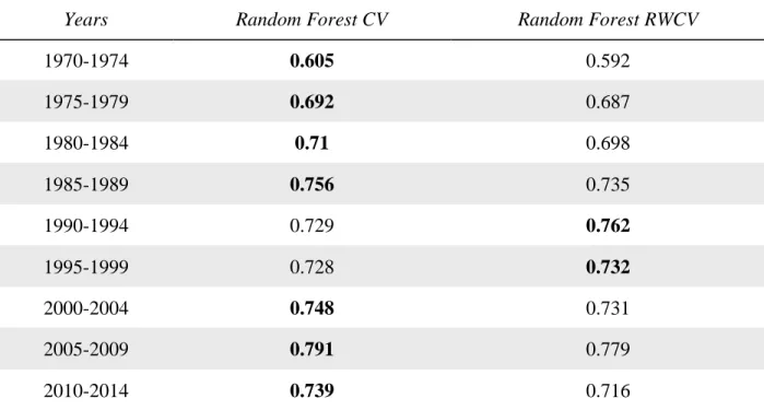
Interestingly, the improved accuracy expectation does not translate into higher out-of-sample accuracy for the 95/05 split. Table 6 presents the accuracy for five year groups for the 95/05 split for random forest. Cross-validation and rolling window cross-validation produce similar out-of-sample accuracy figures. RWCV is higher for only two groups, 1990-1994 and 1995-1999, for the 95/05 split. Rolling window validation outperforms traditional cross-validation in terms of accuracy expectation for the 50/50 split, but not in terms of out-of-sample accuracy at the 95/05 split.
4.2.3 Separation Plots
Next, I present separation plots to assist in analyzing the earnings change data. Separation plots allow users to see the predicted probabilities and the number of instances the actual 1's and 0's occur. Figure 1 shows the separation plot for random forest formed using traditional cross-validation. The gray color represents the 1's and the white color represents the 0's. Moving from left to right along the x-axis should correspond with more occurrences of 1's. The y-axis presents the raw probability of a positive earnings change in year t+1. The black line represents the raw
30
probability associated with each observation ordered from lowest probability to highest probability. An ideal separation plot would be white towards the left of the graph and get increasingly gray towards the right. Figure 1 indicates that most of the raw probabilities are between 40 and 80 percent.
Figure 2 presents the separation plot for random forest formed using RWCV. RWCV appears to tighten the distribution of raw probabilities relative to traditional cross-validation. RWCV also shows more white color towards the left of the graph, suggesting a better fit. This is consistent with the table 5 results.
Figure 3 is a separation plot prepared using ranked probabilities for random forest CV and follows the results presented this paper. The black line represents the rank of raw probability for each observation and is straight by construction. The overall darker right side of figure 3 (relative to figure 1) indicates that ranked probabilities perform better than raw probabilities.
Figure 4 is a separation plot prepared using ranked probabilities for random forest RWCV. Consistent with the results from table 6, comparing figure 3 and figure 4 indicates that CV performs better than RWCV, particularly in the extremes. The overall darker right side of figure 3 (relative to figure 4) indicates that CV performs better (in terms of accuracy) than RWCV.
Greenhill, Ward, and Sacks (2011) describe three main advantages to using separation plots. First, they allow for the actual 1’s and 0’s to be observed. Second, they allow for the range of the predicted probabilities to be visualized. Third, they allow for the relation between
predicted probabilities and actual data to be visualized (i.e., probabilities of 1’s relative to actual 1's). These plots are applicable can be used in any binary classification setting and can be compared across models.
31
4.3 Additional Misstatements Analysis 4.3.1 Data and Methods
Next, I investigate whether the documented improvements exist in an alternative classification setting: financial misstatements. I use independent variables based on variables found in Perols et al (2017). Perols et al. (2017) predict the occurrence of fraud or Accounting and Auditing Enforcement Releases (AAERs) and draw their inputs from other related literature that predicts AAERs (Cecchini, Aytug, Koehler, and Pathak 2010; Dechow et al. 2011; and Perols (2011). The sample period is between 2004 and 2014 inclusive. In order to preserve the sample, all of Perols et al. (2017) variables that are not present for at least 25% of the sample are not included.42 After eliminating variables based on missing observations, I am left with 85
independent variables.43 I follow Perols et al. (2017) and impute missing values with mean and
mode for continuous and dichotomous variables respectively. I run the model at the largest available sample that meet the above conditions, which leaves a sample of 60,873 company year observations.
I use five-year rolling windows as my training sample to predict restatements for the out-of-sample next year. For example, my first training sample is 2000-2004 and I use this sample to predict 2005.44 The out-of-sample AUC obtained in 2005 is the metric of interest. Each year the
window is rolled forward. I follow Perols et al. (2017) in using AUC as my metric of interest. Because the dataset is unbalanced, with restatement occurring approximately 2.26% of the time, using accuracy would be inappropriate. Using my dataset, I could achieve over 97.74% accuracy by guessing no restatement will occur every time, but I would miss every time a restatement did
42 Perols et al. (2017) states that imputation is not advised if more than 25% of the observations are missing per independent variable.
43 See appendix for variable definitions.
32
occur. I define a big restatement as those that are filed in 8-K’s. These reissuance restatements address a material error that requires the reissuance of past financial statements. The dependent variable takes a value of one when there is a current big restatement and zero otherwise.
Because the sample may be unbalanced, I examine three sampling techniques designed to help machine learning algorithms in the presence of rare events: down-sampling, up-sampling, and SMOTE. Theoretically, unbalanced data should not affect the logistic models as long as there are enough observations of the less prevalent class. The maximum likelihood estimation suffers from small-sample bias. This bias is strongly dependent on the number of observations in the less prevalent class. In my setting there are 1,622 cases of big restatements, which should be enough for estimation. However, 2.26% prevalence may be a rare event in the case of random forest.
Each of the sampling methods aim to make the training dataset more balanced in order for the machine learning algorithms to perform better. Unbalanced datasets tend to cause machine learning algorithms to perform well at predicting the majority class, but suffer at predicting the minority class. Down-sampling and up-sampling are essentially opposites of each other. Down-sampling balances the data set by taking a random sample of the majority class that is equal size to the less prevalent class. Up-sampling randomly samples the less prevalent class with replacement to match the size of the majority class. These approaches are less sophisticated than other approaches that are used for balancing datasets, while SMOTE sampling is a more sophisticated sampling method. SMOTE down samples the majority class and synthesizes new observations for the less prevalent class (Chawla, Bowyer, Hall, and Kegelmeyer 2002). SMOTE uses a nearest neighbor approach to synthesize the observations. SMOTE finds observations that are close to one another (nearest neighbors) in the feature space and takes the difference between