Guided Stochastic Gradient Descent Algorithm for inconsistent datasets

(1)

1

Guided Stochastic Gradient Descent Algorithm for Inconsistent Datasets

Abstract

Stochastic Gradient Descent (SGD) Algorithm, despite its simplicity, is considered an effective and default standard optimization algorithm for machine learning classification models such as neural networks and logistic regression. However, SGD’s gradient descent is biased towards the random selection of a data instance. In this paper, it has been termed as data inconsistency. The proposed variation of SGD, Guided Stochastic Gradient Descent (GSGD) Algorithm, tries to overcome this inconsistency in a given dataset through greedy selection of consistent data instances for gradient descent. The empirical test results show the efficacy of the method. Moreover, GSGD has also been incorporated and tested with other popular variations of SGD, such as Adam, Adagrad and Momentum. The guided search with GSGD achieves better convergence and classification accuracy in a limited time budget than its original counterpart of canonical and other variation of SGD. Additionally, it maintains the same efficiency when experimented on medical benchmark datasets with logistic regression for classification.

Keywords: Stochastic Gradient Descent Algorithm, machine learning, classification, logistic regression, neural networks, greedy selection, Guided Stochastic Gradient Descent Algorithm.

1. Introduction

Classification is one of the major techniques in data mining for many applications. Neural networks, logistic regression and support vector machine are some commonly used classification models. Many of these models rely on optimization algorithms for convergence, therefore, accuracy and efficiency of these optimization algorithms have major impact on the quality of classification. Some of the techniques like mathematical Lagrangian method, meta-heuristic algorithms and Gradient Descent Algorithms (GDA) have been employed for solving optimization problems in classification [15, 19, 21, 22]. Optimization problems are

Anuraganand Sharma

School of Computing, Information and Mathematical Sciences The University of the South Pacific, Fiji

[email protected]

(2)

2

generally NP-hard problems where search techniques can have limitation in searching either for a local or the global optimal solutions. GDA generally falls into local optimum solutions for non-convex functions. GDA is an efficient domain data-driven optimization technique, unlike meta-heuristic algorithms that makes it one of the most popular algorithms for machine learning algorithms such as neural networks (NN) and logistic regression [17, 20, 27].

GDA’s two major variants are Stochastic Gradient Descent (SGD) and Batch Gradient Descent (BGD) which will be discussed in detail in Section 2. SGD was derived from BGD to provide an efficient alternative for a gradient descent method. However, the price for efficiency is the untimely random selection of instances which causes high fluctuations in descent or delayed convergence. Additionally, canonical SGD inherits the nature of ‘blind’ search that does not recognize the layout of a given landscape for the optimum descent. This results in slow rate of convergence in some extreme conditions. Many improvements had thus been proposed in order to combat these drawbacks.

1.1Related Work

Qian in [18] has shown the valley-shaped search space has the higher slope for hill gradient compared to the valley that makes the slope direction almost perpendicular to the valley. GDA oscillates near the valley that slows down the convergence. Momentum term [18] is added to reduce the oscillation and improve the convergence. Nesterov Accelerated Gradient (NAG) [29] uses an enhanced momentum terms that also approximates the future positions of the gradient to have even better convergence rate. For sparse data set, Adagrad [7] performs larger updates for infrequent, and smaller updates for frequent parameters. However, in general, its auto updating parameters iteratively becomes ineffective and the learning stops. Adadelta/RMSprop [30] is the improvement of Adagrad by restricting parameters to keep it effective for learning. Hence, the learning rate does not aggressively reduce to minimum in a first few iterations. Adam [12] is another method like Adadelta and RMSprop that computes adaptive learning rates for each parameter. RMSprop, Adadelta and Adam are very similar algorithms that do well in similar circumstances. Adams’ bias-correction helps it to slightly outperform RMSprop towards the end of optimization as gradients become sparser [20].

(3)

3

All these variations had been successfully used with small scale problems in a single machine as traditional formulation of SGD is not suitable for deep learning, particularly in the environment of distributed online learning. Asynchronous SGD has been widely adopted to solve this problem. Moreover, many variations such as RMSprop, Adadelta and Adam show promising results for large scale distributed machine learning algorithms such as deep NN [2, 5, 31, 32]. This paper only focuses on small scale problems where the proposed algorithm, guided SGD (GSGD) works as an add-on to all the variations of SGD. It was shown that GSGD is compatible with all the popular variations of SGD. The algorithm names of the guided versions are prefixed with G such as GRMSprop and GAdam for RMSprop and Adam respectively. However, GSGD is used in this paper to refer to the guided model in general unless otherwise specified. Guided search is not a new approach to improve the search for optimal solutions in optimization algorithms [9, 23], however, the presented approach is a novel idea where guidance is done through consistent data instances.

1.2Problem Statement

The variations of SGD exploit the landscape of the search space to have a faster convergence rate. However, they do not address the poor convergence or low classification accuracy due to the inconsistency present in a dataset. The proposed method is a variation of SGD that overcomes the problem of high inconsistency in a dataset. SGD and its current variations do not have any strategy to filter out the inconsistent data, while the GSGD guides them by selective extraction and exploitation of consistent data instances for gradient descent. Thereby, it improves the convergence quality and classification accuracy. In case of consistent dataset, GSGD would not show any improvement.

The scope of this paper is to analyze the behavior of SGD on inconsistent dataset and provide a better solution using GSGD without compromising the efficiency of SGD. Inconsistency in a dataset is caused by those training examples that result in a net error (or cost) to increase during gradient computation. Mathematical explanation of data inconsistencies is given later on, in the paper. Canonical SGD’s convergence can be improved if the variance in random selection of the instances can be reduced [11, 13]. This can be achieved by temporarily filtering out inconsistent training examples in gradient computation. High variance causes slow convergence with high fluctuations. Therefore, anomaly/outlier detection and removal

(4)

4

techniques should not be applied without appropriate domain analysis [4]. The proposed algorithm does not perform any data cleaning as preprocessing. It is simply a part of training process that tries to distinguish consistent data with inconsistent one to produce better results. A noise is never removed permanently. Moreover, it does not replace the existing outlier detection techniques. The proposed technique provides a competitive alternative for GDA.

The remainder of the paper is organized as follows: Section 2 describes and formalizes various types of GDAs. Section 3 highlights the impact of inconsistent training examples on gradient descent. Section 4 introduces the proposed variation of SGD algorithm known as guided SGD. Section 5 shows comprehensive experiments to compare original variations with guided variations of SGD and Section 6 discusses the outcome of the experiment. Lastly, Section 7 concludes the paper with some suggestions to the future work.

2. Formalization of Gradient Descent Algorithms

GDA is a domain data driven optimization algorithm that has rightly found its niche in machine learning algorithms such as Neural Networks (NN) and logistic regression to optimize the given parameters. GDA iteratively follows the negative gradient of a given activation function in order to move in the direction of descent, to locate the desired minimum. Some commonly used activation functions are sigmoid, tanh and softmax [27]. Sigmoid and softmax have been used for two-class and multi-class classification problems respectively. The optimization problem for linear model (𝑊𝑇_{𝑥 = 0)}_{is formulated as:}

𝑊̂ = argmin W 1 𝑁∑ 𝐸(𝑥𝑛, 𝑦𝑛, 𝑊) 𝑁 𝑛=1

where 𝐸(𝑥𝑛, 𝑦𝑛, 𝑊) is an error or cost function derived from activation function that takes 𝑑

dimensional 𝑁 training examples from (𝑥1, 𝑦1) … (𝑥𝑁, 𝑦𝑁) with 𝑥𝑛 ∈ 𝑅𝑑 and 𝑦𝑛∈ 𝑅, and the

weight vector 𝑊 ∈ 𝑅𝑑_{for two-class classification using logistic regression. For multi-class}

classification with 𝑇 classes, 𝑊 ∈ 𝑅𝑑×𝑇_and_𝑦

𝑛∈ 𝑅𝑇. There are two major variants of gradient

descent based on the manner in which the gradient is calculated, have been described below: 2.1Batch Gradient Descent

Batch Gradient Descent (BGD) is also known as bulk or true gradient descent. In the batch version of gradient descent the weight vector 𝑊(𝑡) is randomly initialized for iteration 𝑡 = 0.

(5)

5

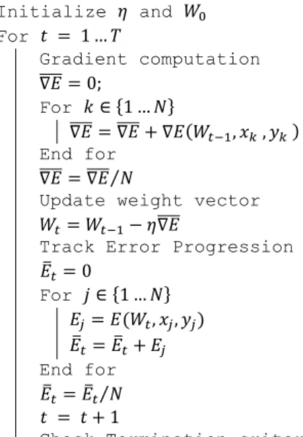
Afterwards, it is iteratively updated such that at each step a short distance is moved in the direction of error’s greatest rate of decrease (steepest descent) for each data instance [3, 10]. However, this does not mean that collectively the steepest descent of error is achieved in every iteration for the entire training examples in every step. The linear models for classification have a perceptron or a set of perceptrons as connectors whose weight vector (or matrix) is to be optimized to get the minimum error. The pseudocode of BGD in logistic regression for classification is given in Fig. 1.

BGD algorithm has only two major steps: average gradient computation and weight update. The algorithm begins with the initialization of learning rate 𝜂, initial weight vector 𝑊0 and

total iterations 𝑇. 𝑊0 is a 0 vector for logistic regression and 𝜂 is generally fixed between 0 – 1

but adaptive learning rates are also being used [16, 28]. The size of training dataset is 𝑁 with 𝑑 dimensions. ∇𝐸(𝑊𝑡, 𝑥𝑖 , 𝑦𝑖 ) is the gradient of error function 𝐸(𝑊𝑡, 𝑥𝑖, 𝑦𝑖) for a given data

instance 𝑥𝑖, its output 𝑦𝑖 and weight vector 𝑊𝑡. The algorithm stops when the termination

criteria is met which is generally the given maximum iterations, or just before the overfitting starts [15]. Initialize 𝜂 and 𝑊0 For 𝑡 = 1 … 𝑇 Gradient computation ∇𝐸 ̅̅̅̅ = 0; For 𝑘 ∈ {1 … 𝑁} ∇𝐸 ̅̅̅̅ = ∇𝐸̅̅̅̅ + ∇𝐸(𝑊𝑡−1, 𝑥𝑘 , 𝑦𝑘 ) End for ∇𝐸 ̅̅̅̅ = ∇𝐸̅̅̅̅ 𝑁⁄

Update weight vector

𝑊𝑡= 𝑊𝑡−1− 𝜂∇𝐸̅̅̅̅

Track Error Progression

𝐸̅𝑡= 0 For 𝑗 ∈ {1 … 𝑁} 𝐸𝑗= 𝐸(𝑊𝑡, 𝑥𝑗, 𝑦𝑗) 𝐸̅𝑡= 𝐸̅𝑡+ 𝐸𝑗 End for 𝐸̅𝑡= 𝐸̅𝑡⁄𝑁 𝑡 = 𝑡 + 1

Check Termination criteria End for

Fig. 1.Pseudocode for Batch Gradient Descent

The batch gradient descent works well if the training data is not too large because computing the gradient term becomes expensive as the data size increases. The time complexity for a single gradient computation is 𝑂(𝑁𝑑) for linear models where 𝑑 is the dimension and 𝑁 is the

(6)

6

size of a given dataset respectively. In case of logistic regression, the overall worst time complexity with 𝑇 iterations would be 𝑂(𝑇(𝑑𝑁 + 𝑁) = 𝑂(𝑇𝑑𝑁), disregarding the early stop due to overlearning.

2.2Stochastic Gradient Descent

Stochastic gradient descent (SGD) addresses the issue of high computational cost by having much faster convergence, in the order of 𝑂(𝑇(𝑑 + 𝑁) only. SGD only differs in how much

data is used to compute the gradient of the objective function. Depending on the amount of data, a trade-off is made between the accuracy in weight update and the time it takes to perform an update [20, 26].

The pseudocode of SGD is given in Fig. 2. SGD also has only two major steps: individual gradient computation and weight update, where it calculates a gradient ∇𝐸(𝑊𝑡, 𝑥𝑖 , 𝑦𝑖 ) of an

instance 𝑖 randomly selected at iteration 𝑡, instead of a true gradient ∇𝐸̅̅̅̅. The definition of all

parameters are same as of BGD algorithm. BGD converges smoothly towards the global minimum for strictly convex error function and possibly to a local minimum for non-convex function. On the other hand, SGD continuously fluctuates to converge, where it helps 𝑊𝑡to

jump to a new and potentially better local minima for non-convex error function [1]. The fluctuations in SGD happens because of high variance in random selection of a single gradient instead of the true gradient of the entire training dataset [11]. The algorithm stops when the termination criteria is met which is again the maximum number of iterations or before the algorithm begins to over learn [15].

Initialize 𝜂 and 𝑊0

For 𝑡 = 1 … 𝑇

For 𝑖 ∈ {1 … 𝑁} selected in a random sequence one at a time.

𝑊𝑡= 𝑊𝑡−1− 𝜂∇𝐸(𝑊𝑡−1, 𝑥𝑖 , 𝑦𝑖 )

Track Error Progression

𝐸̅𝑡= 0 For 𝑗 = 1 … 𝑁 𝐸𝑗= 𝐸(𝑊𝑡, 𝑥𝑗, 𝑦𝑗) 𝐸̅𝑡= 𝐸̅𝑡+ 𝐸𝑗 End for 𝐸̅𝑡= 𝐸̅𝑡⁄𝑁 𝑡 = 𝑡 + 1

Check Termination criteria End for

End for

(7)

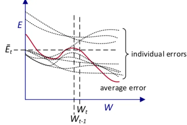
7 W E Wt Ēt Wt-1 average error individual errors

(b) Behavior of individual instances

3. Impact of Data Inconsistency on Gradient Descent

The gradient descent algorithms do not differentiate between consistent and inconsistent training examples. BGD relies on true gradient to nullify the effects of inconsistent data in every iteration. However, determining true gradient in every iteration makes the algorithm very expensive and unsuitable to the applications that require online or deep learning. On the other hand, SGD randomly picks a training example without considering its consistency. That helps in faster convergence and avoidance of many local optimum solutions, however, it may also result in irregular convergence. The analysis of stepwise convergence and effects of inconsistent training example in every iteration in gradient descent is discussed below.

The objective of BGD is to reduce the average error 𝐸̅𝑡 on every iteration 𝑡. At a given weight

vector 𝑊𝑡, on the landscapes of Weights vs Error function, different instances produce

different gradients as illustrated in Fig. 3 (a). The average gradient is not necessarily the steepest gradient at iteration 𝑡. Depending on the sample selection, complexity and noise level of the data, the expectation on every iteration is to have an overall training error ∆𝐸̅𝑡 = 𝐸̅𝑡− 𝐸

̅_𝑡−1≤ 0 which can be given as: ∆𝐸̅𝑡 =

1

𝑁(∆𝐸(𝑊𝑡, 𝑊𝑡−1, 𝑥1, 𝑦1) + ⋯ + ∆𝐸(𝑊𝑡, 𝑊𝑡−1, 𝑥𝑖, 𝑦𝑖) + ⋯ +

∆𝐸(𝑊𝑡, 𝑊𝑡−1, 𝑥𝑁, 𝑦𝑁)) ≤ 0 (1)

where ∆𝐸(𝑊𝑡, 𝑊𝑡−1𝑥𝑖, 𝑦𝑖) = 𝐸(𝑊𝑡, 𝑥𝑖, 𝑦𝑖) − 𝐸(𝑊𝑡−1, 𝑥𝑖, 𝑦𝑖). A rough sketch for this behavior of

individual instances are shown in Fig. 3 (b), where most of the instances have error decreasing at iteration 𝑡 while couple of instances have error increasing.

Fig. 3.Gradients for BGD

(8)

8

The parameters of error functions 𝐸(𝑊_𝑡, 𝑥_𝑗, 𝑦_𝑗), ∆𝐸(𝑊𝑡, 𝑊𝑡−1, 𝑥𝑗, 𝑦𝑗) and ∇𝐸(𝑊𝑡, 𝑥𝑗 , 𝑦𝑗 ) are

replaced with subscripted parameters 𝐸𝑗(𝑊𝑡), ∆𝐸𝑗and∇𝐸𝑗respectively for rest of the paper for

simplicity. From Eq. (1) instances 1,2, … , 𝑖 are considered consistent as their respective errors

are decreasing i.e. {∀ ∆𝐸_𝑗≤ 0 | 𝑗 ≤ 𝑖} and vice-versa for instances 𝑖 + 1, … , 𝑁 where {∀ ∆𝐸_𝑗 > 0 | 𝑗 > 𝑖}. If 𝐸̅𝑡 ∝

1

𝑖∑ ∇𝐸𝑗 𝑖

𝑗=1 and |∑𝑖𝑗=1∆𝐸𝑗| > |∑𝑁𝑗=𝑖+1∆𝐸𝑗| then the error is said to be decreasing

with 𝑊𝑡 = 𝑊𝑡−1− 𝜂∇𝐸̅̅̅̅ for a non-chaotic error function. If the error for training examples {1, … , 𝑖} has the highest Lipschitz constant 𝐿 then the Lipschitz condition for continuity can be

written as:

|∆𝐸𝑗| = |𝐸𝑗(𝑊𝑡) − 𝐸𝑗(𝑊𝑡−1)| ≤ 𝐿|𝑊𝑡− 𝑊𝑡−1|for∀𝑗 ≤ 𝑖 (2)

where 𝐸𝑗(𝑊𝑡) − 𝐸𝑗(𝑊𝑡−1) ≤ 0

The highest Lipschitz constant for ∀𝑗 > 𝑖 has been determined by the summation of Lipschitz

condition from Eq. (2).

∑𝑗=1𝑖 |𝐸𝑗(𝑊𝑡) − 𝐸𝑗(𝑊𝑡−1)|≤ 𝑖𝐿|𝑊𝑡− 𝑊𝑡−1|for∀𝑗 ≤ 𝑖 (3)

Similarly,

|∆𝐸𝑗| = |𝐸𝑗(𝑊𝑡) − 𝐸𝑗(𝑊𝑡−1)| ≤ 𝐿′|𝑊𝑡− 𝑊𝑡−1|for∀𝑗 > 𝑖 (4) ∑𝑗=𝑖+1𝑁 |𝐸𝑗(𝑊𝑡) − 𝐸𝑗(𝑊𝑡−1)|≤ (𝑁 − 𝑖)𝐿′|𝑊𝑡− 𝑊𝑡−1| (5)

where 𝐿′ is the highest Lipschitz constant for ∀𝑗 > 𝑖 and 𝐸𝑗(𝑊𝑡) − 𝐸𝑗(𝑊𝑡−1) > 0. To have

overall descending (or same) error in an iteration 𝑡, the following condition must hold:

(𝑁 − 𝑖)𝐿′_|𝑊

𝑡− 𝑊𝑡−1| ≤ 𝑖𝐿|𝑊𝑡− 𝑊𝑡−1| ∴ 𝐿′≤ 𝑖

𝑁−𝑖𝐿 (6)

In an ideal case, the landscape of training data behaves consistently with every instance, i.e. 𝑖 = 𝑁. So, any small positive value of 𝐿 (𝐿 > 0) would ensure error decreases in every next

iteration until convergence is almost complete. Training examples’ high inconsistency can be tolerated with the true gradient as long as Eq. (6) is true.

(9)

9

SGD does not use true gradient but rather picks up an example randomly. The increase or decrease in error value depends on the presence of inconsistent examples in a given iteration. The error value is determined by the same principles as discussed above from Eq. (1) to Eq. (6); where only the true gradient 𝐸̅𝑡 is replaced by an individual gradient ∇𝐸𝑘, where 𝑘 ∈ {1,2, … , 𝑁}. ∇𝐸𝑘 can be directly proportional to either

1 𝑁∑ ∇𝐸𝑗 𝑖 𝑗=1 or 1 𝑁∑ ∇𝐸𝑗 𝑁 𝑗=𝑖+1 which makes

the error descend or ascend respectively. Generally, for consistent data 𝑖 ≫ (𝑁 − 𝑖); descent

happens more often over the iterations, and of course with a better convergence rate. More specifically, for |∑𝑖𝑗=1∆𝐸𝑗(𝑊𝑡)| > |∑𝑁𝑗=𝑖+1∆𝐸𝑗(𝑊𝑡)| the error 𝐸̅𝑡 decreases if

∇𝐸𝑘 ‖∇𝐸𝑘‖∝ 1 𝑖∑ ∇𝐸𝑗 ‖∇𝐸𝑗‖ 𝑖 𝑗=1

where 𝑘 ≤ 𝑖; otherwise the error increases in a normal circumstances when some data

instances are not chaotic in nature. Using Lipschitz condition for continuity if descend happens only in 𝑡’ iterations out of total 𝑇 iterations then following Eq. (2) and Eq. (4), the

equation for the net descend after 𝑇 iterations would be:

∑𝑡 ∑𝑖(𝑡)𝑗=1|𝐸𝑗(𝑊𝑡) − 𝐸𝑗(𝑊𝑡−1)| ′

𝑡=1 ≤ 𝐿𝑁𝑡′|𝑊𝑡− 𝑊𝑡−1| for net gradient descent

∑𝑇𝑡=𝑡′₊₁∑𝑗=𝑖(𝑡)+1𝑁 |𝐸𝑗(𝑊𝑡) − 𝐸𝑗(𝑊𝑡−1)| ≤ 𝐿′𝑁(𝑇 − 𝑡′)|𝑊𝑡− 𝑊𝑡−1|for net gradient ascent ∴ 𝐿′≤_(𝑇−𝑡𝑡′𝐿_′₎for𝑡′_{< 𝑇}

(7)

Thus, net descent in SGD happens after 𝑇 iterations when Eq. (7) holds true. Otherwise, the algorithm will diverge for the given iterations. In comparison with BGD, gradient descent does not happen in every iteration, however, some fluctuations are seen while the algorithm runs. Convergence for consistent data is smoother compared to inconsistent data. This shows the importance of consistent examples in gradient descent which is the primary focus of this paper.

One issue with SGD is its high variance caused by the random selection of gradient instead of average gradient [11]. Therefore, one logic variation of canonical SGD is the combination of BGD with SGD known as min-batch gradient descent that reduces the variance to some extent and still manages better convergence rate. However, most recent SGD variations discussed in introduction section has transpired that neither decreasing step-sizes nor mini-batching are necessary to resolve the non-vanishing variance issue inherent in the canonical SGD methods [13, 25].

(10)

10

4. Guided Stochastic Gradient Descent Algorithm

After describing BGD and SGD it is evident that high data inconsistency plays a major role in the degree of error descent per iteration and convergence. The proposed algorithm is named as guided stochastic gradient descent (GSGD) algorithm that realizes the importance of inconsistency in a dataset and tries to improve the convergence by separating consistent and inconsistent data instances to some extent. GSGD hides inconsistent data for “a while” in an anticipation that they will become consistent after few iterations. In addition to individual gradient computation and the weight update, GSGD selects consistent instances gradually and does the refinement of the weight update.

Inconsistent data instances are simply the data instances within the neighborhood of instance 𝑗; which individually performs better, while the average error value 𝐸̅𝑡 performs

worse than the average error of the previous iteration 𝐸̅𝑡−1, and vice-versa. The pseudocode of

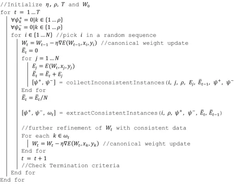
the algorithm is given in Fig. 4 and Fig. 5. The definition of variables used in the GSGD algorithm are same as in SGD and BGD unless otherwise specified. The algorithm begins by initializing weight vector (𝑊0), learning rate (𝜂), total iterations (𝑇) and neighborhood size (𝜌).

Neighborhood allocation allows GSGD to run through 𝜌 training examples recursively before

further refinement of 𝑊 is done with the consistent data. Consistent data is selected from 𝜌

training examples at a time. Each data instance 𝑥_𝑖 with label 𝑦_𝑖 is randomly selected to update the weight vector (𝑊𝑡) at iteration 𝑡 like SGD. The neighborhood of an instance 𝑘 is kept in

sets 𝜓+ and 𝜓− where they track inconsistent instances. After collecting the data about

inconsistency for 𝜌 iterations, only consistent instances are extracted and kept in 𝜓+ and 𝜓−.

𝜓_𝑘+ in the pseudocode refers to 𝑘𝑡ℎ element of either𝜓+ or𝜓−, i.e., {𝜓_𝑘+∈ 𝜓+|𝑘 ∈ {1 … 𝜌}}

and {𝜓_𝑘−∈ 𝜓−|𝑘 ∈ {1 … 𝜌}}. Lastly, 𝑊𝑡 is further updated with consistent instances 𝜔𝑡.

Its flowchart is given in Fig. 6 where the algorithm starts with a random selection of a data instance whose gradient is computed to update the weight vector. After 𝜌 iterations, weight vector is further refined with consistent neighboring data instances. 𝜌 is also the neighborhood size which is generally assigned to a constant value 10.

(11)

11

//Initialize 𝜂, 𝜌, 𝑇 and 𝑊0 for 𝑡 = 1 … 𝑇

∀𝜓𝑘+= 0|𝑘 ∈ {1 … 𝜌}

∀𝜓𝑘−= 0|𝑘 ∈ {1 … 𝜌}

for 𝑖 ∈ {1 … 𝑁} //pick 𝑖 in a random sequence

𝑊𝑡= 𝑊𝑡−1− 𝜂∇𝐸(𝑊𝑡−1, 𝑥𝑖, 𝑦𝑖) //canonical weight update

𝐸̅𝑡= 0 for 𝑗 = 1 … 𝑁 𝐸𝑗= 𝐸(𝑊𝑡, 𝑥𝑗, 𝑦𝑗) 𝐸̅𝑡= 𝐸̅𝑡+ 𝐸𝑗 [𝜓+_{, 𝜓}−_]_{= collectInconsistentInstances(}_{𝑖, 𝑗, 𝜌, 𝐸} 𝑗, 𝐸̅𝑡−1, 𝜓+, 𝜓−) End for 𝐸̅𝑡= 𝐸̅𝑡⁄𝑁 [𝜓+_{, 𝜓}−_{, 𝜔} 𝑡] = extractConsistentInstances(𝑖, 𝜌, 𝜓+, 𝜓−, 𝐸̅𝑡, 𝐸̅𝑡−1) //further refinement of 𝑊𝑡 with consistent data

For each 𝑘 ∈ 𝜔𝑡

𝑊𝑡= 𝑊𝑡− 𝜂∇𝐸(𝑊𝑡, 𝑥𝑘, 𝑦𝑘) //canonical weight update End for

𝑡 = 𝑡 + 1

//Check Termination criteria End for

End for

Fig. 4.Pseudocode for Guided Stochastic Gradient Algorithm [𝜓+_{, 𝜓}−_]_{= collectInconsistentInstances(}_{𝑖, 𝑗,} _{𝜌, 𝐸}

𝑗, 𝐸̅𝑡−1, 𝜓+, 𝜓−) //Determine inconsistent data instances

if ⌊(𝑗 + 𝜌 − 1) 𝜌⁄ ⌋ == ⌊(𝑖 + 𝜌 − 1) 𝜌⁄ ⌋ 𝑘 = 𝑗 − 𝜌⌊(𝑗 + 𝜌 − 1) 𝜌⁄ − 1⌋ if 𝐸𝑗− 𝐸̅𝑡−1> 0 𝜓𝑘+= 𝜓𝑘++ (𝐸𝑗− 𝐸̅𝑡−1) else 𝜓𝑘−= 𝜓𝑘−− (𝐸𝑗− 𝐸̅𝑡−1) End if End if End

Fig. 5.Subroutines for Guided Stochastic Gradient Algorithm

[𝜓+_{, 𝜓}−_{, 𝜔}

𝑡] = extractConsistentInstances(𝑖, 𝜌, 𝜓+, 𝜓−, 𝐸̅𝑡, 𝐸̅𝑡−1)

𝜔𝑡= ∅

Extract consistent data points with respect to 𝑥𝑖 if 𝑚𝑜𝑑(𝑖, 𝜌) == 0

if 𝐸̅𝑡< 𝐸̅𝑡−1;

𝜓+= 𝑠𝑜𝑟𝑡(𝜓+, "Descend");

𝜔𝑡= {𝑘|𝜓𝑘+∈ 𝜓+⋀ 𝜓𝑘+= 0} //get indices with no noise else

𝜓−_{= 𝑠𝑜𝑟𝑡(𝜓}−_{, "Descend");}

𝜔𝑡= {𝑘|𝜓𝑘−∈ 𝜓−⋀ 𝜓𝑘−= 0} //get indices with no noise End if

∀𝜓𝑘+= 0|𝑘 ∈ {1 … 𝜌}

∀𝜓𝑘−= 0|𝑘 ∈ {1 … 𝜌} End if

(12)

12

Fig. 6.Flowchart of Guided Stochastic Gradient Algorithm

The worst time complexity of GSGD is same as SGD even with the addition of sorting and further refinement of the weight vector. Sorting (with quick sort) and further refinement have worst time complexity of 𝜌2_{and 𝑑𝜌 respectively. Hence, overall the worst time complexity of}

GSGD is 𝑂(𝑇(𝑑 + 𝑁 + 𝜌2_{+ 𝑑𝜌)) = 𝑂(𝑇(𝑑 + 𝑁)}_{which is same as SGD because}_{𝜌 ≪ 𝑁}_{is a}

constant term. It is also interesting to note that GSGD is same as SGD for the first 𝜌 iterations. Therefore, it is very important to choose an appropriate value of 𝜌as its very large value will simply make the algorithm original SGD. As such, more analysis has been done on it in Section 5.

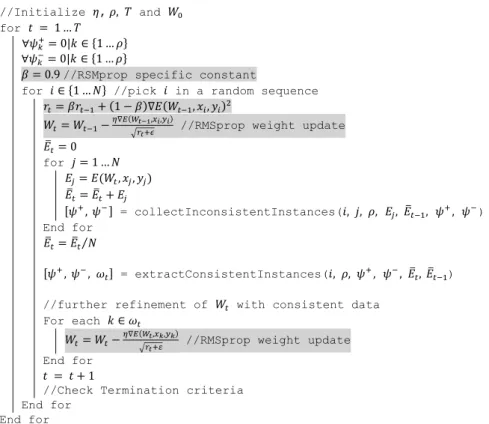
Since GSGD uses the same gradient computation formula, it has been easily incorporated into commonly used amendments for SGD; namely Adam, Adagdelta, Adagrad, RMSprop, Momentum and Nesterov. These amendments include some additional factors like momentum, regularization or variance reduction techniques [18]. To apply these variations to GSGD, only canonical weight update section in Fig. 4 needs to be replaced with the chosen variation of weight update. For example weight update for RMSprop is 𝑊𝑡= 𝑊𝑡−1− 𝜂

∇𝐸 ̅̅̅̅ √(𝑟𝑡+𝜀) , where 𝜀 = 1.0 × 10−8_,_and_𝑟 𝑡 = 𝛽𝑟𝑡−1+ (1 − 𝛽)∇𝐸̅̅̅̅𝑡 2

where 𝑟1= ∇𝐸̅̅̅̅1 and 𝛽 = 0.9. The guided

version of RMSprop is given in Fig. 7.

Gradient Computation (E)

Collect inconsistent data points for current iteration {ψ+_{, ψ}-_}

Weight Update ( W=-ηE)

Time for weight refinement? mod(i,ρ)==0 Extract promising consistent data points for current iteration {ψ+_{, ψ}-_}

No

All consistent data processed No Yes Yes Continue? No Yes

(13)

13

//Initialize 𝜂, 𝜌, 𝑇 and 𝑊0 for 𝑡 = 1 … 𝑇

∀𝜓𝑘+= 0|𝑘 ∈ {1 … 𝜌}

∀𝜓𝑘−= 0|𝑘 ∈ {1 … 𝜌}

𝛽 = 0.9 //RSMprop specific constant

for 𝑖 ∈ {1 … 𝑁} //pick 𝑖 in a random sequence

𝑟𝑡= 𝛽𝑟𝑡−1+ (1 − 𝛽)∇𝐸(𝑊𝑡−1, 𝑥𝑖, 𝑦𝑖)2

𝑊𝑡= 𝑊𝑡−1−

𝜂∇𝐸(𝑊𝑡−1,𝑥𝑖,𝑦𝑖)

√𝑟𝑡+𝜖 //RMSprop weight update

𝐸̅𝑡= 0 for 𝑗 = 1 … 𝑁 𝐸𝑗= 𝐸(𝑊𝑡, 𝑥𝑗, 𝑦𝑗) 𝐸̅𝑡= 𝐸̅𝑡+ 𝐸𝑗 [𝜓+_{, 𝜓}−_]_{= collectInconsistentInstances(}_{𝑖, 𝑗, 𝜌, 𝐸} 𝑗, 𝐸̅𝑡−1, 𝜓+, 𝜓−) End for 𝐸̅𝑡= 𝐸̅𝑡⁄𝑁 [𝜓+_{, 𝜓}−_{, 𝜔} 𝑡] = extractConsistentInstances(𝑖, 𝜌, 𝜓+, 𝜓−, 𝐸̅𝑡, 𝐸̅𝑡−1) //further refinement of 𝑊𝑡 with consistent data

For each 𝑘 ∈ 𝜔𝑡

𝑊𝑡= 𝑊𝑡−

𝜂∇𝐸(𝑊𝑡,𝑥𝑘,𝑦𝑘)

√𝑟𝑡+𝜀 //RMSprop weight update

End for

𝑡 = 𝑡 + 1

//Check Termination criteria End for

End for

Fig. 7.Pseudocode for Guided RMSprop

The highlighted lines show the only changes required to be done in GSDG to make it guided RMSprop. Rest of the code are same. Similarly, guided version for Adam, Adagdelta, Adagrad, Momentum and Nesterov have been created.

Finally, the convergence of GDAs has been discussed with constant learning rate and constraints associated with them. Using Taylor series for BGD the error function can be written as:

𝐸(𝑊_𝑡) ≤ 𝐸(𝑊_𝑡−1) + (𝑊_𝑡− 𝑊_𝑡−1)∇𝐸 = 𝐸(𝑊_𝑡−1) + (𝑊_𝑡−1− 𝜂∇𝐸 − 𝑊_𝑡−1)∇𝐸

∴ 𝐸(𝑊_𝑡) ≤ 𝐸(𝑊_𝑡−1) − 𝜂‖∇𝐸‖2 (8)

This shows that the error converges towards local optimum solution (global for convex function) gradually in every iteration. Large value of 𝜂 would result in divergence.

Similarly, error function for SGD can be written as: 𝐸(𝑊_𝑡) ≤ 𝐸(𝑊_𝑡−1) + (𝑊_𝑡− 𝑊_𝑡−1)∇𝐸

(14)

14

Here instead of the true gradient ∇𝐸, a randomly selected gradient for 𝑘𝑡ℎ_instance ∇𝐸(𝑊_𝑡−1, 𝑥𝑘 , 𝑦𝑘)has been used to update the weight 𝑊𝑡.

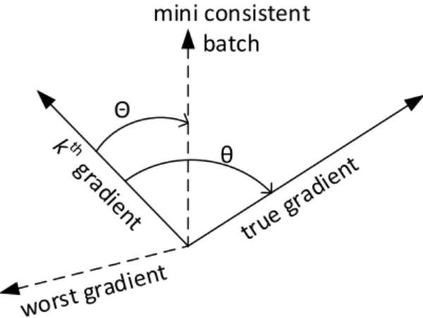
Fig. 8.Deviation of individual gradients from the true gradient

𝐸(𝑊_𝑡) ≤ 𝐸(𝑊_𝑡−1) − 𝜂∇𝐸(𝑊_𝑡−1, 𝑥𝑘 , 𝑦_𝑘) ∇𝐸 = 𝐸(𝑊𝑡−1) − 𝜂‖∇𝐸‖2𝑐𝑜𝑠𝜃

where 𝜃 is the angle between 𝑘𝑡ℎ gradient and the true gradient as shown in Fig. 8.

∴ 𝐸(𝑊_𝑡) ≤ {𝐸(𝑊𝑡−1), when consistent (𝜃 ≤ 𝜋 2) 𝐸(𝑊𝑡−1) + 𝜂‖𝛻𝐸‖2, when inconsistent (𝜃 > 𝜋 2) (9)

SGD would converge when the dataset is consistent, though convergence cannot be guaranteed due to high inconsistency present in the data set. This is the reason many fluctuations are seen during gradient descent. GSGD tries to reduce 𝜃 by selecting promising

instances that can bring𝑘𝑡ℎ gradient closer to the true gradient as shown by 𝛩 in Fig. 8. Since GSGD is an offshoot of SGD, its convergence is similar to SGD given in Eq. (9). The error value based on the algorithm defined in Fig. 4 and Fig. 5 can be given as:

𝐸(𝑊_𝑡) ≤ 𝐸(𝑊_𝑡−1) + (𝑊_𝑡−1− 𝜂 ∑ ∇𝐸(𝑊_𝑡−1(𝑖), 𝑥𝑖 , 𝑦_𝑖) |𝜔_𝑡|

𝑖=1 − 𝑊𝑡−1)∇𝐸

where 𝑊_𝑡−1(𝑖) refers to the intermediate weight value while processing the consistent set 𝜔_𝑡. ∴ 𝐸(𝑊_𝑡) ≤ 𝐸(𝑊_𝑡−1) − 𝜂‖∇𝐸‖2_{𝑐𝑜𝑠Θ}

and, 𝐸(𝑊_𝑡) ≤ {𝐸(𝑊𝑡−1), when consistent (Θ ≤

𝜋 2) 𝐸(𝑊𝑡−1) + 𝜂‖𝛻𝐸‖2, when inconsistent (Θ > 𝜋 2) (10)

By selecting promising instances the 𝑘𝑡ℎ gradient moves closer to the true gradient. GSGD will have better convergence with 𝛩 ≤ 𝜃.

mini consistent batch

θ Θ

(15)

15

5. Experiment

Since GSGD is simply a “guided” version of SGD, hence a comprehensive analysis was performed with guided version of canonical SGD, Adam, Adagrad, RMSprop, Adadelta, Momentum and Nesterov with their corresponding original versions. The coding was completely written in Matlab 2016. The experimental setup and execution have been discussed below:

5.1Test Data

The test data have been collected from various medical benchmark data sets available in UCI library [6]. The presence of inconsistency in datasets differs from each other; for instance, Breast Cancer Diagnostic has high consistency, Cancer and New Thyroid has medium level of consistency while rest of data sets are very chaotic.

To have a comparative analysis on the performance of algorithms, the quality metric is designed that consists of classification accuracy (CA) on a limited time budget, and number of function calls (NFC) for 30 successive runs on each data set. The algorithms are given sufficient and equal amount of time to converge where the algorithms are also monitored to not to overlearn.

The selected datasets belong to either two-class or multi-class classification problems. Since the GSGD differs from SGD mainly in prioritizing selection of consistent data for gradient computation, this may be argued as merely a kind of data preprocess with noise filtering. Hence, the algorithms have also been tested for both orientation of datasets i.e., without noise filtering and with noise filtering through outlier detection and removal. This demonstrates that even after noise filtering, GSGD performs better than SGD. Statistical inter-quartile range (IQR) outlier detection method available in [8] have been used to remove stochastic noise from datasets where CAs are low. This technique has been commonly used in medical domain with increased descriptive classification accuracy but with low predictive accuracy [14, 24]. The datasets are not intended to be free from the noise but to reflect the effect of some outlier removals in the tested algorithms.

(16)

16

5.2Parameter Settings

The experimental setup ensures that initial conditions like random order of training examples are same for both SGD and GSGD. Both algorithms are placed as subroutines inside the common loop of iterations. In this manner, same data instances are fed into the algorithms to make the comparison more reliable.

The parameter settings for SGD and GSGD are shown below in Table 1. Each algorithm was allowed to run for the maximum of 1000 iterations for 30 times. Due to small sized dataset 3-fold cross validation is done with 60:40 training-testing ratio. Neighborhood size (𝜌) should not be too large as it will make the algorithm less efficient. Additionally, it is important to choose the appropriate value of 𝜌 to avoid consistent instances becoming ‘stale’ and turning into inconsistent. GSGD’s convergence is similar to SGD’s where gradient descent happens more than once (for 𝜌 > 1) in every iteration.

Table 1.Parameter setting for GSGD and SGD

Parameter Value

Max iterations 1000

Attempts 30 consecutive runs Validation 3-fold cross validation Training:Testing ratio 60:40

Learning rate (𝜂) 0.2 Neighborhood size (𝜌) 10

5.3Parameter tuning

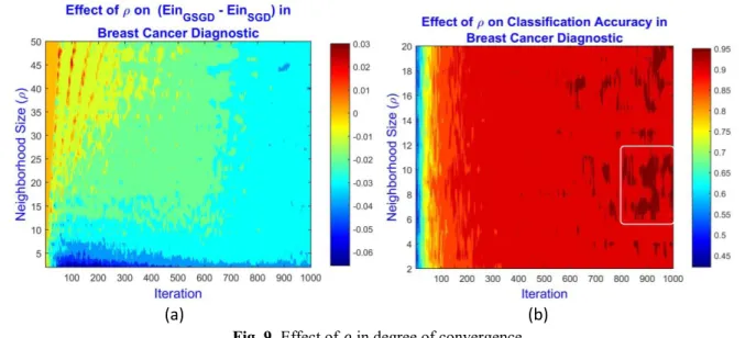
The degree of descent depends on learning rate, slope of the gradient, and also inconsistency present in a data set as shown in Eq. (7). Gradient descent with consistent instances happen after every 𝜌 iterations. To evaluate the influence of different values of 𝜌 in the degree of convergence, contour plot have been drawn for the difference of in-sample error between GSGD and SGD in Fig. 9 (a). The plot is based on the average of 30 runs with the same parameter settings defined in Table 1. The x-axis shows the number of iterations and y-axis shows the range of values for 𝜌 from 2 – 50. The lower the value of the contour plot, the better the performance of GSGD compared to SGD, and vice-versa. The selected data set was breast cancer diagnostic as it has produced smooth convergence for both SGD and GSGD, shown in Fig. 11. It is observed that 𝜌 ≤ 10 performs better compared to higher values of 𝜌.

(17)

17

Very low value of 𝜌 may seem to perform better with low in-sample error but its CA is also not very high. Fig. 9 (b) shows that 6 < 𝜌 < 11 have produced good CAs. Hence, parameter 𝜌 = 10 or little less is recommended to have a good convergence.

Non-parametric test was also performed with Wilcoxon test for ranking (two-tailed) to show null hypothesis with 𝑝 > 0.05 (there is no significance difference between tested algorithms)

is wrong. The test is conducted on 250th_{and 750}th_{iteration where insignificant difference are}

denoted by † and ‡ respectively in the result tables in the Appendix. Only in few instances it was shown that the guided and original algorithms have no significant difference. It may happen when the influence of inconsistent data is negligible or not many inconsistent data are present.

5.4Experiment Execution

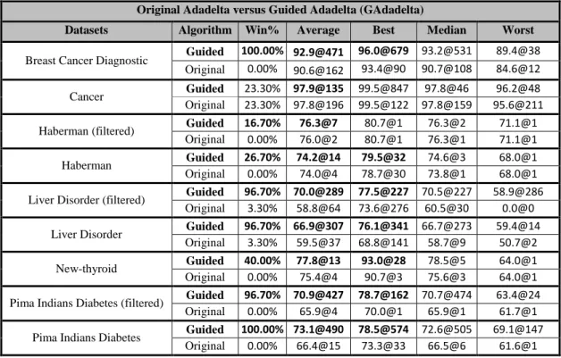
The comparative experimental results have been carried out between guided and original versions of the SGD algorithms. SGD has been tested against GSDG and similarly, Adadelta, Adagrad, Adam, Momentum, Nesterov, RMSprop have been tested against GAdadelta, GAdagrad, GAdam, GMomentum, GNesterov, and GRMSprop respectively. One to one comparison shows the influence of guided approach on a given original algorithm. The test results for the above mentioned algorithms are shown in the Appendix in Table A.1 – Table A.7 respectively. The datasets with removal of outliers are indicated as filtered datasets. The analysis is based on statistical testing of average, median, best and worst CAs together with Wilcoxon’s no significant difference indicator († and/or ‡). The first column shows the tested

(a) (b)

(18)

18

datasets, the second column indicates whether the algorithm is guided or original, and the third column indicates win%, which represents number of times guided (or original) algorithm got better result than the later (or former) out of 30 runs. Rest of the columns shows average, best, median and worst solutions with NFC after ‘@’ symbol. The better results between the two approaches are shown in bold letters. Guided approach has outperformed original approaches in almost all the algorithms. The empirical results definitely establishes that avoiding inconsistent training examples regularly produces better results. Furthermore, among the tested variations of SGD, Adam and RMSprop has mostly produced the best results.

6. Discussion

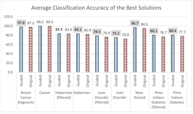
GSGD has not only outperformed SGD on its canonical version but also in all other popular variations of SGD. Due to the extent of experimental results, the outcomes have been summarized in Fig. 10 where each bar shows the average classification accuracy of the best solutions obtained by tested variations of SGD on a given problem. The highlighted values on the top of bars show notable improvement with the proposed guided approach such as Pima Indian Diabetes (filtered and non-filtered), where the improvement in classification accuracy

Fig. 10.Average classification accuracy of the best solutions for all the variations of SGD (and GSGD)

97.8 97.2 99.5 99.5 83.5 83.0 83.1 81.9 _78.5 76.0 75.1 _72.0 96.7 _94.5 80.1 _76.7 80.4 _77.7 0.0 20.0 40.0 60.0 80.0 100.0 120.0 G u id e d O ri gi n al G u id e d O ri gi n al G u id e d O ri gi n al G u id e d Ori gi n al G u id e d O ri gi n al G u id e d O ri gi n al G u id e d O ri gi n al G u id e d Ori gi n al G u id e d O ri gi n al Breast Cancer Diagnostic Cancer Haberman (filtered) Haberman Liver Disorder (filtered) Liver Disorder New-thyroid Pima Indians Diabetes (filtered) Pima Indians Diabetes

(19)

19

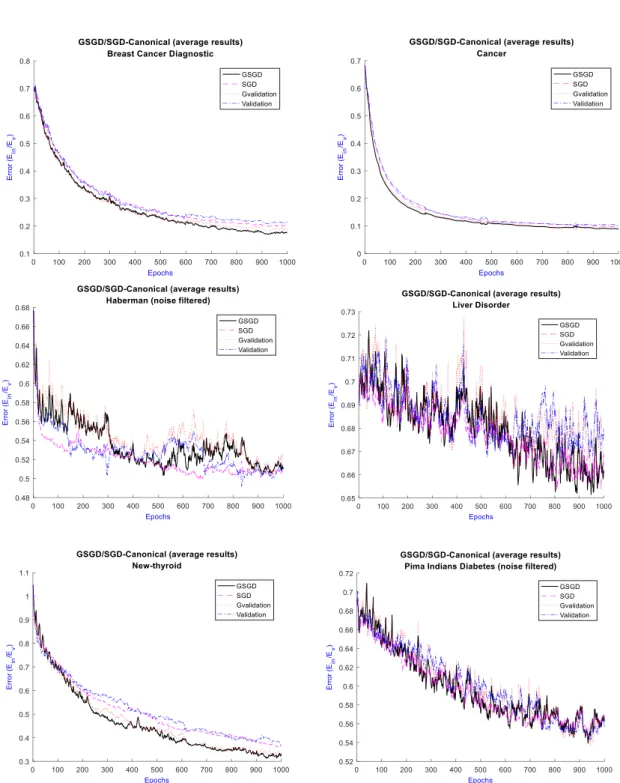
Fig. 11.Convergence graph of canonical SGD and GSGD for selected test problems

is by 3.4% and 2.7% respectively. Other notable improvement is shown in Liver Disorder (non-filtered and filtered) and New-thyroid, where classification accuracy is improved by 3.1%, 2.5% and 2.2% respectively. The selected graphs of convergence for canonical SGD and GSGD are shown in Fig. 11. The graphs show in-sample error (or training error) 𝐸𝑖𝑛 with

validation error 𝐸𝑣. Tracking of 𝐸𝑣 has been doneto avoid any over-fitting. Guided validation

(20)

20

Indians diabetes data sets are quite chaotic including filtered ones. Their best CAs are also quite low compared to the other problems, because of high bias (high training and testing error) and high variance with the chosen model. Additionally, they have high data inconsistency and insufficient data. It was also observed that even after removing the outliers and extreme values, GSGD has performed better than SGD. For rest of the problems, it is evident that the guided approach’s 𝐸𝑖𝑛 and 𝐸𝑣are lower than the original approach throughout

the training process. The purpose of GSGD is not to be used as an alternative or addition to the noise removal techniques, but to guide SGD when data inconsistency is high. Even if SGD would be used with a more complex model, most probably the testing error will not be improved unless sufficient and consistent data are provided.

7. Conclusion

This paper has introduced a guided search approach to improve canonical SGD, Adadelta, Adagrad, Adam, Momentum, Nesterov and RMSprop. The test results demonstrate that the guided approach has completely outperformed original approaches when used in logistic regression. In some cases, average classification accuracy has been improved by more than 3%. The proposed approach has realized that the inconsistent training examples leads to poorer classification accuracy. Additionally, its worst time complexity is also same as SGD’s

𝑂(𝑇(𝑑 + 𝑁)) and better than BGD’s 𝑂(𝑇𝑑𝑁). Hence, it can be very useful for training large

data sets efficiently. The future work would be to apply guided approach in deep learning and in asynchronous gradient descent where its efficiency should not be compromised. Guided approaches’ weakness could be the usage of additional memory and time to filter out inconsistent training examples. However, its effect is still needed to be seen on online learning/ensemble learning. Finally, a standard metrics and measurements are required to be accommodated for the presence of inconsistency in a training data set.

Acknowledgment

I would like to thank Dr. Vandana Sharma of Fiji National University, Fiji and Ms. Priynka Sharma of The University of the South Pacific, Fiji for proof reading this article and providing constructive feedback.

(21)

21

Bibliography

[1] Y. S. Abu-Mostafa, M. Magdon-Ismail, and H.-T. Lin, Learning From Data. S.l.: AMLBook, 2012.

[2] Y. Bengio, R. Ducharme, P. Vincent, and C. Jauvin, “A Neural Probabilistic Language Model,” Journal of Machine Learning Research, vol. 3, no. Feb, pp. 1137–1155, 2003. [3] C. M. Bishop, Neural Networks for Pattern Recognition. New York, NY, USA: Oxford

University Press, Inc., 1995.

[4] V. Chandola, A. Banerjee, and V. Kumar, “Anomaly Detection: A Survey,” ACM Comput. Surv., vol. 41, no. 3, pp. 15:1–15:58, Jul. 2009.

[5] J. Dean et al., “Large Scale Distributed Deep Networks,” in Advances in Neural Information Processing Systems 25, F. Pereira, C. J. C. Burges, L. Bottou, and K. Q. Weinberger, Eds. Curran Associates, Inc., 2012, pp. 1223–1231.

[6] D. Dheeru and E. Karra Taniskidou, UCI Machine Learning Repository. University of California, Irvine, School of Information and Computer Sciences, 2017.

[7] J. Duchi, E. Hazan, and Y. Singer, “Adaptive Subgradient Methods for Online Learning and Stochastic Optimization,” Journal of Machine Learning Research, vol. 12, no. Jul, pp. 2121–2159, 2011.

[8] Eibe Frank, Mark A. Hall, and Ian H. Witten, “The WEKA Workbench,” in Online Appendix for “Data Mining: Practical Machine Learning Tools and Techniques,” 4th ed., Morgan Kaufmann, 2016.

[9] M. T. Hoque, M. Chetty, and L. S. Dooley, “A new guided genetic algorithm for 2D hydrophobic-hydrophilic model to predict protein folding,” in 2005 IEEE Congress on Evolutionary Computation, 2005, vol. 1, pp. 259-266 Vol.1.

[10] Howard Anton, Irl Bivens, and Stephen Davis, “Partial Derivatives,” in Calculus, Early Transcendentals, 10th ed., USA: John Wiley & Sons, Inc., 2012, pp. 906–999.

[11] R. Johnson and T. Zhang, “Accelerating Stochastic Gradient Descent Using Predictive Variance Reduction,” in Proceedings of the 26th International Conference on Neural Information Processing Systems, USA, 2013, pp. 315–323.

[12] D. P. Kingma and J. Ba, “Adam: A Method for Stochastic Optimization,” arXiv:1412.6980 [cs], Dec. 2014.

[13] J. Konečný, J. Liu, P. Richtárik, and M. Takáč, “Mini-Batch Semi-Stochastic Gradient Descent in the Proximal Setting,” IEEE Journal of Selected Topics in Signal Processing, vol. 10, no. 2, pp. 242–255, Mar. 2016.

[14] J. Laurikkala, M. Juhola, and E. Kentala, “Informal Identification of Outliers in Medical Data,” in Fifth International Workshop on Intelligent Data Analysis in Medicine and Pharmacology, Berlin, Germany, 2000, pp. 20–24.

[15] Z. Michalewicz and D. B. Fogel, How to Solve It: Modern Heuristics, 2nd ed. Springer, 2004.

[16] M. Moreira and E. Fiesler, Neural Networks with Adaptive Learning Rate and

Momentum Terms. INSTITUT DALLE MOLLE D’INTELLIGENCE ARTIFICIELLE PERCEPTIVE, 1995.

[17] K. Murota, Discrete Convex Analysis: Monographs on Discrete Mathematics and Applications 10. Philadelphia, PA, USA: Society for Industrial and Applied Mathematics, 2003.

[18] N. Qian, “On the momentum term in gradient descent learning algorithms,” Neural Networks, vol. 12, no. 1, pp. 145–151, Jan. 1999.

[19] F. Rothlauf, Design of Modern Heuristics: Principles and Application, 1st ed. Springer Publishing Company, Incorporated, 2011.

(22)

22

[20] S. Ruder, “An overview of gradient descent optimization algorithms,” arXiv:1609.04747 [cs], Sep. 2016.

[21] S. J. Russell and P. Norvig, Artificial Intelligence - a modern approach, 2nd ed. New Jersey: Pearson Education Inc, 2003.

[22] A. Sharma, “Information Discovery from Constraints for Evolutionary Computational Model (Phd Dissertation),” University of Canberra, 2014.

[23] A. Sharma and D. Sharma, “ICHEA – A Constraint Guided Search for Improving Evolutionary Algorithms,” in In: Huang, T., Zeng, Z., Li, C., Leung, C.S. (eds.) ICONIP 2012, Part I. LNCS, Doha, Qatar, 2012, vol. 7663, pp. 269–279.

[24] H. E. Solberg and A. Lahti, “Detection of Outliers in Reference Distributions:

Performance of Horn’s Algorithm,” Clinical Chemistry, vol. 51, no. 12, pp. 2326–2332, Dec. 2005.

[25] C. Wang, X. Chen, A. J. Smola, and E. P. Xing, “Variance Reduction for Stochastic Gradient Optimization,” in Advances in Neural Information Processing Systems 26, C. J. C. Burges, L. Bottou, M. Welling, Z. Ghahramani, and K. Q. Weinberger, Eds. Curran Associates, Inc., 2013, pp. 181–189.

[26] D. R. Wilson and T. R. Martinez, “The general inefficiency of batch training for gradient descent learning,” Neural Networks, vol. 16, no. 10, pp. 1429–1451, Dec. 2003.

[27] Yaser S Abu-Mostafa, “Learning From Data - The Lectures,” Learning From Data, California Institute of Technology, 2016. [Online]. Available:

https://work.caltech.edu/lectures.html. [Accessed: 30-Aug-2016].

[28] C.-C. Yu and B.-D. Liu, “A backpropagation algorithm with adaptive learning rate and momentum coefficient,” in Proceedings of the 2002 International Joint Conference on Neural Networks, 2002. IJCNN ’02, 2002, vol. 2, pp. 1218–1223.

[29] Yurii Nesterov, “A method for unconstrained convex minimization problem with rate of convergence O(1/k2),” in Doklady AN SSSR (In Russian). (English translation. Soviet Math. Dokl, 1983.

[30] M. D. Zeiler, “ADADELTA: An Adaptive Learning Rate Method,” arXiv:1212.5701 [cs], Dec. 2012.

[31] S. Zheng et al., “Asynchronous Stochastic Gradient Descent with Delay Compensation,” in International Conference on Machine Learning, 2017, pp. 4120–4129.

[32] S. Zheng and J. T. Kwok, “Follow the Moving Leader in Deep Learning,” in International Conference on Machine Learning, 2017, pp. 4110–4119.

(23)

23

Appendix

Experimental results of guided and original SGD to compare classification accuracies

Table A.1.Classification accuracies of the canonical SGD against GSGD algorithm

Canonical SGD versus Guided SGD (GSGD)

Datasets Algorithm Win% Average Best Median Worst

Breast Cancer Diagnostic Guided 96.70% 96.8@684 98.7@542 96.5@663 95.2@809 Original 3.30% 95.9@471 98.2@610 95.6@515 93.8@575

Cancer Guided 13.30% 98.0@81 99.5@12 98.4@31 96.2@21

Original 10.00% 97.9@58 99.5@24 98.4@29 95.1@32

Haberman (filtered) ‡ Guided 70.00% 77.8@356 83.3@484 78.1@279 71.9@169 Original 0.00% 76.8@343 82.5@199 77.2@375 68.4@637

Haberman‡ Guided 70.00% 77.3@446 82.0@109 77.9@481 72.1@6

Original 0.00% 75.0@339 82.0@91 75.4@400 68.9@1

Liver Disorder (filtered) Guided 60.00% 71.4@557 76.7@679 71.3@616 65.9@805 Original 16.70% 70.2@368 76.7@416 70.2@385 63.6@544

Liver Disorder Guided 66.70% 66.5@445 73.9@196 65.9@435 62.3@406 Original 20.00% 65.4@365 71.0@516 65.6@380 60.9@665

New-thyroid Guided 86.70% 96.4@376 98.8@980 96.5@421 89.5@424

Original 3.30% 91.6@438 98.8@567 91.9@475 77.9@687

Pima Indians Diabetes (filtered) Guided 100.00% 77.2@695 82.2@907 77.4@733 74.2@576 Original 0.00% 75.1@511 79.4@614 75.1@546 72.5@606

Pima Indians Diabetes Guided 93.30% 77.8@629 81.1@255 78.0@631 74.6@210 Original 0.00% 76.1@458 80.1@628 76.4@496 72.3@20

Table A.2.Classification accuracies of the Adadelta against GAdadelta algorithm

Original Adadelta versus Guided Adadelta (GAdadelta)

Breast Cancer Diagnostic Guided 100.00% 92.9@471 96.0@679 93.2@531 89.4@38 Original 0.00% 90.6@162 93.4@90 90.7@108 84.6@12

Cancer Guided 23.30% 97.9@135 99.5@847 97.8@46 96.2@48

Original 23.30% 97.8@196 99.5@122 97.8@159 95.6@211

Haberman (filtered) Guided 16.70% 76.3@7 80.7@1 76.3@2 71.1@1

Original 0.00% 76.0@2 80.7@1 76.3@1 71.1@1

Haberman Guided 26.70% 74.2@14 79.5@32 74.6@3 68.0@1

Original 0.00% 74.0@4 78.7@30 73.8@1 68.0@1

Liver Disorder (filtered) Guided 96.70% 70.0@289 77.5@227 70.5@227 58.9@286 Original 3.30% 58.8@64 73.6@276 60.5@30 0.0@0

Liver Disorder Guided 96.70% 66.9@307 76.1@341 66.7@273 59.4@14

Original 3.30% 59.5@37 68.8@141 58.7@9 50.7@2

New-thyroid Guided 40.00% 77.8@13 93.0@28 78.5@5 64.0@1

Original 0.00% 75.4@4 90.7@3 75.6@3 64.0@1

Pima Indians Diabetes (filtered) Guided 96.70% 70.9@427 78.7@162 70.7@474 63.4@24

Original 0.00% 65.9@4 70.0@1 65.9@1 61.7@1

Pima Indians Diabetes Guided 100.00% 73.1@490 78.5@574 72.6@505 69.1@147

(24)

24

Table A.3.Classification accuracies of the Adagrad against GAdagrad algorithm

Original Adagrad versus Guided Adagrad (GAdagrad)

Cancer Guided 23.30% 97.7@90 99.5@322 97.8@32 96.2@18

Original 6.70% 97.6@70 99.5@245 97.8@31 96.2@24

Haberman (filtered) Guided 76.70% 78.4@252 84.2@202 78.9@172 71.9@1

Original 0.00% 76.5@33 84.2@483 75.4@1 70.2@1

Haberman Guided 86.70% 76.3@240 83.6@125 76.2@178 66.4@257

Original 0.00% 74.0@119 80.3@82 73.8@8 65.6@1

Liver Disorder (filtered) † Guided 83.30% 71.9@545 78.3@223 71.7@596 62.8@928 Original 6.70% 69.4@338 74.4@302 70.2@296 58.1@197

Original 6.70% 65.5@228 72.5@66 65.2@171 57.2@23

New-thyroid Guided 100.00% 90.1@519 97.7@86 90.1@603 83.7@897

Original 0.00% 82.6@493 87.2@619 82.6@503 76.7@488

Pima Indians Diabetes (filtered) Guided 96.70% 72.4@531 78.0@459 72.5@579 68.6@584 Original 3.30% 69.7@296 74.6@99 69.3@282 64.8@365

Pima Indians Diabetes† Guided 100.00% 72.7@669 76.9@138 72.5@746 69.4@807 Original 0.00% 68.9@299 73.6@378 68.4@319 63.2@469

Table A.4.Classification accuracies of the Adam against GAdam algorithm

Original Adam versus Guided GAdam (GAdam)

Breast Cancer Diagnostic Guided 56.70% 97.9@657 99.1@871 98.2@684 95.2@867 Original 13.30% 97.5@507 99.1@397 97.8@534 95.2@620

Cancer†‡ Guided 23.30% 98.0@279 100.0@9 98.1@197 96.7@220

Original 0.00% 97.9@258 100.0@9 97.8@216 96.2@11

Haberman (filtered) †‡ Guided 46.70% 80.1@353 84.2@388 80.3@262 74.6@585 Original 10.00% 79.5@280 83.3@343 79.8@329 72.8@351

Haberman† Guided 33.30% 79.5@451 86.9@518 79.5@344 73.0@761

Original 10.00% 79.2@303 86.9@395 79.5@311 71.3@47

Liver Disorder (filtered) † Guided 40.00% 74.3@555 79.8@201 74.4@588 69.8@653 Original 30.00% 73.9@372 79.8@556 74.0@337 70.5@517

Liver Disorder Guided 60.00% 71.8@598 76.1@821 71.7@664 63.8@321

Original 13.30% 70.8@372 76.1@269 71.0@363 63.0@130

New-thyroid Guided 23.30% 98.6@378 100.0@699 98.8@232 95.3@877

Original 13.30% 98.4@353 100.0@436 98.8@375 94.2@398

Pima Indians Diabetes (filtered) † Guided 80.00% 77.3@662 80.8@802 77.2@648 74.2@433 Original 16.70% 76.4@494 79.8@491 76.7@490 73.2@652

Pima Indians Diabetes Guided 70.00% 77.8@692 81.4@734 77.7@725 74.6@832 Original 16.70% 76.8@545 81.1@678 76.7@564 73.6@619

(25)

25

Table A.5.Classification accuracies of the Momentum against GMomentum algorithm

Original Momentum versus Guided Momentum (GMomentum)

Cancer Guided 6.70% 97.9@80 99.5@18 97.8@29 96.7@45

Original 6.70% 97.9@76 99.5@16 97.8@29 96.7@31

Haberman (filtered) ‡ Guided 76.70% 79.3@364 86.0@190 79.8@333 71.1@8 Original 0.00% 78.2@405 84.2@463 78.1@462 71.1@8

Haberman‡ Guided 83.30% 77.8@454 85.2@159 77.9@327 70.5@1

Original 3.30% 75.1@282 83.6@215 74.6@360 68.9@5

Liver Disorder (filtered) Guided 63.30% 68.9@631 80.6@506 69.0@630 62.8@204 Original 20.00% 68.2@407 78.3@455 69.8@441 62.0@637

Original 20.00% 65.2@382 71.0@345 65.6@371 57.2@164

New-thyroid Guided 90.00% 96.8@566 100.0@387 97.7@538 93.0@179

Original 0.00% 91.5@402 98.8@258 91.9@407 82.6@30

Pima Indians Diabetes Guided 80.00% 75.7@567 80.5@755 75.6@580 72.3@551 Original 6.70% 74.7@418 79.2@163 74.4@424 71.3@429

Table A.6.Classification accuracies of the Nesterov against GNesterov algorithm

Original Nesterov versus Guided Nesterov (GNesterov)

Cancer Guided 13.30% 97.7@60 98.9@18 97.8@28 96.7@122

Original 6.70% 97.7@46 98.9@33 97.5@26 96.7@20

Haberman (filtered) Guided 6.70% 74.9@3 79.8@1 75.4@1 70.2@1

Original 3.30% 74.9@2 79.8@1 75.4@1 70.2@1

Haberman Guided 30.00% 74.5@28 82.8@297 73.8@2 68.9@3

Original 3.30% 74.0@3 79.5@23 73.8@1 68.9@3

Liver Disorder (filtered) Guided 100.00% 70.7@612 77.5@712 71.3@716 64.3@723

Original 0.00% 60.0@90 69.8@31 59.3@48 50.4@4

Original 0.00% 59.9@47 68.8@118 59.4@22 54.3@1

New-thyroid Guided 43.30% 78.9@132 87.2@27 79.7@9 68.6@31

Original 3.30% 76.8@5 86.0@9 76.2@2 65.1@1

Pima Indians Diabetes (filtered) Guided 96.70% 74.1@485 77.7@692 74.4@546 70.0@163

Original 0.00% 67.6@32 74.2@22 67.9@5 61.0@1

Pima Indians Diabetes Guided 100.00% 75.2@493 81.8@824 74.8@478 71.0@891

(26)

26

Table A.7.Classification accuracies of the RMSprop against GRMSprop algorithm

Original RMSprop versus Guided RMSprop (GRMSprop)

Breast Cancer Diagnostic Guided 70.00% 96.3@706 98.2@371 96.5@767 94.3@714 Original 13.30% 95.8@560 98.7@668 95.8@622 93.8@665

Cancer Guided 13.30% 97.9@212 99.5@317 97.8@72 96.2@26

Original 3.30% 97.8@169 99.5@636 97.8@59 96.2@79

Haberman (filtered) †‡ Guided 60.00% 81.2@408 86.0@145 81.6@315 74.6@5 Original 3.30% 80.6@253 86.0@479 80.7@278 74.6@5

Haberman †‡ Guided 50.00% 78.1@451 82.0@299 78.7@378 73.0@926

Original 3.30% 77.5@249 82.0@242 78.3@239 72.1@57

Liver Disorder (filtered) Guided 73.30% 74.3@515 79.1@790 75.6@524 67.4@211 Original 13.30% 73.3@411 79.1@162 73.6@464 65.9@530

Original 10.00% 71.7@452 76.1@306 72.1@502 63.0@164

New-thyroid Guided 46.70% 98.4@488 100.0@841 98.8@468 95.3@191

Original 3.30% 97.9@277 100.0@284 97.7@224 95.3@207

Pima Indians Diabetes Guided 93.30% 77.1@694 82.7@744 77.0@741 73.6@424 Original 3.30% 75.5@574 81.8@646 75.6@646 71.7@351