Variable indicators for optimum wavelength selection in diffuse
re
fl
ectance spectroscopy of soils
M.C. Sarathjith
a,⁎
, Bhabani Sankar Das
b, Suhas P. Wani
c, Kanwar L. Sahrawat
c aInternational Crops Research Institute for the Semi-Arid Tropics, Bamako BP-320, Mali
bAgricultural and Food Engineering Department, Indian Institute of Technology Kharagpur, West Bengal 721302, India c
International Crops Research Institute for the Semi-Arid Tropics, Patancheru, Hyderabad, Telangana 502324, India
a b s t r a c t
a r t i c l e i n f o
Article history: Received 27 June 2015
Received in revised form 23 December 2015 Accepted 29 December 2015
Available online xxxx
Diffuse reflectance spectroscopy (DRS) operating in 350–2500 nm wavelength range is fast emerging as a rapid and non-invasive technique for analyzing multiple soil attributes. Because the spectral reflectance values in this range of wavelengths are highly co-linear, it is important to select relevant spectral information from the reflectance spectra to build a robust spectral algorithm. The objective of this study is to examine the utility of different variable indica-tors such as partial least squares regression (PLSR) coefficients (β), variable influence on projection, squared residual (SqRes), correlation coefficient (r), biweightmidcorrelation (bicor), mutual information based adjacency value (AMI), signal-to-noise ratio (StN), covariance procedures (CovProc) and their combinations in conjunction with an ordered predictor selection (OPS) approach for selecting optimum number of spectral variables (NSV) which could improve DRS model performance. The approach was tested with the PLSR models of pH, organic carbon, extractable iron (Fe), sand and clay contents and geometric mean diameter in Vertisols and Alfisols. The prediction accuracy of best models selected via OPS approach was found to be superior to full-spectrum (NSV = 2048) model for all the soil attributes. The percent decrease in RMSE value was found to be highest for Fe (14%, NSV = 79) in Alfisols followed by pH (9%, NSV = 660) in Vertisols while it varied between 3 and 8% for other soil attributes. Although the results were not conclusive in favor of one specific variable indicator, theCovProcandbicorwere found to be more appro-priate for accurate and moderate DRS models in this study, respectively. The overall results of this study advocate the use of OPS approach with variable indicators and their combinations as a promising strategy to develop simple and effective DRS models for soils.
© 2015 Elsevier B.V. All rights reserved. Keywords:
Diffuse reflectance spectroscopy Variable indicator
Ordered predictor selection Partial least squares regression Spectral variables
1. Introduction
Over the last few decades, diffuse reflectance spectroscopy (DRS) has been recognized as a rapid and non-invasive technique for the measurement of multiple soil attributes. The DRS approach is also widely adapted as a digital soil mapping tool across the globe (Ben-Dor and Banin, 1995; Soriano-Disla et al., 2014). Typically, an efficient multivari-ate regression model is developed between targeted soil attributes and spectral reflectance values in visible to near- and shortwave-infrared (VisNIR) range of wavelengths (350–2500 nm) in the DRS approach. Both linear and non-linear chemometric and data mining algorithms such as principal components regression, partial least squares regression (PLSR), support vector regression (Thissen et al., 2004), regression trees (Brown et al., 2006), multivariate adaptive regression splines (Shepherd and Walsh, 2002), committee trees (Vasques et al., 2009b), artificial neural networks (Daniel et al., 2003; Goldshleger et al., 2012) have been examined in soil DRS studies. Among these, the PLSR approach seems most frequently used because of its ability to address multicollinearity
of spectral variables, interpretability and computational performance (Viscarra Rossel et al., 2006; Stenberg et al., 2010). Performance of these models relies on their capability to extract important spectral characteris-tics or features (e.g., electronic transitions, overtones and combinations of fundamental vibrations in the mid-infrared frequencies) relevant to the soil attribute of interest (Viscarra Rossel et al., 2006; Viscarra Rossel and Lark, 2009).
A general practice in the DRS approach is the use of either entire (full-spectrum) or selected reflectance values as spectral variables for building a DRS model. The VisNIR response is generally weak and consists of complex absorption features (Stenberg et al., 2010). Hence, the selection of either a full or a part of the spectrum without a proper guideline often leads to have redundant or irrelevant information in the DRS model affecting its performance. The selection of appropriate and optimum number of spectral variables is expected to reduce model complexity and improve robustness (Xiaobo et al., 2010) and prediction accuracy of calibration models (Jouan-Rimbaud et al., 1995; Nadler and Coifman, 2005).Fernández Pierna et al. (2009)suggested that a robust variable selection method should yield a small set of variables capable of providing better, or at least, equivalent model performance to those obtained by the original set of variables. Hence, variable selection
⁎ Corresponding author.
E-mail addresses:[email protected],[email protected](M.C. Sarathjith).
http://dx.doi.org/10.1016/j.geoderma.2015.12.031
0016-7061/© 2015 Elsevier B.V. All rights reserved.
Contents lists available atScienceDirect
Geoderma
should be included as a critical step in DRS data analysis routine to accomplish the aforesaid advantages. A few sophisticated variable selection approaches (Xiaobo et al., 2010) have already been examined in the spectroscopic studies including successive projections algorithm (Araújo et al., 2001), uninformative variable elimination (Centner et al., 1996), simulated annealing (Kirkpatrick et al., 1983), genetic algorithms (Leardi et al., 1992), moving window partial least square (Chen et al., 2011), interval partial least squares (Norgaard et al., 2000), backward variable selection for PLSR (Fernández Pierna et al., 2009), wavelet transformation (Ge and Thomasson, 2006) among others. Recently,Li et al. (2009)developed a competitive adaptive reweighted sampling (CARS) as a strategy for spectral variable selection using regression coefficient (β) of PLSR model.Vohland et al. (2014) success-fully implemented the CARS approach in the soil dataset, and concluded that the approach is simple, accurate, and involves reasonable and parsimonious variable selection. However, no unique solution exists for this approach, mainly because of the Monte Carlo strategy and random numbers used in CARS. The issue may be resolved with the use of‘variable indicators’or‘informative vectors’in conjunction with an ordered predictor selection (OPS) approach, as suggested byTeófilo et al. (2009). In addition, the OPS approach has the following advantages: simple,flexible, effective in parsimonious selection and interpretability of spectral variables. The OPS approach has not been tested with soil datasets for a multitude of variable indicators.
In general, the variable indicators are descriptors of the relationships between predictor (spectral variables) and response (soil attribute) vari-ables. The information on the predictors–response relationship conveyed by each variable indicator differs by the underlying mathematical princi-ple or operation that guides their calculation. Thus, variable indicators may be considered appropriate for optimum spectral variable selection. In spectroscopy, several variable indicators exist (Teófilo et al., 2009), which may be broadly classified into PLSR-dependent and PLSR-independent categories. Theβ, variable influence on projection (VIP), squared residual vector (SqRes) and net analyte signal (NAS) are PLSR-dependent variable indicators, while correlation vector (r), signal-to-noise vector (StN) and covariance procedures vector (CovProc) are independent of PLSR model in their calculation. The co-efficient vectorβis a linear measure that represents the expected change in the response per unit change in the predictor variable (Mosteller and Tukey, 1977), whereasVIP(Wold et al., 1993) represents the importance of a predictor variable on the model based on the weighted PLSR coefficients. Variable indicatorSqRes(Teófilo et al., 2009) represents the difference between the original and reconstructed spectra, which has relevant information on the important spectral variables. Variable indicatorNASis defined as the part of the spectrum unique to the attribute of interest (Ferré and Faber, 2003), and is similar toβfor inverse calibration algorithms (Teófilo et al., 2009). The indica-torrrepresents the Pearson correlation coefficients. TheStN(Brown, 1992) denotes signal-to-noise statistics for each variable generated by least squaresfit between predictor variables to the response variable. The indicatorCovProc(Reinikainen and Hoskuldsson, 2003) represents the diagonal values of covariance matrix as a measure of strength between predictors and response variable. New vectors could be gener-ated by combining different variable indicators following normalization (Teófilo et al., 2009).
To the best of our knowledge, the utility of variable indicators in spectral variables selection has been limited toβ (Vohland et al., 2014), whileVIPandrhave been mainly used for feature visualization in soil DRS studies.Vohland et al. (2014)have cross-validated the use ofβand emphasized the need for an independent validation for its use in optimum variable selection. In addition, the elemental values of
βare highly dependent on the number of latent variables used in the model (Teófilo et al., 2009), and hence assumed to be less stable compared to the PLSR-independent counter parts. The utility of other PLSR-dependent, independent and their combinations in spectral variables selection is rarely examined, and thus warrants further
investigation. Thus, the objectives of this study are a) to evaluate the performance of OPS approach in the optimum spectral variables selection using different variable indicators, and b) to identify the best variable indicator for optimum spectral variable selection for each soil attribute.
2. Materials and methods 2.1. Soil samples and their analyses
Soil samples examined in this study were those used bySarathjith et al. (2014a, 2014b). Briefly, the surface (0–10 cm) soil samples were collected from 25 contiguous villages from the northern Karnataka (sampled area: 9839 km2) and 25 villages from southern Karnataka
(sampled area: 2602 km2). In general, soils in northern Karnataka are
classified as Vertisols and those in the southern Karnataka as Alfisols. Vertisols in Karnataka generally occur as Vertisols with intergrades and a mixture of Vertic Inceptisols. These soil groups are distinctly different with regard to pH, iron oxides, clay mineral, cation exchange capacity, silica-sesquioxide ratio and parent material (Lotse et al., 1972). The chemical, physical and spectral attributes of soils were estimated using that fraction which sifted through 2 mm sieve after air drying and manual grinding. Soil samples were subjected to the chemical analyses routine for the determination of pH by potentiometric means using a 1:2.5 soil/water ratio; organic carbon (OC) by the dichro-mate oxidation method (Walkley and Black, 1934); and extractable iron (Fe) content using inductively coupled plasma optical emission spectrometry (ICP-OES, HD Prodigy, Leeman Labs, New Hampshire, USA). The physical attributes examined in this study include soil particle size (clay and sand content) measured by pipette method (Gee and Bauder, 1986) and geometric mean diameter (GMD) by dry sieving of soil samples in a stack of eight sieves (Sarathjith et al., 2014a). These soil attributes cover a range of chemical and physical chromophores frequently estimated in the DRS approach.
A portable spectroradiometer (Field Spec 3 FR, Analytical Spectral Devices Inc.) equipped with a contact probe of 10 mm spot size was used to record the proximal spectral reflectance (350–2500 nm) from a leveled surface (Mouazen et al., 2010) of about 50 g soil sample placed in an aluminum moisture box (10 cm diameter). Soil reflectance was measured from each quadrant of the moisture box. White reference spectrum from a Spectralon (Labsphere) panel (9.2-cm diameter) was acquired before scanning each soil sample (Sarathjith et al., 2014b).
Table 1
Descriptive statistics of soil attributes.
Soil attribute Calibration Validation
n Mean Range n Mean Range Vertisols pH 175 8.57 (5)a 6.63–9.60 58 8.56 (5) 6.65–9.23 OC, % 175 0.39 (37) 0.14–0.93 58 0.39 (36) 0.15–0.76 Fe, mgL−1 175 7.22 (78) 1.70–29.60 59 7.03 (76) 1.70–28.30 Sand, % 178 66.39 (13) 44.51–84.82 60 66.18 (13) 44.71–84.21 Clay, % 176 14.45 (30) 4.47–35.27 59 14.52 (32) 6.43–33.30 GMD 176 0.31 (23) 0.17–0.49 59 0.31 (24) 0.17–0.49 Alfisols pH 175 6.68 (21) 4.30–9.50 58 6.65 (20) 4.40–8.80 OC, % 174 0.37 (33) 0.11–0.75 58 0.37 (33) 0.12–0.70 Fe, mgL−1 175 14.87 (86) 2.00–104.80 58 14.19 (75) 2.60–40.00 Sand, % 174 78.85 (9) 53.30–91.60 58 78.73 (9) 55.00–90.40 Clay, % 178 12.72 (51) 3.70–34.30 59 12.49 (49) 3.90–28.50 GMD 175 0.21 (25) 0.13–0.45 58 0.21 (24) 0.13–0.37 n: Number of soil samples.
a
2.2. Data processing and development of full-spectrum PLSR models All necessary data analyses were performed using MATLAB (R2012a, The Mathworks) software. Initially, Kolmogorov–Smirnov (KS) test statistic at the 5% significance level was performed to evaluate the normality in the frequency distribution of soil attributes. Soil attributes failing theKStest were subjected to natural logarithm or Box–Cox transformation in sequence, and further evaluated for normality. Soil attributes with skewed distribution even after transformations were left untransformed.
Four reflectance spectra from a soil sample were smoothed using a third-order Savitsky–Golayfiltering algorithm with 9 nm span length (Vasques et al., 2009a) and averaged to have a representative spectrum of the soil. The tail ends of the spectrum were discarded due to poor signal/noise ratio and the reflectance values between 400 and 2447 nm (full-spectrum) were used for further data modeling. Later, the refl ec-tance values were subjected tofirst derivative (FD) transformation as it was found to be more appropriate for these soil datasets (Sarathjith et al., 2014b). Principal component regression relationships were developed between soil attributes andFDspectra and the residuals were examined (at 5% level of significance) for the detection and removal of outlier samples. The remaining soils were divided into calibration and validation data sets in 3:1 ratio using‘sorting’algorithm (Viscarra Rossel and Lark, 2009). Every forth sample starting from second of soil attribute values arranged in ascending order was treated as validation samples, while the remaining samples were used for calibration. The similarity (at 5% level of significance) of mean and variance between data subsets was evaluated using two-parameter Student'st-test and Levene'sF-test, respectively. The PLSR model representing the relationship between soil attribute andFDreflectance, was built with the calibration dataset and tested using validation samples. Leave-one-out cross-validation approach was implemented tofind the optimum number of latent variables for the PLSR model (Viscarra Rossel, 2007). The model evaluation was based on the coefficient of determination (R2), root mean squared error (RMSE),
and the residual prediction deviation (RPD). Based on RPD value of validation, all DRS models were classified as accurate (RPDN2), moderate (1.4NRPDb2) and poor (RPDb1.4), as suggested by Chang et al. (2001).
2.3. Spectral variable indicators used in this study
The spectral variable indicators examined in this study includeβ, VIP,SqRes(PLSR-dependent),r, biweightmidcorrelation vector (bicor),
mutual information based adjacency vector (AMI),StNandCovProc (PLSR-independent). Generally, significant spectral variables (wave-lengths) have high absolute magnitude for all variable indicator values withSqResas an exception. The elements ofSqReswith low absolute values are significant (Teófilo et al., 2009) and hence, the reciprocal of SqReswas used for all the subsequent analyses. To the best of our knowledge, the spectral variable indicators namely,SqRes,StN, and CovProchave yet not been applied in thefield of soil spectroscopy. Further, no spectroscopic studies have implemented bothbicorand AMI(Sarathjith et al., 2014b; Song et al., 2012; Wilcox, 2005) as spectral variable indicators. Calculation and details on the spectral variable indicators used have been described inTeófilo et al. (2009)and Sarathjith et al. (2014b).
In addition, a combination of aforementioned indicators was also used as spectral variable indicators, as suggested byTeófilo et al. (2009). Accordingly, new sets of spectral variable indicators were generated by pair-wise combination of a) PLSR-dependent indicators only (3 combinations), and b) PLSR-dependent and independent indica-tors (15 combinations). Each spectral variable indicator in a pair was subjected to standard normal variate transformation. The combined indicator was the result of element wise product of absolute values of the normalized spectral variable indicators. Thus, a total of 26 spectral variable indicators (8 individual + 18 combinations) were examined in this study.
2.4. OPS approach
Selection of optimum number of spectral variables (NSV) using variable indicators was performed by means of an OPS approach similar to that reported byTeófilo et al. (2009). The OPS approach in this study employed an exponential decrease function (EDF) to select number of spectral variables (Li et al., 2009) against the uniform interval based wavelength selection inTeófilo et al. (2009). Initially, the normalized variable indicator was sorted in the decreasing order of their absolute magnitude. It was followed by a forced removal of wavelengths with relatively low absolute magnitude using the EDF of the formricomputed
as given below:
ri¼aexpð−kðiþ1ÞÞ ð1Þ
k¼ ln 0ð :5pÞ
m−1 ð2Þ
a¼ð0:5pÞ1=ðm−1Þ ð3Þ
wherei= 1,2,3,…,mrepresents the iteration number withmset to 50 andpis the total number of spectral variables. The use of EDF enables a Table 2
Regression statistics for the prediction of soil attributes using full-spectrum range (LV: number of latent variables, R2
: coefficient of determination, RMSE: root mean squared error, RPD: residual prediction deviation).
Soil attribute LV Calibration Validation
R2 RMSE RPD R2 RMSE RPD Vertisols pHc 9 0.89 0.14 3.06 0.78 0.21 2.14 OCa 8 0.81 0.16 2.30 0.57 0.24 1.54 Feb 10 0.92 0.09 3.58 0.78 0.15 2.17 Sand 5 0.62 5.21 1.62 0.55 5.61 1.51 Claya 5 0.64 0.18 1.68 0.47 0.22 1.39 GMD 8 0.87 0.03 2.76 0.80 0.03 2.24 Alfisols pHc 10 0.93 0.37 3.74 0.87 0.48 2.81 OC 10 0.79 0.06 2.19 0.56 0.08 1.53 Fea 4 0.68 0.44 1.78 0.68 0.43 1.79 Sandc 4 0.78 3.38 2.14 0.74 3.71 1.99 Claya 8 0.84 0.21 2.47 0.80 0.22 2.27 GMDa 11 0.90 0.07 3.16 0.77 0.11 2.09 a
Soil properties subjected to natural logarithm transformation. b
Soil properties subjected to Box–Cox transformation. c
Soil properties where transformations failed and data remained untransformed.
‘fast selection’of variables in the beginning followed by a‘refined selection’in the subsequent iterations (Li et al., 2009). Then,mnumber of DRS models (hereinafter, referred to as‘subset models’) with differ-ent NSV were generated. The NSV to be retained for generating subset models was defined by the product ofriandp. All the subset models
were trained and tested using the same samples used for the calibration and validation of full-spectrum model, respectively. The maximum number of latent variables to be used in subset models was limited to its optimum number obtained for full-spectrum model (Vohland et al., 2014). The performance of subset models was evaluated based on minimum-RMSE criterion in validation dataset. The subset model that
yields low RMSE was treated as the optimum model and the respective NSV as the optimum NSV for the chosen soil attribute using a variable indicator. All the aforementioned steps were performed using all vari-able indicators for each soil attribute in both the soil groups.
3. Results and discussion
3.1. Descriptive statistics of soil attributes
The descriptive statistics of the soil attributes in calibration and validation dataset for both Alfisols and Vertisols are given inTable 1.
Fig. 2.Comparison of full-spectrum and optimum models for each variable indicator namely,β: regression coefficient,VIP: variable influence on projection,SqRes: squared residual vector, r: Pearson correlation coefficients,bicor: biweightmidcorrelation vector,AMI: mutual information based adjacency vector,StN: signal to noise ratio,CovProc: covariance procedure and their pairwise combinations.
Both soil groups used are distinctly different for all soil attributes, except for OC. The pH value indicates the slight acidic and alkaline nature of Alfisols and Vertisols, respectively. Based on the USDA soil textural classification system, sandy loam soils (78%) were prominent in Vertisols while loamy sand (41%) and sandy loam (36%) soils together accounted for the major share in Alfisols. The Vertisols were found to have low Fe content compared to that of Alfisols. Low clay contents in Vertisols may have resulted from associated intergrades and Vertic Inceptisols. The similar values in the OC distribution for both the soil groups represent the low carbon status of semiarid tropical regions. The data partitioning approach implemented in the study ensured sim-ilarity in the distribution of samples between calibration and validation dataset for all soil attributes with regard to their mean and variance, as evaluated using Student'st-test and Levene'sF-test, respectively. The approach was also successful in confining the extremas of validation within the range of calibration datasets for most of the soil attributes. A validation sample in Fe (104.70 mgL−1) and sand content (87.82%)
of Vertisols with value outside the range of calibration was excluded from the subsequent analyses.
3.2. Prediction of soil attributes using full-spectrum PLSR models
Table 2summarizes the model calibration and prediction results of soil attributes in Alfisols and Vertisols. The regression statistics for the calibration and validation of full-spectrum based PLSR models were comparable to those reported in the literature for pH (Kinoshita et al., 2012; Tekin et al., 2012), OC (Bayer et al., 2012; Morgan et al., 2009; Stevens et al., 2006), Fe (Abdi et al., 2012; Bayer et al., 2012), sand content (Kinoshita et al., 2012; Viscarra Rossel and Webster, 2012), clay content (Ben-Dor and Banin, 1995; Brown et al., 2006) and GMD (Sarathjith et al., 2014a) in both the soil groups. Accurate predictions were noted for pH, sand and clay contents, GMD in Alfisols, and pH, GMD in Vertisols. The prediction of clay contents in Vertisols was found to be poor, while all the remaining attributes in both soil groups were estimated with moderate accuracy.
3.3. Selection of optimum number of spectral variables
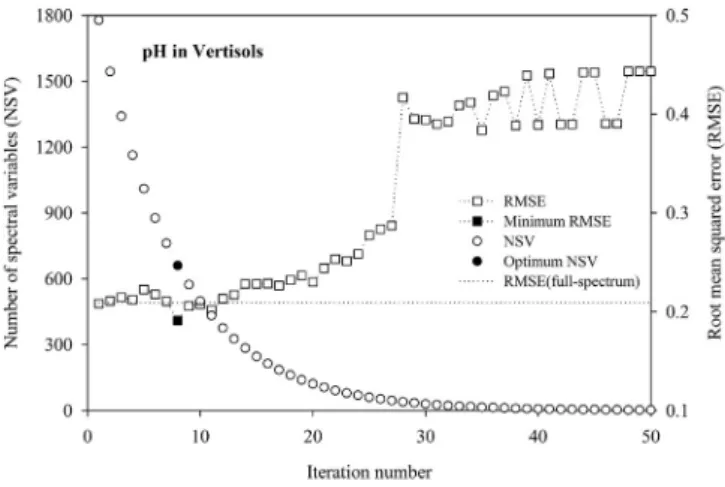
The OPS plot for the selection of model with optimum NSV is shown inFig. 1for pH in Vertisols usingCovProcas variable indicator as an illustrative example. Typical variations in RMSE value of validation dataset for subset models with different NSV are shown in the OPS
plot. Subset models in thefirst few iterations (1 to 13) yielded similar or even lower RMSE values compared to full-spectrum models. This revealed that the spectral variables eliminated in those iterations were noisy or least significant for model performance. Thereafter, an increase in the RMSE values was noted for the subsequent models (iteration number from 14 to 27), which may be attributed to the removal of infor-mative spectral variables. The performance of subset models with most significant spectral variables alone (after iteration number 28) was found to be always poor. Based on minimum-RMSE criterion, the subset model at iteration number 8 was found to be optimum (RMSE = 0.19; NSV = 660) for pH in Vertisols usingCovProcas variable indicator. Similarly, the regression statistics of subset models with optimum NSV (hereinafter, referred to as the optimum model) for different variable indicators were compiled for selecting best variable indicator for each soil attribute.
3.4. Selection of best variable indicator
Fig. 2shows the percent difference in RMSE values between full-spectrum model and optimum models using different variable indica-tors for all soil attributes of Vertisols and Alfisols. The baseline value of zero corresponds to the RMSE of full-spectrum model. The negative and positive bars represent the improvement and deterioration (possibly, information loss) in the prediction accuracy accomplished with the OPS approach, respectively. The selection of best variable indicator was based on both the model accuracy (in terms of RMSE) and complexity (in terms of NSV). Initially, all the optimum models with RMSE value within 5% proximity (in magnitude) to the lowest RMSE were selected. Among these, the model with low NSV was treated as the best model and respective variable indicator as the‘best’for the soil attribute. For example, the combination of variable indicatorsβandVIP(β–VIP) yielded high accuracy (RMSE = 0.45; NSV = 573) compared to all other variable indicators in the case of pH in Alfisols (Fig. 2). ButVIP–CovProc combina-tion should instead be treated as the best variable indicator because it gives almost similar prediction (RMSE = 0.46) to that given byβ–VIP combination (within 5% difference) at low NSV (NSV = 245). If no values are found within the proximity of lowest RMSE, then the best variable indicator should be the one that yields low RMSE as is the case of pH, OC in Vertisols and Fe in Alfisols. The best variable indicators identified for different soil attributes of Vertisols and Alfisols are listed inTable 3. It may be generalized that the OPS approach performed usingβ(or its combinations) appeared to be the best variable indicator for Fe,CovProc (or its combinations) for pH,AMI(or its combinations) for clay content, andβ–SqResfor GMD in both Vertisols and Alfisols. No common best variable indicators were found for OC and sand content in either soil groups. The PLSR-dependent and PLSR-independent variable indicators (when used individually) were found to yield best models for pH, OC in Vertisols and for sand content in Alfisols. Combination of PLSR-dependent indicators was appropriate only for the case of GMD (β–SqRes) in both the soil groups. For all the remaining soil attributes, the combinations of PLSR-dependent and PLSR-independent variable indicators were found inevitable to generate the best models. We further evaluated the best variable indicator selection with 10% proximity to minimum-RMSE criteria. The identified best variable indicators were the same as those obtained for 5% case for all the soil attributes except for sand content in Alfisols (SqResreplaced withβ).
The performance of best model was found to be superior to full-spectrum model for all the soil attributes in Vertisols and Alfisols (Fig. 2). The percent decrease in RMSE value attained using OPS approach was found to be highest for Fe (14%) in Alfisols, followed by pH (9%) in Vertisols. About 3–8% decrease in RMSE was noted for other soil attributes in both the soil groups. In summary, a few important observations may be made from results shown inFig. 2: a) the performance of optimum models identified using all the PLSR-dependent variable indicators (mainly, the conventionally used indicatorβ) was inferior to that by the full-spectrum model Table 3
Regression statistics for the prediction of soil attributes with OPS approach using best variable indicators (NSV: number of spectral variables, LV: number of latent variables, R2
: coefficient of determination, RMSE: root mean squared error, RPD: residual prediction deviation).
Soil attribute Indicator NSV LV Calibration Validation R2 RMSE RPD R2 RMSE RPD Vertisols pHc CovProc 660 9 0.86 0.17 2.68 0.81 0.19 2.34 OCa AMI 213 8 0.76 0.18 2.07 0.61 0.23 1.62 Feb β–CovProc 761 10 0.93 0.09 3.82 0.79 0.15 2.22 Sand β–StN 185 5 0.62 5.16 1.64 0.58 5.45 1.55 Claya β–AMI 1010 5 0.66 0.17 1.72 0.48 0.22 1.40 GMD β–SqRes 498 8 0.87 0.03 2.75 0.81 0.03 2.34 Alfisols pHc VIP–CovProc 245 10 0.92 0.38 3.63 0.88 0.46 2.93 OC β–CovProc 91 10 0.61 0.08 1.61 0.57 0.08 1.54 Fea β–AMI 79 4 0.73 0.41 1.92 0.77 0.37 2.09 Sandc SqRes 213 4 0.74 3.67 1.97 0.76 3.58 2.06 Claya SqRes–AMI 326 8 0.82 0.22 2.35 0.82 0.21 2.37 GMDa β–SqRes 660 8 0.88 0.08 2.87 0.77 0.11 2.10 aSoil properties subjected to natural logarithm transformation.
b
Soil properties subjected to Box–Cox transformation. c
(sand and clay content in Vertisols, and GMD in Alfisols), while those selected using PLSR-independent indicators and their combinations were found to be more reliable, b) no cases were found in which all PLSR-independent indicators or all combinations failed together.
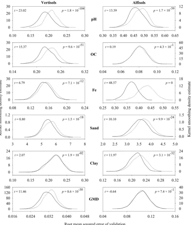
We further examined the statistical significance of the RMSE values of the best model (obtained by OPS approach) and that of full-spectrum model. A bootstrapping approach with replacement was repeated 1000 times to generate a distribution of RMSE values for each of these two models from the validation dataset.Fig. 3shows the kernel smoothing density estimates of the generated RMSE distributions of full-spectrum and best models for all soil attributes. Thisfigure shows that the mean RMSE values for the best models were generally less compared to their full-spectrum counterparts. A right-tail Student'st-test at 5% significance level (α= 0.05) was also used to compare the mean of RMSE values
observed from the bootstrapping approach. The Student'st-test showed that the mean of RMSE distribution of the best model was significantly lower than that of the full-spectrum model for all the soil attributes (pb0.05) except for OC (p= 0.43) and GMD (p= 0.74) in Alfisols. Both the best and full-spectrum model appeared to have similar predic-tion accuracy in case of OC and GMD in Alfisols. These results are consis-tent with the argument that a variable selection approach should allow one to build a regression model with fewer variables, which is capable of providing model performance either better than or, at least, equiva-lent to the original set of variables (Fernández Pierna et al., 2009).
Table 3lists the regression statistics of prediction of soil attributes using the best indicators in conjunction with OPS approach. Interestingly, the best models obtained with the OPS approach appeared to have better performance statistics in the validation dataset and somewhat reduced
Fig. 3.Distribution of root mean squared error of validation generated by bootstrapping for full-spectrum (dotted lines) and best (solid lines) models;tandpindicate thet-statistic and p-value of the Student'st-test, respectively.
statistics in the calibration datasets than those when full-spectrum was used for model development (Table 2). The reduction in model performance in calibration data may be attributed to the ability of OPS approach to reduce over-fitting of DRS models with the exclusion of less informative spectral variables. The significant improvement in the prediction accuracy noted for best models (compared to full-spectrum counterparts) advocates the use of OPS approach to develop efficient DRS models. The best models appeared to have the aforesaid advantages using a subset of spectral variables (as identified using the OPS ap-proach) from those used to build full-spectrum models (NSV = 2048). Specifically, the optimum NSV used to develop best models were less than or equal to 10% of NSV used in the full-spectrum model for Fe (4%), OC (4%), sand content (10%) in Alfisols, and sand content (9%), OC (10%) in Vertisols. For all the remaining soil attributes, the percentage of full-spectrum NSV varied between 12% (pH in Alfisols) and 49% (clay content in Vertisols). These results highlight the potential of OPS ap-proach in parsimonious representation of soil spectral reflectance.
In case of some soil attributes, it may be argued that a simple ap-proach of spectra data dimension reduction such as‘resampling’ spec-tral reflectance over 5 nm (NSV = 410) or 10 nm (NSV = 205) sampling intervals would yield low NSV than that achieved by implementing OPS approach. But the mean value of the RMSE distribu-tion in the validadistribu-tion of such models developed from resampled spectra was found to be significantly higher (α= 0.05) than those for best models for all the soil attributes except OC (5 nm resampling), GMD (both 5 and 10 nm resampling) in Vertisols and for OC (both 5 and 10 nm resampling) in Alfisols, as evaluated by implementing the boot-strap sampling in conjunction with Student'st-test approach detailed above (onlyfinal results are discussed).
The optimum spectral variables identified using best variable indica-tors for all soil attributes in both soil groups are presented inFig. 4. The electronic transitions due to Fe bearing minerals in the visible region (Sherman and Waite, 1985), thefirst overtone of O–H stretches and its combination with H–O–H bend around 1400 and 1900 nm (Clark, 1999) and the combination of metal–OH bend (around 2200 nm) asso-ciated with the clay mineral (Chabrillat et al., 2002; Viscarra Rossel et al., 2006) were found to be the most common optimum spectral variables across all the soil attributes. All the above wavelength regions are known for their significance in the estimation of soil attributes using DRS approach (Vohland et al., 2014); the OPS approach implemented in this study was successful in characterizing these features. This under-lines the potential of variable indicator-based OPS approach in making physically reasonable spectral variables selection (Teófilo et al., 2009).
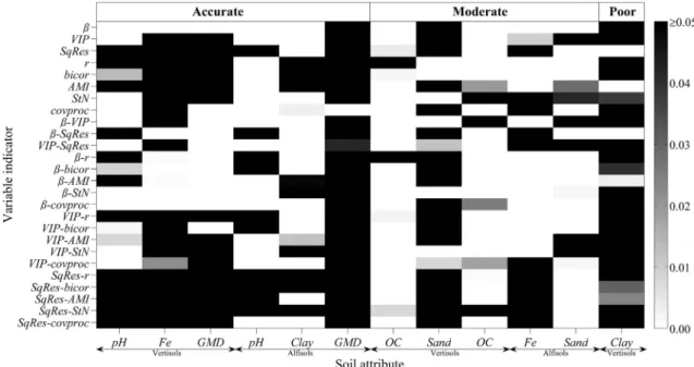
The OPS approach provided best variable indicators for each soil at-tribute in both Vertisols and Alfisols although it is desirable to have a general variable indicator irrespective of soil attribute or soil type. We assumed that the general variable indicator is the one which gives sig-nificant improvement in the prediction accuracy (compared to full-spectrum model) for majority of the soil attributes when used in con-junction with OPS approach. For this purpose, the bootstrapping ap-proach together with Student's t-test (detailed above) was implemented to generate and compare RMSE distribution in the valida-tion of all the optimum models inFig. 2with that of full-spectrum model. Thep-value of the test was used to judge the performance of op-timum models (Fig. 5). The frequency of success (pb0.05) of each opti-mum model across all the soil attributes was examined after classifying them based on their prediction accuracies (Table 2).Fig. 5shows that the indicators such asβ,CovProcandβ–CovProcare the most successful
Fig. 4.Optimum spectral variables selected using best variable indicator.β: regression coefficient,VIP: variable influence on projection,SqRes: squared residual vector,AMI: mutual information based adjacency vector,StN: signal to noise ratio,CovProc: covariance procedure. A hyphen between two individual variable indicators represents their pairwise combination.
variable indicators in case of accurately predicted soil attributes (5 out of 6 cases) whilebicorandβ–StNwere effective for all the moderately predicted soil attributes. Among these successful variable indicators, highest priority was given to PLSR-independent variable indicators as they are easy to compute and least uncertain compared to PLSR-dependent counterparts which are highly sensitive to the latent structure (Teófilo et al., 2009). Accordingly,CovProcandbicormay be regarded as the general variable indicators to be used with the OPS approach for accurate and moderate DRS models of soils, respectively.
4. Summary and conclusions
The selection of optimum spectral variables is an important step to improve robustness, accuracy and reduce complexity of DRS models. The OPS approach using variable indicators was found to be simple and accurate among several approaches implemented for optimum spectral variable selection. So far, the variable indicator-based wave-length selection has been cross-validated only withβas the variable indicator. The main objective of this study was to examine the utility of different PLSR-dependent (β, VIP, SqRes), PLSR-independent (r,bicor,AMI,StN,CovProc) and combined variable indicators in conjunction with OPS approach for optimum spectral variable selection. Efforts were also made to identify the best variable indicator for different soil attributes. The analyses were performed using pH, OC, Fe, sand content, clay content and GMD in two distinctly different soil groups of Vertisols and Alfisols of Karnataka, India. The PLSR models were evaluated using RPD of an independent validation dataset. Initially, a model with optimum NSV for each variable indicator was found by minimum-RMSE criteria. Then, the best variable indicator was selected based on both the accuracy (RMSE) and complexity (NSV) criteria with regard to the full-spectrum model. Accordingly,β(or its combinations) was found to be appropriate for Fe,CovProc(or its combinations) for pH,AMI(or its combinations) for clay content, andβ–SqResfor GMD in both Vertisols and Alfisols. An attempt was made to identify a general variable indicator for the practical utility of OPS approach. The variable indicators namely,CovProcandbicor were found to be more appropriate for accurate and moderate DRS models in this study, respectively. However, it may be noted that the variable indicators, which appeared to be inferior in this study, may be found more appropriate for some other dataset and, hence,
the variable selection approach warrants further investigation. The results of this study reaffirmed that the optimum spectral variables improve DRS model performance explicitly with the implementation of OPS approach. The overall results of the analyses advocated the use of PLSR-independent and their combination with PLSR-dependent vari-able indicators under OPS framework to develop simple and effective DRS models for soils.
Acknowledgments
The corresponding author gratefully acknowledges IIT Kharagpur for
financial support granted in the form of doctoral assistantship during measurements involved in this study. We are thankful to the Agricultural and Food Engineering Department, IIT Kharagpur in providing spectro-radiometer facility. We also thank the anonymous reviewers for their constructive comments.
References
Abdi, D., Tremblay, G.F., Ziadi, N., Bélanger, G., Parent, L.-É., 2012. Predicting soil phosphorus-related properties using near-infrared reflectance spectroscopy. Soil Sci. Soc. Am. J. 76, 2318–2326.http://dx.doi.org/10.2136/sssaj2012.0155.
Araújo, M.C.U., Saldanha, T.C.B., Galvão, R.K.H., Yoneyama, T., Chame, H.C., Visani, V., 2001. The successive projections algorithm for variable selection in spectroscopic multicomponent analysis. Chemom. Intell. Lab. Syst. 57, 65–73.http://dx.doi.org/ 10.1016/S0169-7439(01)00119-8.
Bayer, A., Bachmann, M., Müller, A., Kaufmann, H., 2012. A comparison of feature-based MLR and PLS regression techniques for the prediction of three soil constituents in a degraded South African ecosystem. Appl. Environ. Soil Sci. 2012, 1–20.http://dx.doi. org/10.1155/2012/971252.
Ben-Dor, E., Banin, A., 1995. Near-infrared analysis as a rapid method to simultaneously evaluate several soil properties. Soil Sci. Soc. Am. J. 59, 364–372.http://dx.doi.org/ 10.2136/sssaj1995.03615995005900020014x.
Brown, P.J., 1992. Wavelength selection in multicomponent near-infrared calibration. J. Chemom. 6, 151–161.http://dx.doi.org/10.1002/cem.1180060306.
Brown, D.J., Shepherd, K.D., Walsh, M.G., Dewayne Mays, M., Reinsch, T.G., 2006. Global soil characterization with VNIR diffuse reflectance spectroscopy. Geoderma 132, 273–290.http://dx.doi.org/10.1016/j.geoderma.2005.04.025.
Centner, V., Massart, D.L., de Noord, O.E., de Jong, S., Vandeginste, B.M., Sterna, C., 1996. Elimination of uninformative variables for multivariate calibration. Anal. Chem. 68, 3851–3858.http://dx.doi.org/10.1021/ac960321m.
Chabrillat, S., Goetz, A.F., Krosley, L., Olsen, H.W., 2002. Use of hyperspectral images in the identification and mapping of expansive clay soils and the role of spatial resolution. Remote Sens. Environ. 82, 431–445.http://dx.doi.org/10.1016/S0034-4257(02)00060-3. Fig. 5.Map ofp-value of Student'st-test between root mean squared error distributions in the validation of full-spectrum and optimum models.β: regression coefficient,VIP: variable influence on projection,SqRes: squared residual vector,r: Pearson correlation coefficients,bicor: biweightmidcorrelation vector,AMI: mutual information based adjacency vector,StN: sig-nal to noise ratio,CovProc: covariance procedure. A hyphen between two individual variable indicators represents their pairwise combination.
Chang, C.-W., Laird, D.A., Mausbach, M.J., Hurburgh, C.R., 2001. Near-infrared reflectance spectroscopy–principal components regression analyses of soil properties. Soil Sci. Soc. Am. J. 65, 480–490.http://dx.doi.org/10.2136/sssaj2001.652480x.
Chen, H., Pan, T., Chen, J., Lu, Q., 2011. Waveband selection for NIR spectroscopy analysis of soil organic matter based on SG smoothing and MWPLS methods. Chemom. Intell. Lab. Syst. 107, 139–146.http://dx.doi.org/10.1016/j.chemolab.2011.02.008. Clark, R.N., 1999.Spectroscopy of rocks and minerals, and principles of spectroscopy. In:
Rencz, A. (Ed.), Remote Sensing for the Earth Sciences: Manual of Remote Sensing. American Society for Photogrammetry and Remote Sensing, pp. 3–58.
Daniel, K.W., Tripathi, N.K., Honda, K., 2003. Artificial neural network analysis of laboratory and in situ spectra for the estimation of macronutrients in soils of Lop Buri (Thailand). Aust. J. Soil Res. 41, 47–59.http://dx.doi.org/10.1071/SR02027.
Fernández Pierna, J.A., Abbas, O., Baeten, V., Dardenne, P., 2009. A backward variable selection method for PLS regression (BVSPLS). Anal. Chim. Acta 642, 89–93.http:// dx.doi.org/10.1016/j.aca.2008.12.002.
Ferré, J., Faber, N.K.M, 2003. Net analyte signal calculation for multivariate calibration. Chemom. Intell. Lab. Syst. 69, 123–136. http://dx.doi.org/10.1016/S0169-7439(03)00118-7.
Ge, Y., Thomasson, J.A., 2006.Wavelet incorporated spectral analysis for soil property determination. Trans. ASABE 49, 1193–1201.
Gee, G.W., Bauder, J.W., 1986. Particle-size analysis. In: Klute, A. (Ed.), Methods of Soil Analysis. Part 1. Physical and Mineralogical Methods, SSSA Book Series. Soil Science Society of America, American Society of Agronomy, Madison, WI, pp. 383–412
http://dx.doi.org/10.2136/sssabookser5.1.2ed.c15.
Goldshleger, N., Chudnovsky, A., Ben-Dor, E., 2012. Using reflectance spectroscopy and artificial neural network to assess water infiltration rate into the soil profile. Appl. Environ. Soil Sci. 2012, 1–9.http://dx.doi.org/10.1155/2012/439567.
Jouan-Rimbaud, D., Walczak, B., Massart, D.L., Last, I.R., Prebble, K.A., 1995. Comparison of multivariate methods based on latent vectors and methods based on wavelength selection for the analysis of near-infrared spectroscopic data. Anal. Chim. Acta 304, 285–295.http://dx.doi.org/10.1016/0003-2670(94)00590-I.
Kinoshita, R., Moebius-Clune, B.N., van Es, H.M., Hively, W.D., Bilgilis, A.V., 2012. Strategies for soil quality assessment using visible and near-infrared reflectance spectroscopy in a western Kenya chronosequence. Soil Sci. Soc. Am. J. 76, 1776–1788.http://dx.doi.org/ 10.2136/sssaj2011.0307.
Kirkpatrick, S., Gelatt, C.D., Vecchi, M.P., 1983. Optimization by simulated annealing. Science 220, 671–680.http://dx.doi.org/10.1126/science.220.4598.671.
Leardi, R., Boggia, R., Terrile, M., 1992. Genetic algorithms as a strategy for feature selection. J. Chemom. 6, 267–281.http://dx.doi.org/10.1002/cem.1180060506.
Li, H., Liang, Y., Xu, Q., Cao, D., 2009. Key wavelengths screening using competitive adaptive reweighted sampling method for multivariate calibration. Anal. Chim. Acta 648, 77–84.
http://dx.doi.org/10.1016/j.aca.2009.06.046.
Lotse, E.G., Datta, N.P., Tomar, K.P., Motsara, K.P., 1972.Mineralogical composition of some red and black soils of India. Proc. Indian Nat. Sci. Acad.Springer, pp. 216–226
Morgan, C.L.S., Waiser, T.H., Brown, D.J., Hallmark, C.T., 2009. Simulated in situ characterization of soil organic and inorganic carbon with visible near-infrared diffuse reflectance spectroscopy. Geoderma 151, 249–256.http://dx.doi.org/10.1016/j. geoderma.2009.04.010.
Mosteller, F., Tukey, J.W., 1977.Data Analysis and Regression: A Second Course in Statistics. Addison Wesley, London.
Mouazen, A.M., Kuang, B., De Baerdemaeker, J., Ramon, H., 2010. Comparison among princi-pal component, partial least squares and back propagation neural network analyses for accuracy of measurement of selected soil properties with visible and near infrared spec-troscopy. Geoderma 158, 23–31.http://dx.doi.org/10.1016/j.geoderma.2010.03.001. Nadler, B., Coifman, R.R., 2005. The prediction error in CLS and PLS: the importance of feature
selection prior to multivariate calibration. J. Chemom. 19, 107–118.http://dx.doi.org/10. 1002/cem.915.
Norgaard, L., Saudland, A., Wagner, J., Nielsen, J.P., Munck, L., Engelsen, S.B., 2000. Interval partial least-squares regression (iPLS): a comparative chemometric study with an example from near-infrared spectroscopy. Appl. Spectrosc. 54, 413–419.http://dx.doi. org/10.1366/0003702001949500.
Reinikainen, S.-P., Hoskuldsson, A., 2003. COVPROC method: strategy in modeling dynamic systems. J. Chemom. 17, 130–139.http://dx.doi.org/10.1002/cem.770.
Sarathjith, M.C., Das, B.S., Vasava, H.B., Mohanty, B., Sahadevan, A.S., Wani, S.P., Sahrawat, K.L., 2014a. Diffuse reflectance spectroscopic approach for the characterization of soil aggregate size distribution. Soil Sci. Soc. Am. J. 78, 369–376.http://dx.doi.org/10.2136/ sssaj2013.08.0377.
Sarathjith, M.C., Das, B.S., Wani, S.P., Sahrawat, K.L., 2014b. Dependency measures for assessing the covariation of spectrally active and inactive soil properties in diffuse reflectance spectroscopy. Soil Sci. Soc. Am. J. 78, 1522–1530.http://dx.doi.org/10. 2136/sssaj2014.04.0173.
Shepherd, K.D., Walsh, M.G., 2002.Development of reflectance spectral libraries for characterization of soil properties. Soil Sci. Soc. Am. J. 66, 988–998.
Sherman, D., Waite, T., 1985.Electronic spectra of Fe (super 3 +) oxides and oxide hydroxides in the near IR to near UV. Am. Mineral. 70, 1262–1269.
Song, L., Langfelder, P., Horvath, S., 2012. Comparison of co-expression measures: mutual information, correlation, and model based indices. BMC Bioinf. 13, 328.http://dx.doi. org/10.1186/1471-2105-13-328.
Soriano-Disla, J.M., Janik, L.J., Viscarra Rossel, R.A., Macdonald, L.M., McLaughlin, M.J., 2014. The performance of visible, near-, and mid-infrared reflectance spectroscopy for prediction of soil physical, chemical, and biological properties. Appl. Spectrosc. Rev. 49, 139–186.http://dx.doi.org/10.1080/05704928.2013.811081.
Stenberg, B., Rossel, R.A.V., Mouazen, A.M., Wetterlind, J., 2010. Visible and near infrared spectroscopy in soil science. In: Sparks, D.L. (Ed.), Advances in Agronomy. Academic Press, Burlington, pp. 163–215http://dx.doi.org/10.1016/S0065-2113(10)07005-7. Stevens, A., van Wesemael, B., Vandenschrick, G., Touré, S., Tychon, B., 2006. Detection of
carbon stock change in agricultural soils using spectroscopic techniques. Soil Sci. Soc. Am. J. 70, 844–850.http://dx.doi.org/10.2136/sssaj2005.0025.
Tekin, Y., Tumsavas, Z., Mouazen, A.M., 2012. Effect of moisture content on prediction of organic carbon and pH using visible and near-infrared spectroscopy. Soil Sci. Soc. Am. J. 76, 188–198.http://dx.doi.org/10.2136/sssaj2011.0021.
Teófilo, R.F., Martins, J.P.A., Ferreira, M.M.C., 2009. Sorting variables by using informative vectors as a strategy for feature selection in multivariate regression. J. Chemom. 23, 32–48.http://dx.doi.org/10.1002/cem.1192.
Thissen, U., Ustün, B., Melssen, W.J., Buydens, L.M.C., 2004. Multivariate calibration with least-squares support vector machines. Anal. Chem. 76, 3099–3105.http://dx.doi. org/10.1021/ac035522m.
Vasques, G.M., Grunwald, S., Harris, W.G., 2009a. Spectroscopic models of soil organic carbon in Florida, USA. J. Environ. Qual. 39, 923–934.http://dx.doi.org/10.2134/ jeq2009.0314.
Vasques, G.M., Grunwald, S., Sickman, J.O., 2009b. Modeling of soil organic carbon fractions using visible–near-infrared spectroscopy. Soil Sci. Soc. Am. J. 73, 176–184.
http://dx.doi.org/10.2136/sssaj2008.0015.
Viscarra Rossel, R., 2007. Robust modelling of soil diffuse reflectance spectra by bagging-partial least squares regression. J. Near Infrared Spectrosc. 15, 39–47.http://dx.doi.org/ 10.1255/jnirs.694.
Viscarra Rossel, R.A., Lark, R.M., 2009. Improved analysis and modelling of soil diffuse reflectance spectra using wavelets. Eur. J. Soil Sci. 60, 453–464.http://dx.doi.org/10. 1111/j.1365-2389.2009.01121.x.
Viscarra Rossel, R.A., Webster, R., 2012. Predicting soil properties from the Australian soil visible-near infrared spectroscopic database. Eur. J. Soil Sci. 63, 848–860.http://dx. doi.org/10.1111/j.1365-2389.2012.01495.x.
Viscarra Rossel, R.A., Walvoort, D.J.J., McBratney, A.B., Janik, L.J., Skjemstad, J.O., 2006. Visible, near infrared, mid infrared or combined diffuse reflectance spectroscopy for simulta-neous assessment of various soil properties. Geoderma 131, 59–75.http://dx.doi.org/ 10.1016/j.geoderma.2005.03.007.
Vohland, M., Ludwig, M., Thiele-Bruhn, S., Ludwig, B., 2014. Determination of soil properties with visible to near- and mid-infrared spectroscopy: effects of spectral variable selec-tion. Geoderma 223-225, 88–96.http://dx.doi.org/10.1016/j.geoderma.2014.01.013. Walkley, A., Black, I.A., 1934. An examination of the Degtjareff method for determining soil
organic matter, and a proposed modification of the chromic acid titration method. Soil Sci. 37, 29–38.http://dx.doi.org/10.1097/00010694-193401000-00003. Wilcox, R., 2005.Introduction to Robust Estimation and Hypothesis Testing. second ed.
Elsevier, Amsterdam.
Wold, S., Johansson, E., Cocchi, M., 1993.PLS—partial least squares projections to latent structures. In: Kubinyi, H. (Ed.), 3D QSAR in Drug Design. ESCOM Science, Leiden, pp. 523–548.
Xiaobo, Z., Jiewen, Z., Povey, M.J.W., Holmes, M., Hanpin, M., 2010. Variables selection methods in near-infrared spectroscopy. Anal. Chim. Acta 667, 14–32.http://dx.doi. org/10.1016/j.aca.2010.03.048.