DETERMINANTS OF FISCAL DECENTRALIZATION: POLITICAL ECONOMY
ASPECTS
Mario Jametti, Marcelin Joanis
Document de treball de l’IEB
2010/7
Documents de Treball de l’IEB 2010/7
DETERMINANTS OF FISCAL DECENTRALIZATION:
POLITICAL ECONOMY ASPECTS
Mario Jametti, Marcelin Joanis
The
IEB
research program in
Fiscal Federalism
aims at promoting research in the public
finance issues that arise in decentralized countries. Special emphasis is put on applied
research and on work that tries to shed light on policy-design issues. Research that is
particularly policy-relevant from a Spanish perspective is given special consideration.
Disseminating research findings to a broader audience is also an aim of the program. The
program enjoys the support from the
IEB-Foundation
and the
IEB-UB
Chair in Fiscal
Federalism funded by Fundación ICO, Instituto de Estudios Fiscales and Institut d’Estudis
Autonòmics.
The
Barcelona Institute of Economics (IEB)
is a research centre at the University of
Barcelona which specializes in the field of applied economics. Through the
IEB-Foundation
, several private institutions (Caixa Catalunya, Abertis, La Caixa, Gas Natural
and Applus) support several research programs.
Postal Address:
Institut d’Economia de Barcelona
Facultat d’Economia i Empresa
Universitat de Barcelona
C/ Tinent Coronel Valenzuela, 1-11
(08034) Barcelona, Spain
Tel.: + 34 93 403 46 46
Fax: + 34 93 403 98 32
ieb@ub.edu
http://www.ieb.ub.edu
The IEB working papers represent ongoing research that is circulated to encourage
discussion and has not undergone a peer review process. Any opinions expressed here are
those of the author(s) and not those of IEB.
Documents de Treball de l’IEB 2010/7
DETERMINANTS OF FISCAL DECENTRALIZATION:
POLITICAL ECONOMY ASPECTS
*Mario Jametti, Marcelin Joanis
ABSTRACT:
This paper empirically investigates the underlying causes of expenditure
decentralization, based on the predictions of a new political economy model of partial fiscal
decentralization. Under shared expenditure responsibility, the degree of decentralization is
endogenous and depends on the relative political conditions prevailing at each level of
government. Our empirical results from a panel of democracies support the relevance of
political factors as determinants of fiscal decentralization. The relationship between central
government electoral strength and both expenditure and revenue centralization emerges as
nontrivial and non-linear. Political forces at the central government level driving
centralization up and down appear to coexist.
JEL Codes: H77, D72, H11
Keywords: fiscal decentralization, fiscal federalism, vertical interactions, partial
decentralization, elections.
Mario Jametti
Institute for Microeconomics and Public
Economics (MecoP)
University of Lugano
Via G. Bu¢ 6,
6904 Lugano, Switzerland
E-mail: mario.jametti@lu.unisi.ch
Marcelin Joanis
Department of Economics
Université de Sherbrooke
Faculté d’administration,
2500 boul. de l’Université
Sherbrooke (Québec), Canada, J1K 2R1
E-mail: marcelin.joanis@usherbrooke.ca
*
We wish to thank Bob Inman for insightful comments, and Youri Chassin for his help with data collection. Financial support from the Institut d’Economia de Barcelona (IEB) is greatfully acknowledged. The responsibility for any error remains ours.
1
Introduction
Sub-central governments enjoy larger degrees of competence in revenue and expenditure deci-sions, a trend that has been documented empirically (Arzaghi and Henderson, 2005). What are the determinants of this trend? And what are the channels through which decentralization is achieved? These questions, while on top of the policy agenda, have been relatively little explored.
In this paper we point to two directions we consider relevant in understanding the mecha-nisms of delegation of competencies to lower level governments: …rst, in many instances there is joint contribution and shared responsibility in the provision of speci…c public goods by two or more levels of government. This implies that we need to adapt our theoretical framework by moving away from considering decentralization as a binary choice –i.e. provisioneither by the central or lower level government, as generally assumed in the …scal federalism literature – and toward explicitly taking into account the interplay arising from joint provision. Hence, decentralization is often of partial nature. Second, politics matters: we argue that the degree of decentralization within a country depends in important ways on the relative political forces between levels of government.
Most of the theoretical literature in economics treats the decision to decentralize as a binary one. Based on the “Decentralization Theorem” (Oates, 1972) allocation of public goods and services is guided by a trade-o¤ between internalizing inter-jurisdictional spillovers and catering to local preferences.1 Notably, even what is known as the Second Generation Theory of Fiscal Federalism (Weingast, 2009), while moving away from assuming benevolent governments2 to include political dimensions, still essentially remains within a binary choice framework.
1
See Epple and Nechyba (2004) for a recent survey.
Conversely, actual decentralization policies generally imply overlap in spending duties by two or more levels of government. Breton (1996) argues that few countries do indeed have a fully centralized government structure. Even unitary states, such as France and Spain, have lower level authorities, often with elected o¢ cials.
We de…ne partial decentralization as a situation where a public good is provided by more than one level of government. Jametti and Joanis (2009a) using raw data from the IMF’s Gov-ernment Financial Statistics show that even within fairly disaggregate spending items, such as education, health and culture, there is contribution from three levels of government (central, state and local) in Canada, Switzerland and the U.S. Similarly, within their database, consid-ering between 40 and 50 countries with at least some (overall) expenditure decentralization and the aforementioned spending items, only cultural spending in India is fully decentralized. Partial decentralization gives rise to vertical interactions among governments on two dimen-sions. First, complementarities in spending among levels of government make joint contribution socially optimal. Second, vertical externalities arise among politicians as they might bene…t and react strategically to the contribution to the public good of another level of government.
The latter dimension is the main focus of this paper, the political economy of partial decentralization having received relatively little attention in the literature.3 Our analysis is based on an earlier paper by Joanis (2009), which is cast in the context of a pure moral hazard political agency model, an approach initiated by Barro (1973) and Ferejohn (1986). In the model, two levels of government are involved in the provision of a public good and voters are imperfectly informed about each government’s contribution to the good, creating a shared accountability problem. An important feature of the model is that the degree of decentralization
3
We are aware of two recent exceptions: Brueckner (2009) studies partial …scal decentralization in a Tiebout-style framework, while Hat…eld and Padro i Miquel’s (2008) analysis is cast in a tax competition framework. Neither of these papers provide an empirical application.
is endogenous in the model and depends on three elements: (i) the relative competence of each level of government, (ii) the relative rents that politicians at each level of government can earn from holding o¢ ce, captured in the model by each level of government’s access to the tax base, and (iii) the relative political conditions prevailing at each level of government, i.e. the extent to which each level of government can a¤ect its electoral fortunes by contributing to the public good.
This paper’s focus is on the third of these predictions, with the theory’s main insight being that the central government’s electoral strength should, all else being equal, increase that government’s share of spending. Using data from a panel of democracies, we explore the role of electoral conditions prevailing at the central level on the degree of both expenditure and revenue centralization. Fixed e¤ects regressions generally support the theory, together with highlighting the non-linear nature of the empirical relationship between centralization and government strength. Overall, these results show that electoral variables rightly belong in the set of determinants of …scal decentralization.
The paper proceeds as follows. After a brief discussion of the related empirical literature in Section 2, Section 3 lays down the theoretical model and derives empirically-testable pre-dictions. Section 4 introduces the empirical strategy and describes the data, with empirical results being presented in Section 5. The last section concludes brie‡y.
2
Contribution to the Literature
This paper is related to the large body of empirical research investigating decentralization as a determinant of various economic variables, where decentralization is measured in terms of a revenue or expenditure ratio between di¤erent levels of government, e.g. sub-federal divided
by total government expenditures. For example, Oates (1985) relates the size of government to the degree of decentralization, a question that has been taken up by a number of studies (for a survey, see Feld et al., 2003). Thus, decentralization often features as an explanatory variable in empirical research on …scal federalism.
Much smaller – but closer to our purpose – is the empirical literature on the actual de-terminants of …scal decentralization. An early, cross-sectional attempt is Panizza (1999), who …nds that country size, income, ethnic fractionalization and the degree of democracy all reduce the degree of …scal decentralization. Similar results are presented by Arzaghi and Henderson (2005), using panel data. A more recent study, also in a panel context, on the determinants of decentralization in Switzerland (Feld et al., 2008) shows that centralization is negatively related to the availability of direct democratic decision-making (referenda). Stegarescu (2009) documents the role of political integration as a determinant of …scal decentralization in OECD countries.
We expand the existing literature on the determinants of …scal decentralization along three dimensions: First, as mentioned above, in most of the theoretical literature, the devolution of public good provision and …nancing is assumed to be a binary decision, e.g. expenditures are either provided by the central or the local government. Second, political economy aspects of decentralization are generally introduced in an ad hoc way in the empirical analysis.4 Our analysis is based on a theoretical political economy framework, thus introducing explicitly the e¤ects of political choices on the degree of decentralization. Third, we see a better modeling of the determinants of decentralization as a stepping stone towards addressing the issues that arise in models where decentralization is used as an explanatory variable –such as the “Oates” regressions from above –which su¤er quite obviously from endogeneity problems. In particular,
4Panizza (1999) does present a theoretical model in which the degree of centralization is endogenously
the potential for endogeneity problems is evident in the theoretical model presented in the next section, in which the degree of decentralization is an equilibrium outcome. Our work can be seen as an exploration of potential instruments for decentralization variables in other applications.
3
A Model of Shared Responsibility in a Federation
This section lays down a model in which a public good valued by the voters in a given juris-diction is jointly provided by two levels of government (labelled ‘federal’and ‘provincial’). It describes the environment (composed of two governments andN identical voters), characterizes the social optimum, and derives key results on the political determinants of decentralization.5 In each of two periods, two levels of government choose …scal policy (taxes collected and spending) to maximize their expected level of rent extraction, subject to the constraint that they need to seek reelection at the end of the …rst period. Voters, who value public goods, can observe total taxes and can infer total rents. However, they do not observe the intergovernmen-tal composition of expenditures. Public good provision is positively related to the reelection probability of both governments such that the spending decisions of one level of government a¤ects not only its own reelection probability but that of the other level of government as well (a positive externality arises). Each level of government’s equilibrium contribution to the public good equates its own marginal bene…t from reelection – with an incentive to free-ride on the other level of government’s contribution –to the marginal cost of foregone rents in the …rst period, taking as given the strategy of the other level of government.
5
3.1 The Environment
Every period, the federal government (indexed by superscriptf) and the provincial government (indexed by superscript p) each contribute to the provision of a public good g in a province. Government j produces gj 0 units of a publicly-provided input. Together, the federal and provincial inputs are converted into a public good g by a constant elasticity of substitution (CES) technology:6
g= f(gf) + p(gp) 1= ; (1)
where 1: p and f are parameters that denote each level of government’s competence. Each government levies a lump-sum tax (Tj) and faces a common unit cost of produc-tion (~). Politicians in o¢ ce can divert tax revenues away from public good provision and towards their own bene…t. Assuming balanced budgets at each level of government, any of the jurisdiction’sN individuals faces a total tax bill of
T =Tf+Tp= (gf +gp) +sf +sp; (2)
where = ~=N and sj are the per capita rents extracted by governmentj. All individuals have the following quasi-linear utility function:
u(g; z) =h(g) +z; (3)
wherez denotes the consumption of a private good and h is a well-behaved concave function.
6
For tractability, let us assume a simple functional form forh:
h(g) =g ; (4)
where 0 < < 1. Furthermore, every period each individual is endowed with y units of the private good such that
z+T =y: (5)
Without loss of generality, we normalize the population of the jurisdiction to unity (N = 1) since all individuals are identical.
For simplicity, let us make a few additional assumptions about taxes. Since taxes are lump-sum in this model, we can aslump-sume that individuals and governments take total taxes collected (Tp and Tf) as given. Let us further assume thatTp andTf are …xed at some pre-determined
levels that are su¢ cient for each level of government to provide some arbitrary maximum level of the public good (g). In sum, we assume the following series of inequalities for each governmentj:
g Tj y: (6)
3.2 Benevolent Governments and the Optimal Degree of Decentralization
Given our focus on the extent of decentralization on the expenditure side, for expositional purposes, it will be useful to de…ne the ‘degree of decentralization’(d) as the share of provincial spending in total spending:
d g
p
The case in which d = 1 will be referred to as complete decentralization, d = 0 as complete centralization, and0< d <1will correspond to instances ofpartial decentralization.
Optimality requires that politicians extract no rents while in o¢ ce (sf S = spS = 0) and that the Samuelson condition be satis…ed (a superscript S denotes the social optimum). In this model, the latter implies that government j contributes to the public good according to the following expression:
gjS= 1 1 ( j)11 ( j) 1 1 + ( j) 1 1 ( 1) if <1; (8)
where jdenotes the other level of government. It follows from (8) that the optimal spending ratio (which determines the optimal degree of decentralization) is a function of the relative competence of the two levels of government:
gp gf S = p f 1 1 : (9)
If the inputs produced by both levels of government do not exhibit any complementarity ( = 1) – a case in which these inputs are ‘perfect substitutes’– the socially optimal levels of gf and
gp are given by the following conditions:
gjS = 1 j 1 1 if j > j; gp+gf = 1 1 1 if p= f = ;for some ; gjS = 0 if j < j: (10)
Proposition 1 (Optimal Decentralization) The involvement of both levels of government in the provision of a public good – i.e. ‘partial decentralization’– is optimal provided that there is some degree of complementarity between gf and gp:Complete centralization can be optimal only if there is no complementarity in gf andgp ( = 1) and if the federal government is more
competent than the provincial government ( f p). Similarly, complete decentralization is optimal only if = 1 and f p:
In what follows, we assume that <1.
3.3 Introducing Politics: Opportunistic Politicians and Strategic Voters
Unless governments are assumed to be benevolent social planners, their behaviour depends on the incentives provided by the political process. This paper considers a two-period model, with separate elections taking place at the provincial and federal levels between the two periods. As in Besley and Smart’s (2006, 2007) political agency model, elections in our model can act as an imperfect disciplinary device.
Politicians Each government maximizes expected discounted rents (per capita) over the two
periods, given by
Sj =sj1+Pj sj2; (11)
where subscripts indicate periods, 2 [0;1] is a discount factor and Pj is incumbent j’s perception of his reelection probability.
Voters and elections Voters face a simple binary reelection decision in the elections held
place simultaneously.7 Furthermore, following Besley and Smart (2006), voters are taken to be able to announce and commit to a reelection rule before the elections take place.
Information The information available to voters at election time is crucial to the ability of
elections to act as disciplinary devices. Two sources of imperfect information will be crucial to the analysis that follows:
1. Voters do not observe the contribution of each level of government to the shared public good. However, voters observe the aggregate level of the public good. In other words, voters observe gbut notgf andgp.
2. Uncertainty about the election outcome is introduced and resolved only after incumbents have taken all relevant decisions and just before the voters cast their ballots. From the point of view of incumbents, elections are ‘probabilistic.’
In the spirit of probabilistic voting models, such as those developed by Persson and Tabellini (2000) or more recently by Alesina and Tabellini (2007, 2008), election results are typically uncertain from the point of view of politicians (at least to some extent) since a series of shocks may a¤ect the electorate’s decision beyond …scal policy (e.g. other issues arising during the campaign, characteristics of challengers, partisan loyalty). Here, these shocks are speci…c to a given level of government, introducing heterogeneity in the electoral conditions between the elections taking place at the two levels of government.
Timing The timing of the game is as follows:
1. Incumbents set period-1 …scal policy (determining the contribution to the shared public good and the level of rents);
2. Voters observe the realization of two random variables which summarize the electoral conditions speci…c to each election;
3. The federal and provincial elections take place; and
4. If reelected, the incumbents set period-2 …scal policy. Otherwise, voters achieve the utility level associated with challengers (similar in all respects to incumbents).
3.4 Equilibrium and predictions
Voters announce that they will reelect each incumbent if their period-1 utility level exceeds some random threshold value,8 the distribution of which is assumed to be common knowledge. The cut-o¤ utility level relevant to the provincial election is denoteduand is a random variable distributed according toF;a c.d.f. Hence, voters reelect the provincial government if
u(g; T) u: (12)
Symmetrically, they reelect the federal government is their utility exceeds the realization of a random variablev; distributed according toG; a c.d.f.
From the point of view of incumbents, reelection is probabilistic. Electoral results depend on aggregate public good provision and on the realization of the stochastic reservation utility levels. The probability that the provincial incumbent is reelected is
Pp = Pr [u(g; T) u] =F[u(g; T)]: (13)
For simplicity, let us assume that u is uniformly distributed on the interval [0; u ], implying
8One interpretation for this is that information about the quality of the challengers becomes available just
that
Pp= 1
u u(g; T): (14)
Note that the reelection probability is decreasing inu , the upper bound on the random cut-o¤ utility level. Hence, the election is riskier from the incumbent’s point of view the higher is this upper bound.
We can now consider the provincial incumbent’s problem in period 1:
max gp T
p gp+ Tp 1
u (
f(gf) + p(gp) ) = Tp Tf ; (15)
which is obtained by substituting the government’s budget constraint ( gp +sp = Tp) and equation (14) in equation (11).9 The federal government solves a symmetric problem, with
v U[0; v ]:The two levels of government are assumed to behave non-cooperatively in setting their contribution to the public good, taking the contribution level of the other government as given. Since elections are simultaneous, the equilibrium contribution levels in period 1 will be those observed in a Nash equilibrium.
Under shared responsibility, the degree of decentralization is endogenous and is the outcome of vertical interactions between the two levels of government that are shaped by the degree of substitutability between the public inputs.10 The reaction functions are given by:
Tp u ( f(gf) + p(gp) ) 1 (gp) 1 p = ; (16) Tf v ( f(gf) + p(gp) ) 1 (gf) 1 f = : (17) 9
Time subscripts are dropped from now on since the period-2 problem is trivial, with maximum rents being taken by each government. All decision variables relate to period 1.
1 0
Whereas high complementarity mitigates the ability of each government to merely free-ride on the other’s contribution, complementarity is also associated with a more indirect e¤ect of aggregate spending on reelection probabilities.
Solving (16) for an interior solution yields the Nash equilibrium spending ratio: gp gf = p f Tp Tf v u 1 1 ; (18)
which in general is di¤erent from the optimal spending ratio given by equation (9), unless
Tpv =Tfu :
Proposition 2 (Endogenous decentralization) The equilibrium degree of decentralization
corresponds to the optimal degree of decentralization only if TTfp =
u
v ;i.e. if the provincial-federal
revenue ratio is equal to the provincial-federal ratio of the voters’ reservation utility levels. Otherwise, the equilibrium spending ratio di¤ ers from the optimal ratio and is determined by the product of three ratios: the relative competencies pf , the revenue ratio
Tp
Tf , and the
relative reelection uncertainties vu .
Hence, a decentralization reform that leads to de facto shared expenditure responsibilities may not be socially optimal despite the existence of complementarities amongst levels of gov-ernment. The key reasons for why this is the case in this model are (i) voters’inability to hold each level of government individually liable for its actions, and (ii) vertical interactions among levels of government, which take into account factors other than relative competencies.
The theoretical model thus leads to the following empirically-relevant equation:
gp gf =f p f; Tp Tf; v u +"; (19)
where "is an error term. In the remainder of this paper, we develop an empirical implemen-tation of this equation. Our main endeavour is to identify the e¤ect of electoral conditions on the observed degree of decentralization.
4
Empirical Framework and Data
Equation (18) implies a relationship between the degree of expenditure decentralization and three ratios:
1. Relative competencies: This ratio captures a technological advantage of one level of
government over the other. For example, in the spirit of Oates’ decentralization the-orem, if f < p; that is the level of government closest to citizens has an advantage in production, equilibrium (and optimal) expenditure decentralization will favour the provincial government. While this ratio is interesting in its own right, we will assume in the following empirical application that it does not vary within country over time. As a consequence, its e¤ect will be captured by the country …xed e¤ects.
2. Revenue ratio: Not surprisingly, the model predicts that expenditure decentralization
is closely related to how the tax base is split between the two levels of government. To avoid obvious endogeneity issues in including the revenue ratio among our right-hand side variables, our preferred empirical speci…cations will exclude the revenue ratio. However, revenue decentralization is interesting in its own right, and we investigate its determinants in the next section.
3. Relative reelection uncertainties: This is our main ratio of interest. Recall that
u and v capture the uncertainty of the election at each level of government. When
v increases, the reelection prospects of the federal incumbent become more uncertain. Ceteris paribus, this reduces the incumbent’s incentive to spend on the public good. The same is true at the subcentral level. However, in what follows, because of a lack of electoral data at the subcentral level we will assume that while v varies within country over time, u does not.
For the purpose of our empirical analysis we assembled a new database combining informa-tion from four sources: the IMF’s Government Financial Statistics (GFS); the World Bank’s Dataset of Political Indicators (DPI) and World Development Indicators (WDI); and the Polity 2 dataset from the University of Maryland. Country data is at the annual level. We dispose of an unbalanced panel of a total of 107 countries for the period 1990 to 2006.11
From GFS we included data on expenditures and revenues of di¤erent levels of government (central, state and local). We have used this information to construct our measures of central-ization (or decentralcentral-ization). DPI contains information on the political system of each country as well as a vast array of electoral variables, such as party composition and strength of national governments and oppositions. We used this information for our measures of political strength. The WDI dataset gives variables concerning overall economic indicators and constitutes our basis for additional control variables. Finally, the primary use of Polity 2 is to restrict our sample to democracies.
Our dependent variables correspond to centralization ratios:
CEN T RAL= g
c
gc+gs+gl; (20)
where g is government expenditure (or revenues); c is central government; s is state or sub-federal government; andlis local government. Thus, we contrast central government decisions with decisions taken at any sub-central unit. Data is taken from the GFS-Series 2 “Cash expen-diture”for central, state and local governments.12 We exclude observations with centralization
1 1
Not all countries present data for all years. A total of 104 countries present at least one year of central government expenditure. The countries formed out of Yugoslavia are considered individually in our dataset. Note that our dataset includes all the countries of Panizza (1999) except: Central African Republic, Guatemala, Honduras, Iraq, Jordan, Kenya, Malawi, New Zealand, Senegal, Sri Lanka, Yemen and Zaire.
1 2We computed overall public expenditure as indicated in (20). GFS contains the government unit “General
Government”, which, in principle should correspond to the denominator of (20). However, information on this variable is lacking in many instances, and hence we did not use it. Additionally, we have run our regressions
ratios equal to one, since we are unable to distinguish between absence of sub-central spending and missing data.13
The political variables that we include in our analysis intend to capture the absolute strength of the government, the relative strength vis-à-vis the opposition and the dispersion of opposition political forces. To capture government strength (GOVSTREN), we use …ve political variables:
Central Government Seat Share (M AJ): Share of seats held by the government.14
Central Government Vote Share (N U M V OT E): Share of votes held by the
govern-ment. Depending on the electoral system (e.g. the …rst-past-the-post system in Canada)
N U M V OT E can be di¤erent from the seat distribution (M AJ).
Central Government Seat Advantage (SEAT ADV): The di¤erence between
legis-lature seats held by government (N U M GOV) and by opposition (N U M OP P) as a ratio of total seats. Total seats is de…ned as the sum of government, opposition and unaligned
(N U M U L) seats. Note that seat advantage can be negative.
Central Government Her…ndahl Index (HERF GOV): Sum of squared seat shares
of government parties.
Central Opposition Her…ndahl Index (HERF OP P): Sum of squared seat shares
of opposition parties.
Seat share and vote share of the government represent the absolute political strength of the government; seat advantage captures the relative strength of the government compared to
using the Series 7 “Outlays”. Results do not vary signi…cantly and are available upon request.
1 3
Inspection of the data showed that the expenditure centralization ratio in Romania for 1990 was less than 1%. We dropped this observation as well.
its opposition; government Her…ndahl Index (HHI) is an indication of the political spectrum that is combined within the government parties, a government is likely to be weaker if it has to rely on coalitions with a large number of parties holding di¤erent views. Finally, opposition HHI is an indicator of the political dispersion of opposition parties. A high HHI is an indicator of a fragmented opposition, hence potentially more leeway for the government. All political variables are taken directly from DPI, except central government seat advantage which we constructed.15 Additionally, we include in all our regressions the logs of GDP per capita, pop-ulation and poppop-ulation density, all taken from WDI. They form theX vector in the regression equation (below).
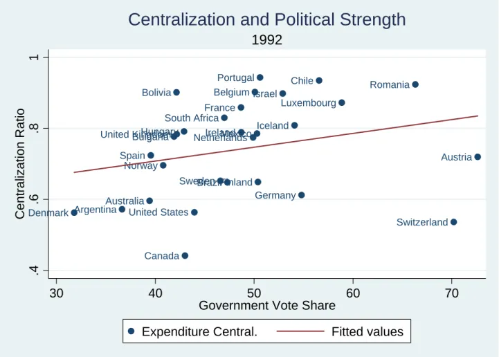
Figure 1 presents a scatterplot of the centralization ratio and the central government vote share for the year 1992. We observe a slightly positive raw correlation, indicating that higher political strength seems to favour higher centralization ratios, consistent with the theoretical model’s prediction. Table 1 presents summary statistics of our dataset.
In order to move beyond such unconditional correlations, regression results follow in the next section.
5
Estimation and Results
We implement the following linear version of equation (19):
CEN T RALjt = + GOVSTRENjt+ Xjt+COUNTRYj +YEARt+"jt; (21)
1 5
We excluded observations where government vote share was equal to zero (N U M V OT E= 0). Note that the number of observations with missing values varies across the di¤erent political variables, which implies that the sample varies across speci…cations.
whereCOUNTRYj is a vector of country …xed e¤ects, andYEARtis a vector of year e¤ects.
We ran panel data least squares regressions including country …xed e¤ects and year e¤ects in all our speci…cations. A constant is always included, though unreported.
5.1 Base Regressions
Table 2 presents our baseline expenditure speci…cations. We present results using the seat share, vote share and seat advantage variables in turn, while we include, besides the additional controls, the opposition HHI in all speci…cations. Further, some speci…cations allow for possibly non-linear e¤ects including squares and cubes of the government strength variables.16 Standard errors are robust.
Our sample contains between 453 and 530 observations, from 59 to 64 countries. The dif-ferent speci…cations explain between 18% and 46% of total variation, and the economic control variables are all highly signi…cant and in line with expectations. Higher income and higher population density increase expenditure centralization, while a larger population decreases it. A …rst important result is that in all our speci…cations the political variables included are jointly highly signi…cant, as illustrated by the Wald-test statistic in the last two rows of the table.17 Columns (1) to (3) of Table 2 present the results using seat share (M AJ) to represent the political strength of the government. In a linear speci…cation, column (1) suggests that a higher seat share leads toless centralization (more decentralization). The negative coe¢ cient on the M AJ variable thus appears to contradict the raw correlation of Figure 1. However, columns (2) and (3) suggest that this relationship is likely to be non-linear. Including the square of M AJ reveals the expected positive linear term, with a negative square term (both
1 6
In support for the latter functional forms, note the nonlinear form of equation (18). We come back to the nonlinearity issue in our discussion of the results below.
1 7
In this subsection, inference is based on robust standard errors. See the next subsection for a discussion of clustering issues.
are statistically signi…cant). Finally, we obtain the best results statistically when we also include a cubic term of M AJ, where all coe¢ cients are signi…cant at the 1% level. Again, signs of the coe¢ cients switch, this time with a negative linear, positive square and negative cubic term. We …nd similar results using the government vote share (columns (4) to (6)).
Using seat advantage to measure relative political strength (columns (7) to (9)) seems to stand on slightly weaker statistical grounds. Only the squared term is signi…cant (at the 5% level) if allowing for linear and square terms, while only the square and cubic ones are signi…cant if allowing for all three terms. Finally, in column (10) we include the government HHI as a political variable but do not …nd any signi…cant e¤ect. The opposition HHI is included in all ten speci…cations, and is negative and signi…cant in three of them. Hence, a stronger opposition (as measured by a larger concentration index) tends to imply lower levels of centralization. This is in line with the theory’s prediction that a weak central government should be associated with more decentralization.
Table 3 presents the same speci…cations using revenue centralization as the dependent variable. As for the expenditure regressions, the political variables are jointly signi…cant in all speci…cations. Furthermore, the coe¢ cient on the opposition HHI is now highly signi…cantly negative in all speci…cations. The estimated patterns for the government strength variables are similar to those estimated in expenditure speci…cations, again highlighting the nonlinear nature of the relationship.
5.2 Robustness Checks
As a robustness check we present, in Table 4, the results of our most ‡exible speci…cations (using cubic terms) with clustered standard errors at the country level. Indeed, as shown by Stock and Watson (2008), the heteroskedasticity robust standard errors following White
(1980), commonly used, may be signi…cantly biased in a panel context. They suggest, among other, the use of clustered standard errors, where the clusters are applied at the dimension of the …xed e¤ect.18 The results of Stock and Watson (2008) depend on …xed T and it has been reported that the clustering method might be unstable in situations of unbalanced panels (see Nichols and Scha¤er, 2007).
As expected, our results with clustered standard errors are slightly more conservative. Nev-ertheless, the included political variables are jointly signi…cant at the 5% level in all regressions. Individual coe¢ cients for seat shares (M AJ), both for expenditures and revenues and govern-ment vote share (N U M V OT E), only for expenditures are still signi…cant at conventional levels.
5.3 Discussion of Results
What do our results imply? Our main result is that political variables are important determi-nants of the degree of centralization. However, all of our empirical results do not necessarily con…rm our priors. On the one hand, results based on the opposition Her…ndhal index suggest that a strong central government tends to be associated with more centralization. But on the other hand, looking at Table 1 we observe that in the linear speci…cation (column (1)) political strength of the federal government, measured by the government seat share, has a negative impact on the degree of centralization. Hence, our proxy of lower (federal) reelection uncer-tainty fails to predict an increase in the contribution to the federal public good. This result is robust when we allow for the most ‡exible parameterization. Figure 2 presents the e¤ect of government seat share in the cubic speci…cation on the degree of centralization, showing a
1 8
Indeed, as of Version 10, Stata automatically presents the clustered standard errors when using the option “robust”.
consistently signi…cant negative impact, at least over the range of centralization we observe.19 Figure 2 also nicely illustrates the nonlinearity of the relationship between government strength and centralization. In particular, there appears to be a di¤erential e¤ect towards the bounds of the domain (0 and 1). Although corner solutions were intentionally left out of the theoretical discussion to simplify exposition, nonlinear outcomes are likely to arise in the model because reelection probabilities are bounded – see equation (14) above. For a given government, the incentive to spend more to improve reelection prospects disappears when the reelection probability hits one. A similar issue may arise at the zero bound.
But besides highlighting the nonlinear nature of the relationship, our mixed empirical results suggest that our simple theoretical model does not fully capture the complexity of government behaviour. Should a strong government ‘invest’ more in public good provision when its re-election prospects are higher? The implicit assumption in our model is yes: when rere-election uncertainty decreases, public spending is a safer investment for the incumbent. This view of government behaviour is consistent with a theoretical perspective, due to Cox and McCubbins (1986) and revisited in Joanis (forthcoming), for which the latter …nd strong empirical support in a distributive politics application. However, a competing view of government behaviour, in the Downsian tradition, predicts that an incumbent should be expected to spend more when the election is highly uncertain –see, for example, Lindbeck and Weibull (1987). In our context, this “swing voter”view of government incentives would predict an activist central government when its reelection prospects areuncertain. In line with the discussion in Joanis (forthcoming), a more complete theoretical model would nest both views of government behaviour, which have both been shown to be empirically relevant.
1 9
Con…dence intervals are calculated based on clustered standard errors, consistent with the previous subsec-tion.
6
Conclusion
All levels of government in a federation (or a decentralized ‘unitary’ state) are more or less involved in similar sectors of activity. In such a context – typical in real-world federations – making coherent collective choices is a complex undertaking for voters, who need to garner information about the contribution of each level of government to the aggregate policy out-comes that they observe. To capture such informational complexity, this paper has considered a political agency model in which the presence of a hierarchy of governments involved in the provision of a public good creates an externality on the spending side (with respect to the intergovernmental composition of government spending). In the model, the provision of public goods by both levels of government in a federation is the margin along which political compe-tition occurs. In a given subnational jurisdiction, the central and the subnational governments compete for the support of the same voters (though in separate elections) by each providing public goods. Under some realistic conditions –chie‡y, imperfectly informed voters and substi-tutable central and subnational public goods –the model predicts that the equilibrium degree of decentralization will diverge from the social optimum.
Our empirical results lend support to that theoretical perspective. They support the rele-vance of political factors as determinants of …scal decentralization. The empirical application of this paper has focused on one aspect of the political economy of …scal decentralization, that is the in‡uence of central government electoral strength. The relationship between the latter and both expenditure and revenue centralization emerges as nontrivial and nonlinear. Political forces driving centralization down –the linear e¤ect of seat and vote shares –and up –the e¤ect of opposition composition –appear to coexist (see our discussion in the previous subsection).
im-proved along many dimensions. Our dataset presents a number of important issues that pre-clude us from estimating our model the way we wish. First, since we do not observe sub-central political outcomes, we cannot use information on the relative strength of government. Second, our data cover general spending only. More precise results might be obtained using speci…c spending categories, more in line with our theoretical model. Despite these drawbacks, we think that our analysis is a useful …rst step into assessing the e¤ect of political instances on the issue of …scal decentralization.
But further work is obviously needed to re…ne those early results. This paper is part of a broader, ongoing research agenda. In future work, we intend to test the predictions of the Joanis (2009) theoretical model in a broad set of institutional environments. We are currently conducting similar empirical studies with a panel of Canadian provinces (Jametti and Joanis, 2009b) and a panel of Swiss cantons, in which it is possible to include subnational elections data in the analysis. An interesting avenue would be to explicitly include the ‘relative competencies’ in the empirical analysis, perhaps using Public Sector E¢ ciency (PSE) measures – see, for example, Afonsoet al. (2005).
Despite these necessary re…nements, the analysis already has interesting implications for policy design, highlighting the need for decentralization reforms to take into account the real-ity of the political process. For example, shared responsibilreal-ity in policy areas that are politi-cally sensitive (e.g. infrastructure investment) may be especially conducive to ine¢ cient public spending. With partial decentralization of expenditure responsibilities being an increasingly pervasive institution in both developed and developing countries, this paper indicates a need to shift the policy focus from whether decentralization is desirable to how decentralization is actually implemented.
References
[1] Afonso, Antonio, Ludger Schuknecht and Vito Tanzi (2005). Public Sector E¢ ciency: an International Comparison,Public Choice, 123, 321-347.
[2] Alesina, Alberto and Guido Tabellini (2007). “Bureaucrats or Politicians? Part I: A Single Policy Task,”American Economic Review, 97, 169-179.
[3] Alesina, Alberto and Guido Tabellini (2008). “Bureaucrats or Politicians? Part II: Multiple Policy Tasks,”Journal of Public Economics, 92, no. 3-4, 426-447.
[4] Arzaghi, Mohammad and J. Vernon Henderson (2005). “Why Countries are Fiscally De-centralizing?”Journal of Public Economics, 89, 1157-1189.
[5] Barro, Robert (1973). “The Control of Politicians: An Economic Model,”Public Choice, 14, 19-42.
[6] Besley, Timothy and Michael Smart (2006). “Political Agency and Public Finance,” pp. 174-227 in: Timothy Besley (ed.), Principled Agents? The Political Economy of Good Government, Oxford University Press: Oxford.
[7] Besley, Timothy and Michael Smart (2007). “Fiscal Restraint and Voter Welfare,”Journal of Public Economics, 91, 755-773.
[8] Breton, Albert (1996). Competitive Governments: An Economic Theory of Politics and Public Finance, Cambridge: Cambridge University Press.
[9] Brueckner, Jan K. (2009). “Partial …scal decentralization,”Regional Science and Urban Economics, 39(1), 23-32, January.
[10] Cox, Gary W. and Mathew D. McCubbins (1986). “Electoral politics as a distributive game,”Journal of Politics, 48, no. 2, 370-389.
[11] Epple, Dennis and Thomas Nechyba (2004). “Fiscal Decentralization,” in J. Vernon Hen-derson and Jacques-Françcois Thisse (Eds.),Handbook of Regional and Urban Economics Vol 4 - Cities and Geography, Elsevier - North Holland.
[12] Feld, Lars P., Gebhard Kirchgässner and Christoph A. Schaltegger (2003). “Decentralized Taxation and the Size of Government: Evidence from Swiss State and Local Governments,” CESifo working paper 1087.
[13] Feld, Lars P., Christoph A. Schaltegger and Jan Schnellenbach (2008). “On Government Centralization and Fiscal Referendums,”European Economic Review, 52, 611-645.
[14] Ferejohn, John (1986). “Incumbent Performance and Electoral Control,”Public Choice, 50, 5-25.
[15] Hat…eld, John William and Gerard Padro i Miquel (2008). “A Political Economy Theory of Partial Decentralization,” NBER Working Papers 14628.
[16] Jametti, Mario and Marcelin Joanis (2009a). “The Rise of Partial Decentralization and Shared Responsibility Federalism,” mimeo.
[17] Jametti, Mario and Marcelin Joanis (2009b). “The Political Economy of Fiscal Decentral-ization: Evidence from the Canadian Federation,” mimeo.
[18] Joanis, Marcelin (2009). “Intertwined Federalism: Accountability Problems under Partial Decentralization,” CIRANO working paper 2009-s39.
[19] Joanis, Marcelin (forthcoming). “The Road to Power: Partisan Loyalty and the Central-ized Provision of Local Infrastructure,”Public Choice.
[20] Lindbeck, Assar and Jörgen W. Weibull (1987). “Balanced-budget redistribution as the outcome of political competition,”Public Choice, 52(3), 273-297.
[21] Nichols, Austin and Mark Scha¤er (2007). “Clustered Errors in Stata,” United Kingdom Stata Users’Group Meeting 2007.
[22] Nishimura, Yukihiro (2006). “Human Fallibility, Complementarity, and Fiscal Decentral-ization,"Journal of Public Economic Theory, 8(3), 487-501.
[23] Oates, Wallace E. (1972).Fiscal Federalism, New York: Harcourt Brace.
[24] Oates, Wallace E. (1985). “Searching for Leviathan: An Empirical Study,”American Economic Review, 75, 748-757.
[25] Oates, Wallace E. (2003). “Toward a Second-Generation Theory of Fiscal Federalism,” International Tax and Public Finance, 12, 349-373.
[26] Panizza, Ugo (1999). “On the Determinants of Fiscal Centralization: Theory and Evi-dence,”Journal of Public Economics, 74, 97-139.
[27] Persson, Torsten and Guido Tabellini (2000). Political Economics: Explaining Economic Policy, Cambridge: MIT Press.
[28] Stegarescu, Dan (2009). “The e¤ects of economic and political integration on …scal de-centralization: evidence from OECD countries,”Canadian Journal of Economics, 42(2), 694-718.
[29] Stock, James H. and Mark W. Watson (2008). “Heteroskedasticity-Robust Standard Errors for Fixed E¤ects Panel Data Regression,”Econometrica, 76(1), 155-174.
[30] Weingast, Barry R. (2009). “Second Generation Fiscal Federalism: The Implications of Fiscal Incentives,”Journal of Urban Economics, 65, 279-293.
[31] White, Halbert (1980). “A Heteroskedasticity-Consistent Covariance Matrix Estimator and a Direct Test for Heteroskedasticity,”Econometrica, 48, 817-838.
Figure 1
ArgentinaAustralia Austria Belgium Bolivia Brazil Bulgaria Canada Chile Denmark Finland France Germany Hungary Ireland IcelandIsrael Luxembourg Mexico Netherlands Norway Portugal Romania South Africa Spain Sweden Switzerland United Kingdom United States
.4
.6
.8
1
Centralization Ratio
30
40
50
60
70
Government Vote Share
Expenditure Central.
Fitted values
1992
Figure 2
-.6 -.4 -.2 0 0 .2 .4 .6 .8 1Central Government Seat Share
Effect on Centralization lower bound 95% CI upper bound 95% CI
Seat Share Cube
Variable Observations Mean Std. Dev. Min Max
Expenditure Centralization 558 0.77 0.14 0.40 0.99
Revenue Centralization 563 0.74 0.15 0.39 0.99
Central government seat share (MAJ) 802 0.60 0.18 0.11 1.00
Central government vote share (NUMVOTE) (in %) 665 50.70 15.77 5.50 100.00
Central government seat advantage (SEATADV) 802 0.21 0.35 ‐0.78 1.00
Central government Herfindahl index (HERFGOV) 798 0.69 0.29 0.01 1.00
Central opposition Herfindahl index (HERFOPP) 742 0.52 0.25 0.07 1.00
GDP per capita (constant 2000 US$) 557 10321.26 10549.92 129.20 38407.11
Population (in millions) 557 52.68 159.29 0.25 1079.72
Population Density 557 115.52 146.77 1.39 1254.06
Sources: GFS, DPI, WDI
Table 1 Summary Statistics
Dependent Variable = Ratio of Expenditure
Centralization (1) (2) (3) (4) (5) (6) (7) (8) (9) (10)
Central government seat share (MAJ) ‐0.04746** 0.22167*‐1.37754*** 0.01993 0.11577 0.37079
MAJ2 ‐0.22106** 2.53209***
0.09884 0.66304
MAJ3 ‐1.48522***
0.37983
Central government vote share (NUMVOTE) ‐0.00072** 0.00246** ‐0.01107*** 0.00029 0.00099 0.0023
NUMVOTE2 ‐0.00003*** 0.00023***
0.00001 0.00005
NUMVOTE3 ‐0.00000***
0
Central government seat advantage (SEATADV) ‐0.02412** ‐0.00156 0.01748 0.01013 0.0118 0.01267 SEATADV2 ‐0.05198** 0.07102** 0.0241 0.02894 SEATADV3 ‐0.17382*** 0.04688
Central government Herfindahl index (HERFGOV) 0.01193 0.00949 Central opposition Herfindahl index (HERFOPP) ‐0.02011* ‐0.01943 ‐0.02261* ‐0.00126 ‐0.00719 ‐0.01063 ‐0.01939 ‐0.0198 ‐0.02234* ‐0.01119
0.0118 0.01203 0.01217 0.0129 0.01274 0.01218 0.01183 0.01204 0.01229 0.01261
Log(GDP per capita) 0.08126*** 0.06926*** 0.05926*** 0.03003 0.02748 0.01367 0.08038*** 0.07041*** 0.05937*** 0.07950***
0.02304 0.02252 0.02218 0.02607 0.02613 0.02459 0.02287 0.02248 0.0222 0.02351 Log(Population) ‐2.06490***‐2.02158*** ‐1.58090**‐1.96732***‐1.76227*** ‐1.56251** ‐2.08411***‐2.00165***‐1.65759***‐2.11261*** 0.56895 0.54829 0.64241 0.56337 0.54712 0.66951 0.57056 0.55072 0.63926 0.60064 Log(Population Density) 1.92334*** 1.88509*** 1.43940** 1.57536*** 1.41742** 1.23732* 1.94346*** 1.86372*** 1.51807** 1.97726*** 0.57492 0.55551 0.64868 0.57456 0.56043 0.68107 0.57658 0.55819 0.64581 0.60349 Log likelihood 1220.97259 1227.62659 1242.7616 1083.24288 1095.45998 1117.46761 1221.08118 1227.16828 1240.25974 1217.79318 R‐squared 0.1957 0.21564 0.25918 0.37731 0.41 0.46463 0.19602 0.21428 0.25215 0.17739 Number of Observations 530 530 530 453 453 453 530 530 530 531 Number of Countries 64 64 64 59 59 59 64 64 64 64
Joint Significance of Political Variables 5.68 4.53 5.27 3.42 4.04 8.51 5.72 4.47 5.07 2.51 P‐value 0.0037 0.0039 0.0004 0.0339 0.0075 0.0000 0.0035 0.0042 0.0005 0.0827 * p<0.1, ** p<0.05, *** p<0.01
Notes: A constant, time effects and country fixed effects included in all regressions. Robust standard errors in italics.
Table 2
Dependent Variable = Ratio of Revenue
Centralization (1) (2) (3) (4) (5) (6) (7) (8) (9) (10)
Central government seat share (MAJ) ‐0.02863 0.20789*‐1.00224*** 0.02017 0.12239 0.37099 MAJ2 ‐0.19421* 1.88978*** 0.10217 0.66904 MAJ3 ‐1.12441*** 0.38362
Central government vote share (NUMVOTE) ‐0.0005 0.00354***‐0.00777*** 0.00031 0.00101 0.00289
NUMVOTE2 ‐0.00004*** 0.00018***
0.00001 0.00006
NUMVOTE3 ‐0.00000***
0
Central government seat advantage (SEATADV) ‐0.01359 0.00722 0.02187 0.01028 0.01364 0.01473
SEATADV2 ‐0.04787* 0.0459
0.02532 0.03125
SEATADV3 ‐0.13263***
0.04885
Central government Herfindahl index (HERFGOV) 0.01245 0.00974 Central opposition Herfindahl index (HERFOPP) ‐0.04049***‐0.03989***‐0.04234***‐0.04682***‐0.05452***‐0.05746***‐0.03999***‐0.04038***‐0.04236*** ‐0.03151**
0.01429 0.0145 0.01481 0.01448 0.01412 0.01381 0.01433 0.01461 0.01492 0.01483
Log(GDP per capita) 0.09487*** 0.08429*** 0.07664*** 0.07215** 0.06895** 0.05733** 0.09429*** 0.08507*** 0.07659*** 0.09368***
0.02939 0.02905 0.02862 0.02822 0.0271 0.02554 0.02928 0.02895 0.0286 0.02898 Log(Population) ‐2.37052***‐2.33108***‐1.99474***‐2.20797***‐1.94450*** ‐1.77461** ‐2.37175***‐2.29443***‐2.02940***‐2.53083*** 0.68071 0.64173 0.73664 0.68564 0.64263 0.79306 0.68353 0.64823 0.7347 0.6759 Log(Population Density) 2.12339*** 2.08855*** 1.74880** 1.79809** 1.59531** 1.44229* 2.12519*** 2.05052*** 1.78466** 2.29009*** 0.69142 0.65368 0.74631 0.69513 0.65428 0.80118 0.69419 0.66012 0.74445 0.68376 Log likelihood 1178.64569 1183.23179 1190.82406 1036.14818 1053.34367 1066.70412 1178.39436 1183.00436 1189.69424 1179.67722 R‐squared 0.22971 0.24308 0.2647 0.3416 0.39036 0.42573 0.22897 0.24242 0.26152 0.22481 Number of Observations 524 524 524 447 447 447 524 524 524 525 Number of Countries 64 64 64 59 59 59 64 64 64 64
Joint Significance of Political Variables 6.14 4.46 4.06 8.05 9.35 9.77 6.03 4.36 3.87 6.43 P‐value 0.0023 0.0042 0.0031 0.0004 0.0000 0.0000 0.0026 0.0048 0.0042 0.0018 * p<0.1, ** p<0.05, *** p<0.01
Notes: A constant, time effects and country fixed effects included in all regressions. Robust standard errors in italics.
Table 3
Dependent Variable =
(1) (2) (3) (4) (5) (6)
Central government seat share (MAJ) ‐1.37754** ‐1.00224*
0.57166 0.58724
MAJ2 2.53209** 1.88978*
1.05293 1.10442
MAJ3 ‐1.48522** ‐1.12441*
0.6239 0.66003
Central government vote share (NUMVOTE) ‐0.01107*** ‐0.00777**
0.00254 0.00374
NUMVOTE2 0.00023*** 0.00018**
0.00005 0.00007
NUMVOTE3 ‐0.00000*** ‐0.00000***
0.00000 0.00000
Central government seat advantage (SEATADV) 0.01748 0.02187
0.02058 0.02182
SEATADV2 0.07102 0.0459
0.0431 0.04496
SEATADV3 ‐0.17382** ‐0.13263
0.07668 0.08381
Central opposition Herfindahl index (HERFOPP) ‐0.02261 ‐0.01063 ‐0.02234 ‐0.04234** ‐0.05746*** ‐0.04236**
0.01453 0.0141 0.01477 0.01884 0.01716 0.01862
Log(GDP per capita) 0.05926* 0.01367 0.05937* 0.07664** 0.05733 0.07659**
0.03228 0.03589 0.03218 0.03656 0.0379 0.03619 Log(Population) ‐1.58090*** ‐1.56251*** ‐1.65759*** ‐1.99474*** ‐1.77461*** ‐2.02940*** 0.51506 0.53258 0.52382 0.63777 0.51291 0.62448 Log(Population Density) 1.43940** 1.23732** 1.51807** 1.74880** 1.44229** 1.78466*** 0.57144 0.57372 0.57875 0.68444 0.56615 0.67056 Log likelihood 1242.76 1117.47 1240.26 1190.82 1066.70 1189.69 R‐squared 0.26 0.46 0.25 0.26 0.43 0.26 Number of Observations 530 453 530 524 447 524 Number of Countries 64 59 64 64 59 64
Joint Significance of Political Variables 2.60 19.45 2.68 1.87 10.46 1.84
P‐value 0.0447 0.0000 0.0397 0.1268 0.0000 0.1318
* p<0.1, ** p<0.05, *** p<0.01
Notes: A constant, time effects and country fixed effects included in all regressions. Clustered (by country) standard errors in italics.
Expenditure Centralization Revenue Centralization Table 4
Documents de Treball de l’IEB
2007
2007/1. Durán Cabré, J.Mª.; Esteller Moré, A.: "An empirical analysis of wealth taxation: Equity vs. tax compliance"
2007/2. Jofre-Monseny, J.; Solé-Ollé, A.: "Tax differentials and agglomeration economies in intraregional firm location"
2007/3. Duch, N.; Montolio, D.; Mediavilla, M.: "Evaluating the impact of public subsidies on a firm’s performance: A quasi experimental approach"
2007/4. Sánchez Hugalde, A.: "Influencia de la inmigración en la elección escolar"
2007/5. Solé-Ollé, A.; Viladecans-Marsal, E.: "Economic and political determinants of urban expansion: Exploring the local connection"
2007/6. Segarra-Blasco, A.; García-Quevedo, J.; Teruel-Carrizosa, M.: "Barriers to innovation and public policy in Catalonia"
2007/7. Calero, J.; Escardíbul, J.O.: "Evaluación de servicios educativos: El rendimiento en los centros públicos y privados medido en PISA-2003"
2007/8. Argilés, J.M.; Duch Brown, N.: "A comparison of the economic and environmental performances of conventional and organic farming: Evidence from financial statement"
2008
2008/1. Castells, P.; Trillas, F.: "Political parties and the economy: Macro convergence, micro partisanship?"
2008/2. Solé-Ollé, A.; Sorribas-Navarro, P.: "Does partisan alignment affect the electoral reward of intergovernmental transfers?"
2008/3. Schelker, M.; Eichenberger, R.: "Rethinking public auditing institutions: Empirical evidence from Swiss municipalities"
2008/4. Jofre-Monseny, J.; Solé-Ollé, A.: "Which communities should be afraid of mobility? The effects of agglomeration economies on the sensitivity of firm location to local taxes"
2008/5. Duch-Brown, N.; García-Quevedo, J.; Montolio, D.: "Assessing the assignation of public subsidies: do the experts choose the most efficient R&D projects?"
2008/6. Solé-Ollé, A.; Hortas Rico, M.: "Does urban sprawl increase the costs of providing local public services? Evidence from Spanish municipalities"
2008/7. Sanromà, E.; Ramos, R.; Simón, H.: "Portabilidad del capital humano y asimilación de los inmigrantes. Evidencia para España"
2008/8. Trillas, F.: "Regulatory federalism in network industries"
2009
2009/1. Rork, J.C.; Wagner, G.A.: "Reciprocity and competition: is there a connection?"
2009/2. Mork, E.; Sjögren, A.; Svaleryd, H.: "Cheaper child care, more children"
2009/3. Rodden, J.: "Federalism and inter-regional redistribution"
2009/4. Ruggeri, G.C.: "Regional fiscal flows: measurement tools"
2009/5. Wrede, M.: "Agglomeration, tax competition, and fiscal equalization"
2009/6. Jametti, M.; von Ungern-Sternberg, T.: "Risk selection in natural disaster insurance"
2009/7. Solé-Ollé, A; Sorribas-Navarro, P.: "The dynamic adjustment of local government budgets: does Spain behave differently?"
2009/8. Sanromá, E.; Ramos, R.; Simón, H.: "Immigration wages in the Spanish Labour Market: Does the origin of human capital matter?"
2009/9. Mohnen, P.; Lokshin, B.: "What does it take for and R&D incentive policy to be effective?"
2009/10. Solé-Ollé, A.; Salinas, P..: "Evaluating the effects of decentralization on educational outcomes in Spain?"
2009/11. Libman, A.; Feld, L.P.: "Strategic Tax Collection and Fiscal Decentralization: The case of Russia"
2009/12. Falck, O.; Fritsch, M.; Heblich, S.: "Bohemians, human capital, and regional economic growth"
2009/13. Barrio-Castro, T.; García-Quevedo, J.: "The determinants of university patenting: do incentives matter?"
2009/14.Schmidheiny, K.; Brülhart, M.: "On the equivalence of location choice models: conditional logit, nested logit and poisson"
2009/15. Itaya, J., Okamuraz, M., Yamaguchix, C.: "Partial tax coordination in a repeated game setting"
2009/16. Ens, P.: "Tax competition and equalization: the impact of voluntary cooperation on the efficiency goal"
2009/17. Geys, B., Revelli, F.: "Decentralization, competition and the local tax mix: evidence from Flanders"
2009/18. Konrad, K., Kovenock, D.: "Competition for fdi with vintage investment and agglomeration advantages"
Documents de Treball de l’IEB
2009/20. Akai, N., Sato, M.: "Soft budgets and local borrowing regulation in a dynamic decentralized leadership model with saving and free mobility"
2009/21. Buzzacchi, L., Turati, G.: "Collective risks in local administrations: can a private insurer be better than a public mutual fund?"
2009/22. Jarkko, H.: "Voluntary pension savings: the effects of the finnish tax reform on savers’ behaviour"
2009/23. Fehr, H.; Kindermann, F.: "Pension funding and individual accounts in economies with life-cyclers and myopes"
2009/24. Esteller-Moré, A.; Rizzo, L.: "(Uncontrolled) Aggregate shocks or vertical tax interdependence? Evidence from gasoline and cigarettes"
2009/25. Goodspeed, T.; Haughwout, A.: "On the optimal design of disaster insurance in a federation"
2009/26. Porto, E.; Revelli, F.: "Central command, local hazard and the race to the top"
2009/27. Piolatto, A.: "Plurality versus proportional electoral rule: study of voters’ representativeness"
2009/28. Roeder, K.: "Optimal taxes and pensions in a society with myopic agents"
2009/29, Porcelli, F.: "Effects of fiscal decentralisation and electoral accountability on government efficiency evidence from the Italian health care sector"
2009/30, Troumpounis, O.: "Suggesting an alternative electoral proportional system. Blank votes count"
2009/31, Mejer, M., Pottelsberghe de la Potterie, B.: "Economic incongruities in the European patent system"
2009/32, Solé-Ollé, A.: "Inter-regional redistribution through infrastructure investment: tactical or programmatic?"
2009/33, Joanis, M.: "Sharing the blame? Local electoral accountability and centralized school finance in California"
2009/34, Parcero, O.J.: "Optimal country’s policy towards multinationals when local regions can choose between firm-specific and non-firm-specific policies"
2009/35, Cordero, J,M.; Pedraja, F.; Salinas, J.: "Efficiency measurement in the Spanish cadastral units through DEA"
2009/36, Fiva, J.; Natvik, G.J.: "Do re-election probabilities influence public investment?"
2009/37, Haupt, A.; Krieger, T.: "The role of mobility in tax and subsidy competition"
2009/38, Viladecans-Marsal, E; Arauzo-Carod, J.M.: "Can a knowledge-based cluster be created? The case of the Barcelona 22@district"
2010
2010/1, De Borger, B., Pauwels, W.: "A Nash bargaining solution to models of tax and investment competition: tolls and investment in serial transport corridors"
2010/2, Chirinko, R.; Wilson, D.: "Can Lower Tax Rates Be Bought? Business Rent-Seeking And Tax Competition Among U.S. States"
2010/3, Esteller-Moré, A.; Rizzo, L.: "Politics or mobility? Evidence from us excise taxation"
2010/4, Roehrs, S.; Stadelmann, D.: "Mobility and local income redistribution"
2010/5, Fernández Llera, R.; García Valiñas, M.A.: "Efficiency and elusion: both sides of public enterprises in Spain"
2010/6, González Alegre, J.: "Fiscal decentralization and intergovernmental grants: the European regional policy and Spanish autonomous regions"