NBER WORKING PAPER SERIES
DOES GROWING INEQUALITY REDUCE TAX PROGRESSIVITY? SHOULD IT?
Joel Slemrod Jon Bakija
Working Paper7576
http://www.nber.org/papers/w7576
NATIONAL BUREAU OF ECONOMIC RESEARCH 1050 Massachusetts Avenue
Cambridge, MA 02138 March 2000
Prepared for the American Enterprise Institute conference on "The Role of Inequality in Tax Policy," January 21-2, 1999, Washington, D.C. We are grateful for helpful comments from Jim Poterba, Bill Gale, and other participants in the AEI conference and at a presentation of the paper at the Georgetown Law Center. The views expressed herein are those of the authors and are not necessarily those of the National Bureau of Economic Research.
© 2000 by Joel Slemrod and Jon Bakija. All rights reserved. Short sections of text, not to exceed two paragraphs, may be quoted without explicit permission provided that full credit, including © notice, is given to the source.
Does Growing Inequality Reduce Tax Progressivity? Should It?
Joel Slemrod and Jon Bakija NBER Working Paper No. 7576 March 2000
JEL No. H2
ABSTRACT
This paper explores the links between two phenomena of the past two decades: striking increase in the inequality of pre-tax incomes, and the failure of tax-and-transfer progressivity to increase. We emphasize the causal links going from inequality to progressivity, noting that optimal taxation theory predicts that growing inequality should increase progressivity. We discuss public choice alternatives to the optimal progressivity framework. The paper also addresses the opposite causal direction: that it is changes in taxation that have caused an apparent increase in inequality. Finally, we discuss the “non-event-study” offered by the large changes in the distribution of income--with no major tax changes-- since 1995, and discuss its implications for the link between progressivity and inequality.
Joel Slemrod Jon Bakija
University of Michigan Business School Williams College
701 Tappan Street, Room A2120 Williamstown, MA 01267 Ann Arbor, MI 48109-1234
and NBER
Does Growing Inequality Reduce Tax Progressivity? Should It? Joel Slemrod and Jon Bakija
1. Introduction
Over at least the past two decades the average real income of the bottom four deciles has stagnated, while the real income of those at the top of the income distribution has grown sharply. Income inequality has sharply increased.
During the same period, the progressivity of the tax-and-transfer system has not increased, and has arguably declined. In the decade of the 1980’s the progressivity of the federal tax system first declined, and then increased, so that in 1990 it was not
substantially different from what it was in 1980.1 Arguably, the top rate increases of 1990 and 1993 increased progressivity, but the expansion of capital gains tax preferences in 1997 and, possibly after, offset the higher top rates. The generosity of transfers to the poor has declined, too.
This paper explores the links between these two phenomena. We emphasize the causal link going from inequality to progressivity, noting that optimal taxation theory predicts the opposite of what has occurred -- that growing inequality should increase
1 The Congressional Budget Office has calculated a consistent series of tax distribution for about two decades. This series uses a definition of income somewhat broader than adjusted gross income, includes all federal taxes, and assumes that the burden of the corporate income tax falls on capital income generally. Under these assumptions, the average tax rate on the top 1 percent of income earners fell from 34.9 percent to 26.2 percent between 1980 and 1985, rose to 36.5 percent by 1995, and then fell slightly to 34.4. percent by 1999. Average tax rates were changed very little between 1980 and 1999 for most of the rest of the income distribution. The average rate on the second lowest quintile fell slightly from 15.0 percent to 13.7 percent between 1980 and 1999. In the middle quintile, the average rate edged down from 19.1 percent to 18.9 percent. In the second highest quintile, the average rate was 22.2 percent in both 1980 and 1999. The rate for the top quintile went from 28.2 percent to 29.1 percent. The bottom quintile did experience a substantial decline in average federal tax rates, from 7.7 percent to 4.6 percent, largely due to an increased personal exemption and standard deduction after 1986, and expansion of the earned income tax credit. However, this does not take into account reductions in transfers such as food stamps and welfare payments. The combined tax and transfer system is thus probably not much different in its progressivity in 1999 than it was in 1980. Source: Kasten, Sammartino, and Toder (1994), and Congressional Budget Office (1998c).
progressivity. We discuss public choice alternatives to the optimal progressivity
framework. The paper also addresses the opposite causal direction -- that it is changes in taxation that have caused the (apparent) increase in inequality -- and also the possibility that the two phenomena are causally unrelated, but caused by a common set of exogenous factors.
In Section 6, we make two empirical contributions to this debate. First, we argue that standard measures of income distribution ignore the implications of the large recent run-up in stock prices, and attempt a crude calculation of what this impact might be. We calculate the distribution of income taking account of the stock market runup, and
compare it to more standard measures that ignore it. In addition, the effective tax rate on these gains is arguably quite low, reducing the progressivity of the tax system much below what standard measures suggest. Finally, we investigate the “non-event study” offered by the large changes in the distribution of income beginning in 1996, and discuss its implications for the issues addressed by this paper.
2. Should Increased Inequality Reduce Tax Progressivity? 2.1 Optimal Progressivity Theory
The modern theory of optimal progressivity accepts, for the sake of argument, the right of government to redistribute income through the tax system (and other means), sidesteps the ethical arguments about the value of a more equal distribution of economic outcomes, and instead investigates the implications of various value judgments and parameters of the economic system for the design of the tax system. Front and center comes the fact that greater redistribution of income requires higher marginal tax rates, which may provide disincentives to work, save, take risks, and invest in human and
physical capital. The essential problem, then, is to describe the inherent tradeoffs between the distribution of income and economic performance.
Mirrlees (1971) initiated the modern literature formalizing this tradeoff. In his formulation, the government must choose an income tax schedule to raise a given amount of total revenue, with the goal of maximizing a utilitarian social welfare function. This function implicitly trades off the welfare of individuals at different income levels, but assumes that social welfare increases when any member of society (including the richest) is better off, holding others’ welfare constant. It therefore precludes envy as the basis of tax policy.2 Mirrlees first investigated what characterizes the optimal income tax3 for any set of assumptions about the social welfare function, the distribution of endowments, and the behavioral response (utility) functions. He concluded that in this general case only very weak conditions characterize the optimal tax structure, conditions that offer little concrete guidance in the construction of a tax schedule.
In the absence of general results, the approach has been to make specific
assumptions about the key elements of the model, and then to calculate the parameters of the optimal income tax system. This approach is meant to suggest the characteristics of the optimal income tax under reasonable assumptions and to investigate how these characteristics depend on the elements of the model. Mirrlees also pioneered this approach in his 1971 article, and concluded that the optimal tax structure is
approximately linear (that is, it has a constant marginal tax rate and an exemption level below which tax liability is negative) and has marginal tax rates which were quite low by then current standards, usually between 20 and 30 percent and almost always less than 40
2 Feldstein (1976) offers an excellent review of these issues.
3 Because a tax schedule may feature rebates rather than taxes at some levels of income, it is really the optimal tax-and-transfer system that is at issue in the optimal progressivity literature.
percent.4 This was a stunning and unexpected result even, it seems, to Mirrlees himself, and especially in an era where top rates of 70 percent or more were the norm.
Subsequent work investigated the sensitivity of the optimal income tax to the parametric assumptions. Of particular interest to the topic at hand, Mirrlees presented an example in which widening the distribution of skills, assumed equal to wage rates, increased the optimal marginal tax rates, though he considered the dispersion of skills necessary to imply much higher rates to be unrealistic. In his baseline numerical simulation he set the value of σ (the standard deviation of the associated normal
distribution) in the assumed logarithmal distribution of skills to be equal to 0.39, derived from Lydall’s (1968) figures for the distribution of income from employment for various countries. When Mirrlees repeats the simulation with σ=1.0, a much wider dispersion of ability, he reports (p. 207) that the optimal tax schedule
is in almost all respects very different. Tax rates are very high: a large proportion of the population is allowed to abstain from productive labour. The results seem to say that, in an economy with more intrinsic inequality in economic skill, the income tax is a more important weapon of public control than it is in an economy where the dispersion of innate skills is less. The reason is, presumably, that the labour-discouraging effects of the tax are more important, relative to the redistributive benefits, in the latter case. Stern (1976), examining only flat-rate tax systems, corroborates Mirrlees finding. For his base case featuring an elasticity of substitution between goods and leisure of 0.4, when
σ=0.39, the optimal marginal tax rate is 0.225, but it rises to 0.623 when σ=1. Cooter and Helpman (1974) perform a variety of numerical simulations, and find that for all of
4 Note that, although the marginal tax rate is approximately constant, the average tax rate (tax liability divided by income) increases with income due to the presence of the positive exemption level. Mirrlees
them the optimal marginal tax rate increased as the constant-mean ability distribution spreads out.5
The dispersion of skills is not the only determining parameter. Atkinson (1973) explored the effect of increasing the egalitarianism of the social welfare function. Even in the extreme case of Rawls’ (1971) “maximin” social welfare function, where social welfare is judged solely on the basis of how well off the worst-off class of people is, the model generated optimal tax rates not much higher than 50 percent. Stern (1976) argued that Mirrlees' assumption about the degree of labor supply responsiveness was excessive, and thereby overstated the costs of increasing tax progressivity. This is true because the larger the responsiveness, the larger will be the social waste (in this case, people whose labor productivity exceeds their valuation of leisure, but do not work) per dollar of revenue raised. Stern showed that when what he considered to be a more reasonable estimate of labor supply responsiveness is used (an elasticity of substitution of 0.4, instead of 1.0), the value of the optimal tax rate exceeds 50%, approximately twice as high as what Mirrlees found.
In sum, simple models of optimal income taxation do not necessarily point to sharply progressive tax structures, even if the objective function puts relatively large weight on the welfare of less well-off individuals. This conclusion does, though, depend critically on the sensitivity of labor supply to the after-tax wage rate and the subject of this paper, the distribution of endowments.
5 Helpman and Sadka (1978) claim that this result is not general, but offer only a trivial counter-example, with a Rawlsian (maximim) social welfare function and a fixed lowest ability level of zero. They argue that there should be counter-examples with more general social welfare functions, but admit they were unable to identify such an example.
The last point suggests an apparent inconsistency between the theory of optimal income taxation and actual U.S. income tax-and-transfer policy of the past two decades: the degree of progressivity has hardly budged, may have decreased, and certainly has not increased substantially in the face of apparently massive increases in the degree of pre-tax income inequality. There are many, not mutually exclusive, ways to reconcile this inconsistency. It could be that the optimal progressivity models are not rich enough to give accurate predictions about appropriate tax-and-transfer policy. It could be that other changes in the U.S. economy, either unrelated to the increasing inequality or structurally related but distinct from it, can explain the policy response. Finally, it could be that the political system produces outcomes in a way that is unrelated, or even opposite, from what would be predicted by the artificial construct of constrained social welfare
maximization. In what follows we consider further each of these possible explanations of the inconsistency between the theory and practice of income tax progressivity. We begin by looking more closely at the models of optimal progressivity.
2.2 “Richer” Models of Optimal Tax Progressivity
In the standard formulation of the optimal progressivity problem, the rich are different from the poor in only one way: they are endowed with the ability to command a higher market wage rate, which is presumed to reflect a higher real productivity of their labor effort. In fact there is a variety of other reasons why some people end up affluent and others do not, with vastly different policy implications.
The rich may have been lucky. The influential study of Jencks et al (1972) concluded that, in addition to on-the-job competence, economic success depended
primarily on luck,6 but that “those who are lucky tend, of course, to impute their success to skill, while those who are inept believe that they are merely unlucky.”7 (p. 227)
If there is income uncertainty which is uncorrelated across individuals and for which private insurance markets do not exist, then taxation becomes a form of social insurance; a more progressive system, by narrowing the dispersion in after-tax income, provides more social insurance than a less progressive tax system. The optimally progressive tax system then balances the gains from social insurance (and perhaps also redistribution) against the incentive costs. Varian (1980) argued that, in the presence of substantial uncertainty/luck, the optimal marginal tax rate should in all likelihood be high, because high realized income is probably due to a good draw of the random component of income, and taxing an event probably largely due to luck will have minimal disincentive effects.
The rich may have different tastes, either for goods compared to leisure (working harder), or for future consumption. In the former case, even with homogenous wage rates, some people will have higher incomes by virtue of working more, but the higher income is offset by less leisure time. In this case a progressive tax system is not
necessarily redistributing from the better off to the worse off, but capriciously according to tastes. Sandmo (1993) investigates the model with heterogeneous tastes, but offers no unambiguous conclusions about optimal progressivity.
The rich may have inherited more, either in terms of financial resources or in terms of human capital. If inherited endowment is the principal source of inequality (so that, inter alia, people do not differ in what they make of their endowments), from a
6 The authors of this study admit, though, that their conclusions do not apply to the “very rich,” defined as those with assets exceeding $10 million (of 1972 dollars).
generation perspective there is little potential economic cost from a tax system that redistributes the fruits of this endowment. A longer horizon is required, however, because the incentive of parents to leave an endowment would arguably be affected by such taxation, and so could affect the incentive of potential bequeathors to work and to save.
The rich may have different skills than everyone else, rather than more of the same kind of skills. This characterization certainly rings true, as the affluent tend to supply “skilled” rather than “unskilled” labor, i.e., entrepreneurs, professionals, or “symbolic analysts” in Reich’s (1991) terminology.
Why does this matter for optimal progressivity? For one thing, as Feldstein (1973) first investigated, when there are two distinct types of labor the relative wage rate will depend on the relative supply to the market of the two kinds of labor, which in turn depends on the tax system chosen. Thus, the tax system redistributes income directly through differential tax liabilities, but also indirectly by altering the wage structure. Although Feldstein argued that this did not substantially alter optimal progressivity, Allen (1982) disagreed, arguing that it could be important enough that an increase in the
statutory progressivity of an income tax system could actually make members of the lower-ability, lower-income group worse off, because it reduces their before-tax wage rate.
But what if the affluent offer to the economy a particularly essential ingredient? Gilder (1990, p. 245) certainly thinks so, arguing that “a successful economy depends on the proliferation of the rich, on creating a large class of risk-taking men [sic] who are willing to shun the easy channels of a comfortable life in order to create new
standard optimal progressivity framework still applies: the extent that taxes discourage its supply is a social cost. But there may be more to it than this if there are important spillovers of information from entrepreneurial activity whose social value cannot be captured by the entrepreneurs themselves. In economics jargon, there are positive externalities of innovation. These kinds of externalities are the building blocks of many “new growth” theories, propounded by Romer (1990) among others, who argue that policy can have persistent effects on economic growth rates, not just on the level of economic performance. Gilder appears to believe this, asserting that “most successful entrepreneurs contribute far more to society than they ever recover, and most of them win no riches at all” (p. 245).
To the extent that the activities of the affluent have positive externalities because of their entrepreneurial nature, this argues for lower taxation at the top than otherwise. But the argument is not crystal clear. Although it is true that, compared to the overall population, a larger fraction of the rich classify themselves as professional or managerial (48.5% versus 27% in 1982, according to Slemrod, 1994), it is also true that a larger than average fraction (12% versus 1%) are lawyers and accountants, professions that some have argued are detrimental to economic growth, because they are concerned with rent-seeking rather than income creation. Magee, Brock, and Young (1989) present evidence that countries with more lawyers grow more slowly.
2.4 The Reason Behind Increased Inequality and Why it Matters for Optimal Progressivity
This discussion suggests that the cause of the increased inequality matters in determining the appropriate policy response. Alas, no one knows for sure why the dispersion of pre-tax incomes has surged. Changing inheritance patterns or tastes are
unlikely to be important and, as we discuss in Section 4, the weight of the evidence suggests that labor supply changes are not a major factor, either.
That leaves a change in the relative return to skills and luck as the two relevant factors to consider. The two are not necessarily mutually exclusive factors. After all, the widening dispersion of the return to skills -- often summarized as the return to education -- was not completely anticipated, and so to some extent the extraordinary recent earnings of those endowed with the right skill type is just a good draw. If so, the taxation of these earnings will have a relatively small efficiency effect. Of course, looking forward any such tax will have an (inefficient) impact on skill acquisition decisions. In any event, a progressive tax system does provide some degree of social insurance against uncertainty in the distribution of the return to skill, whether caused by unpredictable technological advances or developments in the global economy. We return to this issue in Section 5, when we discuss the implications of globalization.
3. Does Increased Inequality Reduce Progressivity? The Public Choice Perspective Up to this point we have addressed the appropriate, or optimal, degree of
progressivity, given a specified social objective function and a characterization of how the economy works. In this section we put aside this normative question and focus on a public choice question: given the political institutions and social choice mechanisms in the U.S., does an increase in inequality trigger the kinds of policy changes that would increase progressivity?
According to the standard theory of optimal progressivity, a more disperse wage distribution should increase the amount of redistribution because it increases the weight placed on the equity gain from redistribution relative to the efficiency losses. This is also
the prediction of the "rational" (public choice) theory of the size of government proposed by Meltzer and Richard (1981), in which increased inequality increases mean income relative to the income of the decisive voter, and thus makes redistribution more attractive to him or her. Persson and Tabellini (1994) and Alesina and Rodrik (1994) incorporate versions of this result in constructing models of why greater pre-tax-and-transfer inequality is bad for economic growth.
Peltzman (1980), stimulated by his observation that in practice greater inequality seemed to lead to less redistribution, constructed a model in which the total support for redistribution increases if income differences among beneficiaries narrow. Because inequality tends to increase both within-group and between-group inequality, its net effect on redistribution is indeterminate. Kristov, Lindert, McClelland (1992) develop a pressure-group model of individuals with "social affinity" (i.e., in which people care more about the well-being of people like themselves), which predicts that progressive redistribution is fostered by greater proximity and inter-mobility between the middle and poorest income ranks, and reduced by greater proximity and inter-mobility between the middle and top income ranks. They also suggest that economic growth affects the
political will to provide income support for the poorest: depressions awake sympathy for persons with low income and reinforce the return that poverty arises because of bad luck. Lindert (1996) explains this “Robin Hood paradox” as occurring because greater
inequality between lower and middle-income classes means less commonality of identity, weakening the inclination of middle-class voters to redistribute toward lower-income families.
In sum, models of public choice do not speak with one voice as to how policy will actually respond to an increased dispersion of earnings. Empirical investigation has not
yet succeeded in identifying which set of conceptual models best captures the key features of the U.S. political system with regard to fiscal progressivity.
4. Did Tax Changes Cause the Increased Inequality?
Maybe it works the other way around. Maybe it is changes in the tax system which have driven the increase in inequality. The reduced tax rates on high-income families may have induced them to expend more effort, which increases measured incomes (as opposed to income net of the value of foregone leisure). The reduced tax rates may also have caused a whole host of other behavioral responses, ranging from substitution away from tax-preferred activities such as charitable contributions, investment in tax-exempt bonds, and receiving compensation as fringe benefits to less investment in tax avoidance strategies, to less tax evasion. The labor supply response to increased progressivity would show up as increased inequality of labor income, and all of the responses would show up as increased inequality of taxable incomes.
There is now a sizable empirical literature trying to measure the magnitude of these responses. With some exceptions, the profession has settled on a value for the compensated labor supply elasticity close to zero for prime-age males, although for married women the responsiveness of labor force participation appears to be significant. Overall, though, the compensated elasticity of labor appears to be fairly small. In models with only a labor-leisure choice, this implies that the efficiency cost of income taxation is bound to be low, as well.
There is intriguing evidence that the response to taxes of total reported income may not be small, at least for high-income families. Lindsey (1987) was one of the first to point out that the 1981 top rate cut in the Economic Recovery Tax Act of 1981, or
ERTA, from 70% to 50% coincided with a very large increase in the share of income reported to the IRS by the top 1% of the income distribution. He argues that the tax cut was a principal cause of this increase, as it reduced the penalty for receiving (or, to be precise, reporting) taxable income, and estimates the elasticity of taxable income with respect to the net-of-tax share to be between 1.6 and 1.8.
Feenberg and Poterba (1993) use tax return data to calculate a time series of inequality measures that focuses on high-income households. Using interpolations of published SOI aggregated data, they calculate the share of adjusted gross income (AGI) and several components of AGI that were received by the top 0.5% of households arranged by income. After being approximately flat at about 6.0% from 1970 to 1981, it begins in 1982 to increase continuously to 7.7% in 1985, then jumps sharply in 1986 to 9.2%. There is a slight increase in 1987 to 9.5%, then another sharp increase in 1988 to 12.1%.
Feenberg and Poterba argue that this pattern is consistent with a behavioral response to the reductions over this period in the tax rate on high-income families. They also report that among the top income earners, the largest increase in share could be attributed to the top one-fifth of one percent. This fact, they assert, “casts doubt on the view that the factors responsible for the increase in reported incomes among high-income taxpayers, especially in the 1986-1988 period, are the same factors that were responsible for the widening of the wage distribution over a longer time period.” (p. 161) Rather, they argue, “it reflect[s] other factors including a tax-induced change in the incentives that high-income households face for reporting taxable income.” (p. 170).
It is well known that there are serious problems with comparing cross-sectional slices of income distributions, because it entails comparing different groups of
households across years. The potential hazards of inferring behavioral response from comparing the behavior of two distinct groups of taxpayers can be mitigated by analyzing longitudinal, or panel, data on an unchanging set of taxpayers. Thus, analysis of panel data characterized the next wave of investigations of the taxable income elasticity.
Feldstein (1995a) investigates the high-income response to the Tax Reform Act of 1986 (TRA86) using tax return panel data that follows the same set of taxpayers from 1979 to 1988. Feldstein analyzes married couples for whom both 1985 and 1988 tax returns were available. He groups taxpayers by their 1985 marginal tax rate, calculates group means for taxable income and the net-of-tax rate for each group, and then
calculates the percentage change in the mean between the years, using the difference in the difference of these percentages to obtain elasticities. After making several
adjustments to the data, he concludes that the 1985-1988 percentage increase in various measures of income (particularly taxable income excluding capital gains) was much higher, compared with the rest of the population, for those high-income groups whose marginal tax rate was reduced the most. Based on this finding, he estimates that the elasticity of taxable income with respect to the net-of-tax rate is very high, between 1 and 3 in alternative specifications. To put this into perspective, an elasticity greater than
t ) t 1
( − , where t is the tax rate, will produce a Laffer-type inverse revenue response; thus,
the upper-end range of Feldstein’s estimates suggests the possibility that tax increases would decrease revenue collected.
Unfortunately, Feldstein’s data set contained only a very small number of high-income observations; for example, the top high-income class on which Feldstein focuses most of his attention (non-elderly couples in the 49 to 50 percent tax brackets in 1985) contains
situation and in income changes over time, generalizing from such a small sample is problematic.
Auten and Carroll (1998) make use of a much larger longitudinal data set, consisting of 14,102 tax returns for the same set of taxpayers for 1985 and 1989. The sample observations are stratified, so that high-income taxpayers are over-sampled, resulting in 4,387 taxpayers in the 49% or 50% tax rate bracket in 1985. Rather than rely on group means, they employ a multivariate regression approach, regressing the change in AGI between 1985 and 1989 against the change in marginal tax rate and a set of demographic variables. The regression approach allows them to control for occupation as a proxy for demand-side, non-tax factors that affected the change in compensation over this period. They conclude that changes in tax rates appear to be an important determinant of the income growth of the late 1980’s, although the results are somewhat sensitive to the choice of sample and weighting. Their central estimate of the net-of-tax price elasticity is 0.6.
Moffitt and Wilhelm (1998) also investigate behavioral response to TRA86, but they make use of panel data from the 1983 and 1989 Survey of Consumer Finances. Because of data limitations, they study an income concept closer to AGI than to taxable income. They replicate the sizable tax elasticities for AGI found by Feldstein, and conclude that the elasticities arise from the behavior of the extreme upper tail of the income distribution.
All of the studies discussed so far focused on the effect of ERTA or TRA86 on taxpayer behavior. For reasons elaborated on below, study of tax changes which
increased tax rates would be especially helpful. Carroll (1998a) uses a panel of taxpayers spanning the tax increases of the 1990 and 1993 Acts to consider to what extent taxpayers
change their reported incomes in response to changes in tax rates. The tax rate response is identified by comparing the change of higher income taxpayers to those of moderate income taxpayers in the face of the change in the relative taxation of these two groups, controlling for many non-tax factors such as the taxpayer’s age, occupation, and industry. Carroll concludes that the taxable income price elasticity is approximately 0.4, smaller than the earlier studies of the tax reductions in the 1980’s, but nevertheless a response that is positive and significantly different from zero.
There are a number of methodological problems with measuring and interpreting taxable income elasticities, which are discussed at length in Slemrod (1998a). A key issue is the difficulty of controlling for underlying trends in income inequality that are unrelated to the tax changes. In both ERTA and TRA86 the largest rate cuts applied to the highest tax brackets, so that a positive taxable income elasticity implied larger increases in reported taxable income among affluent Americans, and thus an increase in the apparent inequality of income. One obvious methodological problem is to separate out the influence of the tax changes from non-tax factors affecting the steadily increasing dispersion of (taxable) income. A voluminous literature (much of it summarized in Levy and Murnane (1992)) has documented an increase in inequality in the U.S.. Karoly (1994) presents Census Bureau data showing that inequality among families, after reaching a post-war low in 1967-68, began to increase during the 1970s and continued to rise through the 1980s. Although the trend toward greater inequality began in the late 1960s, about two-thirds of the increase in the Gini coefficient between 1968 and 1989 occurred between 1980 and 1989. Although these basic facts are now widely
acknowledged, the origin of the increase in inequality remains highly controversial. The two leading explanations, which are not mutually exclusive, are technological change that
increased the relative return to skilled labor, and increased globalization of the U.S. economy, which increased the effective relative supply of unskilled labor and thereby lowered its relative return.
For the most part, what we know about this phenomenon comes from data sets that are either top-coded or include few of the highest-income families, so that the evidence is generally about the growing percentage differential in the earnings of people at, say, the tenth percentile compared to the ninetieth percentile. However, tax return data is neither top-coded and in fact oversamples high-income people, and it suggests a similar trend since 1970. As discussed earlier, Feenberg and Poterba (1993) document that the share of income reported by the top 0.5% of the population increased slowly but steadily beginning in 1970, accelerated around 1980, and shot up in 1986. They contend that this trend is consistent with the pattern of declining effective tax rates on affluent Americans that began in 1970 and picked up steam with the rate cuts of 1981 and 1986. Indeed, the top individual marginal tax rate has been monotonically declining since the early 1960s, so there is an a priori case that tax changes are a factor in the growing inequality.
Slemrod (1996) attempts to separate out the tax and non-tax causes of inequality by performing some time-series regression analyses of the Feenberg and Poterba high-income shares for 1954 to 1990, with the data for the post-1986 years adjusted to correspond to a pre-TRA86 definition. (This adjustment reduces the measured increase in the shares after 1986, but the increase remains substantial.) Included as explanatory variables are the contemporaneous, lagged, and leading tax rate measures, a measure of earning inequality between the 90th and 10th percentiles, and some macroeconomic variables that might differentially influence incomes at different percentiles. Based on
the evidence up to 1985, the “demand-side,” earnings inequality variable is the dominant explanation. However, the regression using data up to 1990 assigns almost all the increase in the high-income share of AGI to be associated with the decline in the top tax rate on wage income. These findings imply one of two things: (i) that in the mid-1980s there was a break in the relationship between the non-tax factors affected the top 0.5% of the population and the factors affecting earnings dispersion more generally, or (ii) that the increase in the taxable income of the high-income families was primarily tax-driven. I suspect that the second explanation applies, although Fullerton (1996) argues that, because TRA86 involved extensive tax definition as well as rate changes, it is difficult to confidently conclude that the change in rates was the critical factor.
Another post-TRA86 empirical strategy was to pray for tax increases on the rich, in the hope that whatever biases were creeping into estimates of the taxable income elasticity based on the 1981 and 1986 tax cut experience would be offset in analyses of tax increases. Of course, these prayers were answered in the tax increases of 1990 and 1993, and Carroll (1998a) has emphasized the possibility that his lower estimates of the taxable income elasticity are at least partly due to this offsetting bias.
Another empirical strategy used by both Auten and Carroll (1998) and Carroll (1998a) is to include variables that measure the non-tax factors that might have
differentially affected income growth over the period spanning the tax change. Dummy variables for Census regions are an uncontroversial example. More problematic is the use of dummy variables for occupation. The idea is that a differing occupational mix may explain why a given income group may have experienced a different percentage change in taxable income. As Auten and Carroll discuss, this is a sensible strategy to the extent that the dummy variables account for relative increases in labor productivity due to
technological advances or higher demand due to more global integration. However, to the extent that they reflect differences in the flexibility to alter work schedules or compensation arrangements in response to tax rate changes (i.e., different elasticities), inclusion of these variables may bias downward the estimated elasticity. This problem could be avoided by replacing the occupational dummies with independent estimates of wage rate growth for the taxpayer’s occupational category; this would restrict the explanatory power of occupation to demand-side factors.
Goolsbee (1998) notes that the analyses of both the 1981 and 1986 tax cuts look across samples where the stock market increased dramatically, corporate profits rose and GDP growth increased, and that these factors are associated with relative increases in the compensation of top executives, holding tax influences constant.
In sum, there is now a considerable body of evidence which supports the notion that the changes in the pattern of marginal tax rates did induce behavioral responses which would make the distribution of reported taxable incomes more unequal. To the extent that this is true, the increased inequality of taxable incomes overstates the growth in inequality of welfare, because much of it is a substitution away from untaxed and generally unmeasured welfare-producing activities by those who formerly had much higher marginal tax rates. However, the extent of these induced behavioral responses remains controversial. Especially in light of new developments discussed in Section 6.2, it is highly unlikely that tax changes are responsible for all or most of the observed increased inequality of income.
5. Changing Third Factors
The correlation between changing inequality and progressivity might, of course, be purely coincidental.8 That assertion is unproveable. A more interesting (and
falsifiable) possibility is that both trends are caused by the same third factor. An
intriguing candidate for this factor is the increasing globalization of national economies. That globalization is an important cause of the increased inequality in the U.S. and other industrialized countries is taken quite seriously, although it is highly controversial; we have nothing to add to this debate. Instead, we are interested in its implications. Suppose that globalization is at least partly responsible for the growth in inequality: can it also explain the flight from progressivity?
For this question, the prediction of optimal taxation models is fairly clear: absent the ability of national or supernational governments to tax individuals on a worldwide basis, openness increases the cost of government and of progressivity, because it
increases the elasticity of taxed activities. In particular, capital has more alternatives than to locate within a country's own borders, people have more opportunities to purchase goods outside their country of residence, and some firms and groups of people have increasing flexibility about what their country of residence is. The higher the elasticity of taxed activities, the greater is the social cost per dollar raised.
If countries react to the increasing cost of government that globalization causes, then the size of government and the extent of progressivity should be shrinking. Thus, in principle, globalization could explain both the trend increase in inequality and the decline
in progressivity. The problem is that this line of reasoning flies in the face of empirical studies that claim that, across countries and across time within countries, greater
openness has led to larger, not smaller, governments. This relationship was first discovered by Cameron (1978), who found that openness, measured as exports and imports of goods and services as a percent of GDP in 1960, was the best single predictor of the growth of public revenues relative to output from 1960 to 1970 for 18 OECD nations. Rodrik (1997) has updated this finding, with a 100-plus country sample,
establishing a strong and robust association between an economy’s exposure to trade and the size of its government in both cross-sectional and longitudinal settings.9 This had been predicted by Myrdal (1960, p. 702), who argued that “all states have felt compelled to undertake new radical intervention” in response to more chaotic economic relations following openness, and Lindbeck (1995, p. 56), who observed that overt social insurance and tax systems represent built-in stabilizers that maintain full employment in spite of the uncertainties of demand inherent in an open economy.
Thus, it may be that globalization increases both the cost and the benefits of (at least some kinds of) government: both the supply and demand curves shift upwards. Interpreting progressivity as one aspect of government, this implies that the change in progressivity is indeterminate, but the price of progressivity certainly increases. Some of this cost increase will occur because tax revenues are more difficult to raise in a world of mobile tax bases, but some of it will be because citizens are more willing to tolerate a costly social insurance in a world that is vulnerable to economic forces generating uncertainty and inequality. The consequence for progressivity is thus not entirely clear.
9 Although note that Lindert (1996) argues that openness fails to explain patterns of social spending for OECD countries from 1960 to 1981.
The leading alternative to globalization as an explanation for growing inequality is skill-biased technological change. What is its impact on taxation? On the tax
collection side, it has facilitated computer checks of tax returns against information reports provided to the IRS by employers, banks, and other financial institutions, lowering the cost of collecting revenue in an equitable way. On the other hand, the growth of electronic commerce and diffusion of sophisticated financial instruments has also undoubtedly facilitated certain kinds of tax avoidance. In principle, technological change could be a third factor affecting both inequality and progressivity, but we are a long way from having any quantitative understanding of this relationship.
6. Two Recent Developments
Two recent developments shed some fascinating new light on the growth in inequality and its relationship to the tax system.
6.1 The Impact of the Stock Market Runup on Inequality and Progressivity Between January 1, 1995 and December 31, 1997, broad-based indices of the stock market more than doubled. Accounting for this phenomenon certainly increases the measured inequality of income, in particular the share of total income received by the top, say, 1% of families ranked by income. Depending on the incidence assumptions one makes, it can also sharply decrease the measured degree of tax progressivity.
The impact of this extraordinary burst of accrued income is illustrated in Table 1, which shows the results of three alternative methodologies for computing the distribution of income. All three are based on the 1995 Survey of Consumer Finances, which
stratified, with a heavy over-sampling of high-income and high-wealth households. A non-response-adjusted weight provided by the SCF is used to make the results nationally representative.10
Three different definitions of income are used to illustrate the distribution of income in the U.S, each corresponding to an alternative assumption about the income derived from the ownership of corporate equities. The first definition, what we call "self-reported income," is the answer to: "how much was the total income you received in 1994 from all sources, before taxes and other deductions were made?" This is generally equal to the sum of answers to questions about the various components of income, which treat capital income on a nominal, realization basis. For instance, the survey asks about capital gains from sales of assets such as stocks and real estate, but does not ask about accrued capital gains on assets that were not sold during the year.
We also construct two other income definitions to approximate an accrual-based measure of income, under two different assumptions about the rate of return to corporate equity. For each definition we replace reported realized nominal capital income (except for closely-held business income) with imputed accrued capital income. The capital income imputations are derived by applying uniform real rates of return to publicly-traded corporate equities and non-business net worth. All other income items are included as reported. These include wages and salaries; income from a closely-held professional practice, business, or farm; pension income; social security income; unemployment insurance benefits; public assistance such as AFDC, food stamps, and SSI; and other miscellaneous forms of income such as gains from gambling. Reported
10 In the case of missing or incomplete answers to certain questions, SCF imputes answers based on other information in the survey. Several different "replicates" of the data are included in the SCF, each representing a different set of imputations. We use the first replicate.
dividends, realized capital gains, interest income, and rent, trust, royalty income are all excluded from income, and replaced with imputed measures of capital income. No attempt is made to replace reported income from closely-held businesses with an imputed measure based on accrued capital income, because closely-held business income cannot be reliably divided into returns to labor and capital in the data. The real rate of return to non-business net worth is assumed to be 3 percent, which is the rate used by the Treasury Department's Office of Tax Analysis for interest-bearing assets and debts in its
distributional tables (Cilke et al,1994, pp. 3-26).
For our first alternative definition, the real rate of return to publicly-traded
corporate equities is assumed to be 6.4 percent, which is intended to approximate the rate of return implied by corporate earnings in 1995. The 6.4% figure was calculated by dividing the National Income and Product Accounts measure of corporate profits after inventory valuation, capital consumption adjustment, and profits taxes for 1995, $371.8 billion (August 1998 Survey of Current Business Table 1.16), by total corporate equity holdings in the 1995 SCF, $5.85 trillion. The $5.85 trillion denominator includes all C- and S-corporation equity held either directly or through IRA, Keogh, or defined
contribution pension accounts. For the second alternative definition, we use a rate of return to publicly-traded corporate equities of 28 percent. This is the annualized total real rate of return on the S&P 500 index between December 1994 and December 1997, with monthly reinvestment of dividends (Economic Report of the President, 1996, 1997, and 1998). The CPI-U is used to deflate the total S&P 500 return to a real rate of return. Our measure of publicly-traded corporate equities includes both equities held directly, and
those held in IRA, Keogh, and defined-contribution pension accounts (such as 401(k)s).11 Table A-1 in the appendix shows the distribution of net worth and equity holdings, by the alternative definitions of income.
Table 1 shows the results of this exercise. Comparing the columns labeled "self-reported income" with those labeled "income definition (1)" reveals that replacing realized corporate-source income with a constant 6.4 percent accrual rate of return does not materially affect the estimated distribution of income. Also shown for comparison purposes is the income distribution under the Treasury Department's "family economic income" concept, which follows a similar approach to our "income definition (1)," but makes more detailed imputations using a variety data sources, including tax return data. The distribution of income in the Treasury calculations is also quite similar to that found in the SCF under either "self-reported" income or "income definition (1)." However, as the columns labeled "income definition (2)" indicate, using the actual 1995-7 rate of return to publicly-traded equities of 28 percent causes dramatic changes. Relative to "income definition (1)", the share of income received by the top 1% of the weighted sample goes from 14.3% to 17.8%, an increase of almost one-fourth; the share of the 95-99th percentile group increases by about one-sixth, from 14.6% to 17.0%. Conversely, when the actual accrual rate of return is imputed to be 28%, the share of the bottom
11 For the retirement accounts, the SCF does not provide exact information on the share of the account held in each type of asset, but does ask what combinations of assets are held in the accounts. Respondents who reported investing their IRA and Keogh accounts “mostly in stocks or mutual funds” are assumed to keep 100% of their IRA or Keogh assets in corporate equities. Those who report investing their IRA or Keoghs in a combination of stocks and bonds, a combination of stocks and interest-bearing accounts, or in a brokerage or cash management account, are assumed to keep 50% of their IRA or Keogh assets in equities. Those who report a combination of stocks, bonds, and interest-bearing accounts are assumed to keep 33% of their IRA or Keogh assets in equities. For defined contribution accounts, respondents who report that the account is “mostly or all stock” are assumed to have 100% of their defined contribution pension assets in equities. Those who report keeping a “split between stock and interest earning assets” are assumed to have 50% of their defined contribution assets in equities. Only very limited information on defined benefit pension plans is available in the 1995 SCF, so these plans are excluded from all measures of net worth and equity holdings.
quintile falls from 2.7% to 2.2%, and that of the second lowest quintile declines from 7.9% to 6.7%.
We do not mean to imply that the rate of accrued capital gain during this period is likely to persist, making the more dispersed income distribution a steady state. But neither should it be ignored, as it represents a very large amount of income that is, in spite of the recent diffusion of stock ownership, highly skewed. Ranked by income definition (2), households in the top percentile of the income distribution owned $1.5 million in publicly-traded corporate equities, on average, in 1995. At an annual real rate of return of 28 percent, these households received an extra $1.2 million in income, on average, over the course of three years due to the stock market boom.12
Depending on what tax burden one attributes to the income accrued by
shareholders from 1995 to 1997, the runup also may have had a substantial impact on the progressivity of the tax system. If one attributes to this income only an
accrual-equivalent capital gains tax, arguably only about 5% once one accounts for the benefit of deferral and the carryover of basis at death, the effective progressivity is much lower than official estimates would suggest.
If, though, the stock market runup is due to an increased expected present value of corporate earnings, then this would normally be accompanied by a concomitant increase in corporate tax payments, so that the effective tax rate on this income is the average corporate tax rate plus any additional tax due at the individual level on dividends and capital gains. If one attributes this tax in proportion to either the owners of corporate
equity or, as is standard in incidence analysis, to the owners of all wealth, then the estimated progressivity would not be substantially altered.
6.2 The "Taxpayer Didn't Notice" Act of 1995, and the 1996 and 1997 Surge in Inequality: A Non-Event Study
Most of the recent evidence concerning how taxes affect taxpayer choices as reflected in reported taxable income comes from analyses of the 1981, 1986, 1990, and 1993 tax changes. The first two lowered the top marginal tax rate, and the latter two increased it. Because one of the most difficult empirical tasks is to separate out the effect of the tax changes from non-tax-related trends in income inequality, the fact that the latter two tax changes increased rather than decreased rates is helpful.
It is also insightful to analyze trends in income inequality over periods when there is no important tax change. One fascinating period began in 1996, immediately after the passage of an exceptionally uneventful tax bill of 1995, which among things, did not change the tax rate structure. This non-event was soon followed by some striking developments.
The first sign that something extraordinary was happening was the unexpected surge in federal individual income tax revenues. Individual income tax receipts for fiscal year 1997 turned out to be $61 billion, or about 9%, higher than the Congressional Budget Office had estimated in January of 1997.13 About half of this increase was due to capital gains realizations. Roughly $20 billion was due to an unexpectedly high level of capital gains reported on returns for tax year 1996. Another $14 billion represented unexpectedly high estimated tax payments for 1997, much of which also probably was due to capital gains. Total capital gains realizations increased by 45% between 1995 and
1996, and preliminary estimates suggested another 45% increase in 1997.
Although the higher 1997 estimated tax payments may have partly reflected a response to the capital gains rate cut implemented on May 7, 1997, the 1996 realizations would have been expected to be lower due to anticipation of the following year's rate cut. Another factor was the increasing share of income reported by higher-income, and therefore higher marginal tax rate, individuals. The CBO calculates that the effective income tax rate (total income taxes paid divided by total adjusted gross income) increased from 13.7% to 14.0% from 1994 to 1995, and to 14.6% in 1996. Taxpayers with income of $200,000 or more (in 1996 dollars) accounted for 17% of total AGI in 1996, up from 16% in 1995 and 14% in 1994. In a July, 1998 report, the CBO (1998b) discusses that actual revenues for 1998 were also running higher than anticipated, but did not yet have enough information to discuss what its sources were.
In its January, 1998 report the CBO speculated that another component of the surge of incomes at the top is bonuses and stock options. Rapid growth in both stock prices and grants of employee stock options have caused the taxable value of exercised options to increase dramatically. The CBO refers to data which suggest that the taxable value of exercised options doubled in 1995, doubled again in 1996, and continued to grow rapidly in 1997.
Carroll (1998b) documents that the share of total income reported by taxpayers with over $200,000 (in 1989 dollars) in total income jumped from 14.0% in 1995 to 16.0% in 1996. Even more strikingly, the share received by those with over $1 million jumped from 5.1% to 6.4%, or by more than one quarter.
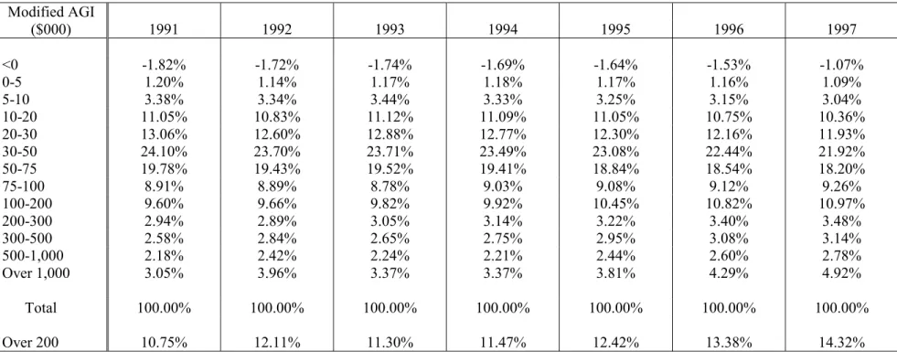
Table 2 gives a seven-year perspective on the recent surge in incomes at the top. In this table the income figures are based on a concept of modified adjusted income,
which excludes realized capital gains. It shows that the share of total income received by those returns with over $200,00 (1991 dollars) of income increased from 11.47% to 14.32%, or over one-fourth, between 1994 and 1997. Even more striking, the share received by those with income over $1 million increased from 3.37% to 4.92%, or nearly 50%! Some of this increase is certainly due to a larger number of returns in this category, but certainly not all.
The increase between 1994 and 1997 in the share of income received by high-income taxpayers is of at least the same order of magnitude as the increase between 1985 and 1988 which convinced nearly all observers, including Slemrod (1996), that, because this surge could not be explained by non-tax factors, the Tax Reform Act of 1986 must have been a major influence. It is less convincing to ascribe such a role for the Taxpayer Didn't Notice Act of 1995, or any tax change passed in 1994.
The sources of income growth between 1995 and 1996 are explored in greater detail in Table 3 (detailed data on 1997 is not yet publicly available). Here, taxpayers are ranked by Adjusted Gross Income (AGI), which includes capital gains. In just one year, the number of returns with incomes over $1 million increased by 27.5 percent, while AGI going to millionaires increased by 38.1 percent. Although in this case, capital gains was the fastest-growing source of income (71.2 percent) for this group, there was also
tremendous one-year growth in all other forms of income, such as a 29.9 percent increase in wages and salaries. By contrast, there was only a 1.6 percent increase in the total number of returns for people at all income levels, and a 5.1 percent increase in overall AGI.
Detail on higher slices of the income distribution is not yet available for the U.S. for these years, but some fascinating information from state income tax returns is
obtainable. Table 4 comes from 1995 and 1996 New Jersey income tax returns. While overall growth in New Jersey gross income was 7.6%, it was double-digit for all annual income classes over $250,000, and was nearly 50% for those families fortunate enough to have over $3 million in gross income! To be sure, much of the growth in the income of the highest class can be traced to the fact that the number of tax returns increased by over 40%, from 689 to 987, but the increase in the size of this group itself is a remarkable phenomenon.14
The source of the large gains at the top of the income distribution is also of interest. The total gross income increase of returns over $250,000 was $5.93 billion. Of that, almost none was in the form of interest and dividends. A total of 46.0% was employee compensation, 24.9% was capital gain, 9.5% was in partnership income, and 11.1% was in S corporation income.
7. Conclusions
"There's something happenin' here. What it is ain't exactly clear."
Stephen Stills
Our analysis of Section 6 suggests an extraordinary increase in the income, both realized and unrealized, of the already affluent beginning around 1996. What new light does this development shed on the chicken-and-egg ruminations of the first part of this essay?
First of all, it casts some doubt on the hypothesis that the top tax rate cuts of 1981 and 1986 were the key factor in generating the increases in measured inequality of the
last two decades. A decade passed between 1986 and 1996, with two top tax rate increase episodes in between, so it is difficult to link the recent surge in incomes at the top to tax policy. If the 1996 surge is not tax-related, it makes more plausible the case that the surge of 1986, of a similarly large magnitude, was not primarily tax-driven.
More importantly, the recent evidence suggests that the increase in inequality that began in the 1980's has not abated. If anything, the rate of increase dramatically
accelerated in the mid-1990s. Standard models suggest that the appropriate response to this development is an increase in the progressivity of the tax-and-transfer system. Models of public choice suggest that this may not happen.
In closing we note that during the preparation of this paper there were times in 1998 when we worried that our analysis of the stock market runup would seem
anachronistic, or even quaint, by the time of this conference. As of this writing (in early January, 1999), this worry has proven unfounded. But the uncertainty in the economic situation, and in particular the severe recessions in several Asian countries, remind us that the demand for progressivity as social insurance has not abated, and may be increasing.
Table 1
The Distribution of Income Under Alternative Definitions of Income
Mean income (in $thousands) Share of total income (%)
SCF, SCF, SCF, Treasury SCF, SCF, SCF,
Self- Income Income Family Self- Income Income
reported definition definition Economic reported definition definition
income (1) (2) Income income (1) (2)
Income rank Top 1 % 627.7 695.3 1013.8 14.3 14.3 14.2 17.8 95-99th% 159.7 196.6 242.5 13.9 14.6 16.0 17.0 90-94% 93.3 107.3 127.3 10.7 10.7 10.9 11.2 80-89% 68.2 75.5 83.4 16.0 15.6 15.4 14.7 Top quintile 120.8 138.7 172.7 54.9 55.2 56.5 60.7 60-79% 45.4 50.1 53.2 21.5 20.7 20.4 18.7 40-60% 29.6 31.4 32.7 13.3 13.5 12.8 11.5 20-39% 17.2 18.6 19.2 7.8 7.9 7.6 6.7 Bottom quintile 5.9 6.2 6.4 2.9 2.7 2.5 2.2 Overall 43.8 49.1 56.9 100 100 100 100
Source: 1995 Survey of Consumer Finances, unpublished distributional tables provided by the Treasury Department's Office of Tax Analysis for 1996, and authors' calculations.
Notes:
Households are re-sorted for each income definition.
Income definitions:
"Family economic income" is the income concept used by the Treasury Department in its distributional tables. It is based on the Haig-Simons definition of income, and imputes accrued capital income to tax return and Census data using a variety of data sources.
"Self-reported income" is the response to the SCF question on income, which counts income on a realization basis.
(1) Replaces reported capital income with a 6.4% real return to publicly-traded corporate equities, and a 3% real return to net worth other than business equity, but includes closely-held business income as reported.
(2) is the same as (1) but assumes a 28% real return to publicly-traded corporate
Table 2
Distribution of Modified Adjusted Gross Income, 1991-1997
Totals Modified AGI ($000) 1991 1992 1993 1994 1995 1996 1997 <0 -61,597 -60,698 -62,524 -63,942 -65,906 -65,446 -49,630 0-5 40,560 40,444 42,171 44.462 46,898 49,748 50,345 5-10 114,245 117,865 124,042 125,589 130,826 134,879 140,298 10-20 373,865 382,839 400,343 418,819 444,590 460,068 478,709 20-30 442,024 445,290 463,651 481,937 494,658 520,349 551,227 30-50 815,366 837,520 853,684 886,855 928,310 960,354 1,012,945 50-75 669,210 686,697 702,786 732,854 757,710 793,323 840,676 75-100 301,365 314,214 316,007 340,703 365,098 390,341 427,707 100-200 324,790 341,398 353,776 374,579 420,201 463,083 506,622 200-300 99,534 102,240 109.707 118,529 129,673 145,659 160,638 300-500 87,334 100,210 95,461 103,851 118,588 131,768 144,908 500-1,000 73,656 85,497 80,640 83,565 97,934 111,271 128,571 Over 1,000 103,138 139,973 121,234 127,086 153,162 183,772 227,327 Total 3,383,490 3,533,489 3,600,978 3,774,887 4,021,742 4,279,169 4,620,343 Over 200 363,662 427,920 407,042 433,031 499,357 572,470 661,444
Table 2 (continued) Shares Modified AGI ($000) 1991 1992 1993 1994 1995 1996 1997 <0 -1.82% -1.72% -1.74% -1.69% -1.64% -1.53% -1.07% 0-5 1.20% 1.14% 1.17% 1.18% 1.17% 1.16% 1.09% 5-10 3.38% 3.34% 3.44% 3.33% 3.25% 3.15% 3.04% 10-20 11.05% 10.83% 11.12% 11.09% 11.05% 10.75% 10.36% 20-30 13.06% 12.60% 12.88% 12.77% 12.30% 12.16% 11.93% 30-50 24.10% 23.70% 23.71% 23.49% 23.08% 22.44% 21.92% 50-75 19.78% 19.43% 19.52% 19.41% 18.84% 18.54% 18.20% 75-100 8.91% 8.89% 8.78% 9.03% 9.08% 9.12% 9.26% 100-200 9.60% 9.66% 9.82% 9.92% 10.45% 10.82% 10.97% 200-300 2.94% 2.89% 3.05% 3.14% 3.22% 3.40% 3.48% 300-500 2.58% 2.84% 2.65% 2.75% 2.95% 3.08% 3.14% 500-1,000 2.18% 2.42% 2.24% 2.21% 2.44% 2.60% 2.78% Over 1,000 3.05% 3.96% 3.37% 3.37% 3.81% 4.29% 4.92% Total 100.00% 100.00% 100.00% 100.00% 100.00% 100.00% 100.00% Over 200 10.75% 12.11% 11.30% 11.47% 12.42% 13.38% 14.32% Source: Office of Tax Analysis, U.S. Treasury Department. We are grateful to Bob Carroll for providing us with this information.
Notes:
Income classifier is Modified AGI in 1991 dollars. All totals are expressed in nominal dollars (in $millions).
Modified AGI defined as AGI minus capital gains in AGI and Social Security in AGI, plus tax-exempt interest income.
Table 3
Changes in Adjusted Gross Income and Income Sources, by Income Group, U.S., 1995-6 (in $ billions, except for number of returns column)
Size of Adjusted Gross Income
($000)
Tax Year No. of Returns Adjusted Gross Income Salaries and Wages Interest and Dividends
Capital Gains Partnership and S-Corp. Income Under $200 1995 116,954,819 3,549.30 2,896.05 213.29 64.79 24.53 1996 118,827,802 3,729.36 3,009.93 221.13 81.52 26.37 % Growth 1.6 5.1 3.9 3.7 25.8 7.5 $200 - 500 1995 1,007,136 292.12 174.56 31.75 24.93 32.18 1996 1,198,671 347.40 204.71 35.97 35.72 36.66 % Growth 19.0 18.9 17.3 13.3 43.3 13.9 $500 - 1,000 1995 178,374 120.35 60.21 15.99 15.99 20.34 1996 213,823 144.81 70.48 17.78 23.78 23.79 % Growth 19.9 20.3 17.1 11.2 48.7 17.0 More than $1,000 1995 86,998 227.58 70.64 36.86 64.71 48.70 1996 110,912 314.40 91.75 43.26 110.80 59.96 % Growth 27.5 38.1 29.9 17.4 71.2 23.1 Total 1995 118,218,327 4,189.35 3,201.46 297.89 170.42 125.75 1996 120,351,208 4,535.97 3,376.87 318.14 251.82 146.78 % Growth 1.8 8.3 5.5 6.8 47.8 16.7
Source: IRS Statistics of Income Bulletin, Fall 1998, and Individual Income Tax Returns 1995.
Interest and dividends includes both taxable interest, taxable dividends, and tax-exempt interest. Capital gains is defined here as taxable net gain less taxable net loss on Schedule D, plus capital gain distributions reported on Form 1040. Partnership and S-Corporation income is net income less net loss.
Table 4
Changes in Gross Income and Income Sources, by Income Group in New Jersey, 1995-6 (in $ billions, except for number of returns column)
Size of Gross Income
($000)
Tax Year No. of Returns Gross Income Employee Compen-sation Interest and Dividends
Capital Gains Partnership Income S-Corp. Income Under $250 1995 3,326,133 130.38 109.21 6.663 2.230 1.075 0.623 1996 3,337,510 136.36 113.37 6.812 2.895 1.103 0.765 % Growth 0.3 4.6 3.8 2.2 29.8 2.6 12.3 $250 - 500 1995 31,260 10.54 6.92 0.651 0.634 0.657 0.355 1996 36,085 12.17 7.91 0.703 0.894 0.716 0.434 % Growth 15.4 15.5 14.3 8.0 41.0 9.0 22.2 $500 - 1,000 1995 9,737 6.55 3.88 0.488 0.569 0.479 0.446 1996 11,083 7.45 4.37 0.497 0.780 0.556 0.486 % Growth 13.8 13.7 12.6 1.8 37.0 16.1 9.0 $1,000-3,000 1995 3,615 5.58 2.81 0.503 0.765 0.370 0.693 1996 4,394 6.74 3.32 0.514 1.087 0.485 0.827 % Growth 21.5 20.8 18.1 2.2 42.1 31.1 19.3 More than $3,000 1995 689 4.50 1.30 0.505 1.112 0.349 1.013 1996 987 6.74 2.04 0.504 1.794 0.660 1.348 % Growth 43.3 49.8 56.9 -0.2 61.3 89.1 33.1 Total 1995 3,371,434 157.55 124.12 8.81 5.31 2.93 3.13 1996 3,390,059 169.46 131.01 9.03 7.45 3.52 3.86 % Growth 0.6 7.6 5.6 2.5 40.3 20.1 23.3
Appendix Table A-1
Equity and Net Worth of Households, Ranked by Alternative Definitions of Income
Mean equities (in thousands) Net worth (in thousands) Equities as a share of net worth Self- Income Income Self- Income Income Self- Income Income reported definition definition reported definition definition reported definition definition
income (1) (2) income (1) (2) income (1) (2) Income rank Top 1 % 992.9 1273.0 1569.2 5078.2 5430.4 5581.9 0.196 0.234 0.281 95-99th % 204.3 214.2 230.3 1021.2 1146.6 1200.7 0.200 0.187 0.192 90-94% 85.0 91.0 79.3 452.5 504.4 573.3 0.188 0.180 0.138 80-89% 53.4 39.4 33.8 297.7 266.6 248.8 0.179 0.148 0.136 Top quintile 138.5 148.9 161.3 720.1 760.3 787.0 0.192 0.196 0.205 Next highest quintile 22.8 19.4 13.5 173.4 151.4 142.0 0.131 0.128 0.095 Middle quintile 9.8 8.2 4.3 105.9 104.0 95.2 0.093 0.079 0.045 Next lowest quintile 8.8 3.7 1.7 83.6 77.7 70.9 0.105 0.048 0.025 Bottom quintile 1.7 0.9 0.3 51.3 39.2 37.8 0.034 0.023 0.009 Overall 36.3 36.3 36.3 227.0 227.0 227.0 0.160 0.160 0.160
References
Alesina, Albert and Dani Rodrik (1994), "Distributive Politics and Economic Growth," Quarterly Journal of Economics, 109, 465-90.
Allen, Franklin (1982), "Optimal Linear Income Taxation with General Equilibrium Effects on Wages," Journal of Public Economics, 17, 135-43.
Atkinson, Anthony B. (1973), "How Progressive Should Income Tax Be?" in M. Parkin and A. R. Nobay (eds.), Essays in Modern Economics, (London: Longman), 90-109.
Auten, Gerald and Robert Carroll (1998), “The Effect of Income Taxes on Household Behavior,” The Review of Economics and Statistics, forthcoming.
Cameron, D. (1978), "The Expansion of the Public Economy: A Comparative Analysis," American Political Science Review, 72, 1243-61.
Carroll, Robert (1998a), “Do Taxpayers Really Respond to Changes in Tax Rates," mimeo, U.S. Department of the Treasury, Office of Tax Analysis Working Paper No. 78, August.
Carroll, Robert (1998b), “Tax Rates, Taxpayer Behavior, and the 1993 Tax Act,” paper presented at the 91st Annual Conference of the National Tax Association, Austin, TX, November.
Cilke, James, with Bob Gillette, C. Eric Larson, and Roy A. Wyscarver (1994), "The Treasury Individual Income Tax Simulation Model," mimeo, U.S. Department of the Treasury, Office of Tax Analysis.
Congressional Budget Office (1998a), The Economic and Budget Outlook: Fiscal Years 1999-2008, January.
Congressional Budget Office (1998b), The Economic and Budget Outlook for Fiscal Years 1999-2008: A Preliminary Update, July 15.
Congressional Budget Office (1998c), Estimates of Federal Tax Liabilities For Individuals and Families by Income Category and Family Type for 1995 and 1999. Memorandum, May.
Cooter, Robert and Elhanan Helpman (1974), "Optimal Income Taxation for Transfer Payments Under Different Social Welfare Criteria," Quarterly Journal of Economics, 88, 656-70.
Feenberg, Daniel and James M. Poterba (1993), “Income Inequality and the Incomes of Very High-Income Taxpayers: Evidence from Tax Returns,” in James Poterba (ed.), Tax Policy and the Economy, 7 (Cambridge, MA: MIT Press), 145-77.