A Performance Update Analysis

The Low-Income Housing

Tax Credit Program:

A Performance

Update Analysis

A CohnReznick LLP Report

This is the third in a series of periodic reports issued by CohnReznick LLP that address the performance of properties financed with federal low-income housing tax credits (housing tax credits) and funds organized to own interest in housing tax credit properties.

To compile and analyze the data required for the assessment, CohnReznick requested participation from every active housing tax credit syndicator and some of the nation’s largest institutional investors. Thirty-two of the 35 housing tax credit syndicators, and three of the nation’s largest investors, participated in the survey. For a complete list of study participants, please refer to Appendix A. CohnReznick analyzed data collected from 18,412 housing tax credit properties, focusing on how they performed during 2011 and 2012. For a more extensive discussion of the methodology employed to collect and analyze property data, please refer to Appendix B.

We are grateful to the housing credit industry for its continuing support of CohnReznick’s campaign to promote a deeper understanding of the housing tax credit program, its strengths, and the critical role it plays in the development of affordable housing.

COHNREZNICK LLP

November 2014

CohnReznick has used information gathered from the housing credit industry participants listed in Appendix A to compile this study. The information provided to us has not been independently tested or verified. As a result, we have relied exclusively on the study participants for the accuracy and completeness of their data. No study can be guaranteed to be 100% accurate, and errors can occur. CohnReznick does not guarantee the completeness or the accuracy of the data submitted by study participants and thus does not accept responsibility for your reliance on this report or any of the information contained herein. The information contained in this report includes estimations, approximations, and assumptions and is not intended to be legal, accounting, or tax advice. Please consult a lawyer, accountant, or tax advisor before relying on any information contained in this report. CohnReznick disclaims any liability associated with your reliance on any information contained herein.

To ensure compliance with the requirements imposed by the IRS, we inform you that any U.S. federal tax advice contained in this communication (including any attachments) is not intended or written to be used, and cannot be used, for the purpose of (i) avoiding penalties under the Internal Revenue Code or (ii) promoting, marketing, or recommending to another party any transaction or matter addressed herein.

Table of Contents

Chapter 1: Executive Summary

Chapter 2: The Convergence of Housing Tax Credits, Housing

Development, and the Banking Industry

Chapter 3: Regulatory Changes Impacting the State of the Equity

Market

Chapter 4: Fund Investment Performance

Chapter 5: Property Performance

Chapter 6: Portfolio Composition

Appendices:

Appendix A. Acknowledgements

Appendix B. Survey Methodology

Appendix C. Glossary

Appendix D. Property Performance – by State

Appendix E. Property Underperformance – by State

FIGURE 4.1 Portfolio Composition by Fund Type (Post 1999 Funds) by Gross Equity

FIGURE 4.1.1 Gross Equity Percentage of Multi-Investor and Proprietary Funds Since

1999

FIGURE 4.2.1 Gross Equity Price vs. Fund Yield by Year

FIGURE 4.2.2 Fund Yield vs. 10-Year Treasury Security Rate by Year

FIGURE 4.3.1 Fund Yield Variance by Year

FIGURE 4.3.2 Percentage Incidence of Negative Fund Yield Variance Since 1999

FIGURE 4.3.3 Median Fund Yield Variance by Year of Fund Closing

FIGURE 4.4.1 Housing Credit Delivery Variance by Investment Type

FIGURE 5.0.1 Overall Portfolio Composition

FIGURE 5.1.1 Overall Portfolio Performance

FIGURE 5.1.2 Overall Portfolio Performance (2008-2012)

FIGURE 5.1.3 Median Physical Occupancy

FIGURE 5.1.4 Median Debt Coverage Ratio

FIGURE 5.1.5 Median Per Unit Cash Flow

FIGURE 5.1.6 Median Net Equity Price by Year Placed in Service

FIGURE 5.1.7 Net Equity Price vs. Hard Debt Ratio-9% Credit

FIGURE 5.1.8 Net Equity Price vs. Hard Debt Ratio-4% Credit

FIGURE 5.2.1(A) Portfolio Distribution by Region

FIGURE 5.2.1(B) Operating Performance by Region

FIGURE 5.2.1(C) 2012 Median Physical Occupancy by Region

FIGURE 5.2.1(D) 2012 Median Debt Coverage Ratio by Region

FIGURE 5.2.1(E) 2012 Median Per Unit Cash flow by Region

FIGURE 5.2.2(A) 2012 Median Physical Occupancy by State

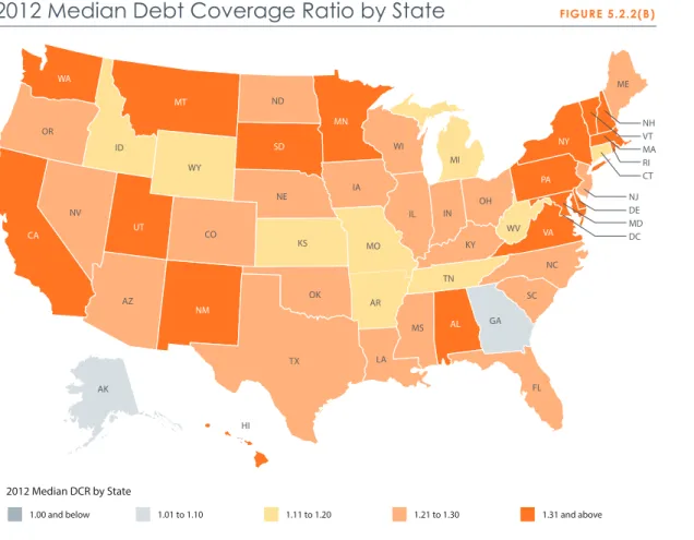
FIGURE 5.2.2(B) 2012 Median Debt Coverage Ratio by State

FIGURE 5.2.2(C) Median Debt Coverage Ratio by State (2008-2012)

FIGURE 5.2.2(D) 2012 Median Per Unit Cash Flow by State

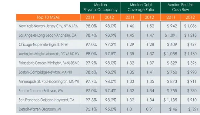
FIGURE 5.2.3 Operating Performance by Top 10 Metropolitan Statistical Areas

FIGURE 5.2.4(A) 2011 & 2012 Median Occupancy by Property Age

FIGURE 5.2.4(B) 2011 & 2012 Median DCR by Property Age

FIGURE 5.2.5 Operating Performance by Project Size

FIGURE 5.2.6 Operating Performance by Credit Type

FIGURE 5.2.7 Historical Hard Debt Ratio Trend

FIGURE 5.2.8 Operating Performance by Development Type

FIGURE 5.2.9 Operating Performance by Tenancy Type

FIGURE 5.3.1(A) Underperformance in 2011 & 2012

FIGURE 5.3.1(B) Underperformance in 2011 & 2012 by Unit Count

FIGURE 5.3.1(C) 2012 Per Unit Negative Cash Flow

FIGURE 5.3.2(A) Historical Underperformance Trend (2008-2012)

FIGURE 5.3.2(B) Historical Underperformance (2008-2012)

FIGURE 5.3.3 Chronic Underperformance

FIGURE 5.3.4(A) Distribution of 2012 Physical Occupancy

FIGURE 5.3.4(B) Distribution of 2012 Debt Coverage Ratio

FIGURE 5.3.4(C) Distribution of 2012 Per Unit Cash Flow

FIGURE 5.3.5(A) 2012 Occupancy Underperformance by State

FIGURE 5.3.5(B) 2012 Debt Coverage Ratio Underperformance by State

FIGURE 5.3.5(C) 2012 Per Unit Cash Flow Underperformance by State

FIGURE 5.3.6 Cumulative Foreclosure Rate by Year

FIGURE 5.3.7 Foreclosure County by Compliance Period Year

FIGURE 5.3.8 Reasons Indicated for Foreclosure 2008-2012

FIGURE 6.1 Percent Net Equity by Property Age

FIGURE 6.2 Unit Count by Year Placed in Service

FIGURE 6.3 Percent Net Equity by Investment Type

FIGURE 6.4 Percent Net Equity by Credit Type

FIGURE 6.5 Percent Net Equity by Development Type

FIGURE 6.6 Percent Net Equity by Tenancy Type

FIGURE 6.7 Portfolio Composition by Region

FIGURE 6.7(A) Percent Net Equity by Region

FIGURE 6.7(B) Average Project Size by Region

FIGURE 6.8 Percent Net Equity by State

W

e sometimes refer to the low-income housing tax credit as a housing

program hiding inside an Internal Revenue Code (IRC) section. IRC

Section 42, the housing tax credit statute, has now been a feature of the

IRC for 28 years, making it the longest-lasting federal housing program. No

one could have predicted at its enactment in 1986 that housing credits

would become the principal source of financing for the development

of affordable housing in this country. In fact, the housing credit program

has been responsible for the construction or rehabilitation of more than

2.5 million apartments.

Since its passage, an efficient capital market

for housing credit investments has evolved and, with it, sophisticated

information needs from the institutional investors that constitute that

market.

• In response to those needs, CohnReznick has undertaken a long-term effort to measure the economic performance of housing tax credit properties. By economic performance, we refer to how well housing credit properties are faring based on the traditional real estate metrics—occupancy, debt coverage ratio (DCR), and per unit cash flow. In addition, we assess whether investors are achieving the investment yields they have been promised and take an in-depth look at properties that are underperforming.

• The data demonstrate that the national portfolio of housing credit properties continues to perform well and that occupancy levels have remained remarkably strong over the years and across every type of project—large or small, urban, rural, or exurban, offering further

CHAPTER 1:

Executive Summary

evidence that there is a tremendous affordable housing shortage. The 2011 and 2012 nationwide median physical occupancy rate reached 97%, representing a high water mark for the industry. Normal turnover excluded, housing tax credit properties were nearly fully occupied, a result that should not be surprising given the national shortage of affordable housing.

• The median debt coverage ratio for housing tax credit properties hovered between 1.13 and 1.15 for a significant portion of the last decade before rising to 1.21 in 2009. Our analysis illustrates that the marked improvement in financial performance we witnessed during the recession years continued through 2012. The nationwide median DCR across housing tax credit properties we surveyed climbed to 1.30 in 2012.

• Perhaps the most striking development in the performance data has been the precipitous decline in the percentage of housing credit properties operating below breakeven. A property is operating at breakeven when its net operating income after funding replacement reserves is exactly equal to its debt service. The percentage of housing credit properties operating below breakeven, which reached a high point of 35% in 2005, fell by 43% to 20.2% in 2012.

• As strong as the performance metrics are, it is still the case that one in five properties operates below breakeven. That being said, only 10% of the surveyed properties incurred per unit deficits for the year 2012 in excess of $400. This explains why, in most cases, operating deficits are being funded through a combination of fee deferrals, operating reserves, and voluntary loans made by the general partners or syndicators.

• The cumulative rate of foreclosure in housing tax credit properties has risen somewhat over the years from 0.35% in 20052 _{to 0.57% in 2010 to 0.63% through the end of 2012.} While this might appear to suggest worsening performance, the bulk of the operating data clearly suggests that the opposite is the case. CohnReznick notes that foreclosure data may have been under-reported in previous years, in part because anecdotal evidence suggests that some of the defunct syndicators experienced a disproportionately higher incidence of foreclosures. Nonetheless, the incidence of foreclosures in housing tax credit properties continues to compare very favorably with the foreclosure rate of market rate multifamily properties and other real estate assets.

• While these data points are impressive, they do not provide an explanation for the nearly universal increase in property performance. As a result, we randomly surveyed 20% of the executives that run asset management departments for the survey respondents. Their commentary provides a more reliable basis for understanding improved performance than informed speculation on our part. Besides favorable debt leverage and more sophisticated underwriting that continued to positively influence property performance, contributing factors noted by the study participants included lower turnover and collection losses, and a general trend toward stabilization in rent and expense growth.

• “Our portfolio performance very closely mirrors CohnReznick’s data. We have seen occupancy tighten across our portfolio in terms of physical occupancy but, more important, in terms of economic occupancy. The rate of turnover in our properties has

steadily decreased over the past five years, which has meant fewer rent skips, better collections, and lower costs related to turning over and re-leasing our apartments.”

• “Property managers are reporting to us that rent collections have improved, which they attribute to employment gains and increasingly tight rental markets.”

• “Several years ago we were witnessing some real spikes in operating expenses, particularly in property insurance premiums, utility costs, and property taxes. More recently, our operating expenses have been more stable, although property taxes remain a problem in communities that are fiscally strapped.”

• “We own properties in some markets where rent increases have not been possible due to the lack of growth in area median income. For the most part, we have

been able to manage through the rent ceiling and are optimistic that improving

economic conditions will permit us to catch up in the future. In other markets, we have seen growth in rental income as tenants are no longer able to jump to competing properties—there simply are too few alternatives.”

• Whether the improvement in financial performance metrics can be sustained in the coming years will depend on a number of factors, including whether the industry continues to benefit from the historically low interest rate environment that it has enjoyed in recent years. Threats that could impact the program include 1) a version of tax reform that either removes the program or (more likely) “dilutes” its buying power, 2) local property taxation, 3) areas where median income has been flat or decreased, and 4) an increase in construction costs. CohnReznick is committed to conducting similar periodic studies to supply the industry with current and reliable data.

• While the use of technology has made advances, the housing credit industry is still a “horse and buggy” business compared to the quality of data that can be retrieved from the commercial real estate sector. Thus, for example, we received no data or incomplete data from survey participants when we asked them to report:

• Mortgage loan defaults

• Economic vs. physical occupancy

• Affordable Housing Investors Council risk ratings

Given the technology now widely available to sponsors and investors, we hope to retrieve and analyze these types of data as well as operating expense data when CohnReznick undertakes the next update.

T

he Low-Income Housing Tax Credit program reached the 28th

anniversary of its enactment in 2014. Adopted in the midst of dramatic

changes to the IRC in 1986 and made permanent in 1993, the program

has since enjoyed a strong level of bipartisan support in the United

States Congress. Moreover, it has become the most significant resource

for creating, rehabilitating, and preserving affordable housing in the

United States. While an exact unit count has not been compiled, the

U.S. Department of Housing and Urban Development estimates that

approximately 2.5 million affordable apartment units have been built

under the housing tax credit program since 1987. There are many factors

that have contributed to making the program successful, including

the fact that housing tax credit investments represent a public/private

partnership among the federal government, state housing agencies,

and the private sector.

Housing tax credits are allocated among the states by the federal government based on the states’ respective populations. Unlike most other tax expenditures, the cost of the housing tax credit program can be calculated with precision because the program’s funding authority is subject to a volume limit. The administration of the program resides primarily with the state credit allocating agencies, which have the authority to determine which projects should be awarded housing credits pursuant to a set of highly transparent procedures. As a result of its local control, the program has proven to be adaptable enough to serve changing housing needs as determined by the states annually. The real charm of the housing tax credit program, compared to every housing program which has preceded it, lies in the reliance on sophisticated capital.

CHAPTER 2:

The Convergence of Housing Tax Credits,

2.1 How is a Typical Housing Tax Credit Project Financed?

The process begins with a developer gaining control of a developable parcel and initiating the process of securing building permits, environmental clearance, access to utilities, and support of local officials. This can be a multiyear effort in many parts of the country. Once the developer has site control, it can apply for an allocation of housing credits from the relevant state agency. The application process is fraught with its own set of perils because there simply are not enough housing credits available to meet the demand. The states publish their procedures for making allocation decisions annually in a document known as a qualified allocation plan. It is not uncommon for states to turn away three to four applicants for every project that receives a reservation of credits.

Once a developer has a credit reservation in hand, it can negotiate with equity investors, syndication companies, and construction lenders and search for supplemental sources of capital from state and local governments. For most of the past 15 years, the demand for housing credit investments has exceeded the supply. The demand for credits has driven the price at which they trade from $0.42 per $1.00 of housing tax credits in the early years of the program to close to $1.00 per $1.00 of housing tax credits as of the date of publication of this report. The steady progression in housing credit prices has changed the “capital stack” in financing these developments. It is not uncommon for housing credit projects to be financed 75-80% with investor equity, with the balance coming from conventional mortgage financing and, in some cases, “soft” financing from governmental lenders.

This unique combination of capital sources allows housing credit properties to be financed with low levels of “must pay” debt. Ultimately, it is the sparing use of leverage that allows developers to be able to rent these apartments to tenants who could otherwise never hope to live in safe, decent, affordable housing. It is for this reason that the housing credit program is referred to as a capital subsidy.

2.2 How Does the Public/Private Partnership Foster an Efficient

Use of the Capital Subsidy?

Compared to rental subsidy programs, the housing tax credit model has proven to be much more efficient.

• State allocating agencies are statutorily obligated to award only enough housing tax credits to make potential developments financially feasible, and the agencies have become very effective at ensuring that the projects to which they award housing credits are not overfinanced.

• In addition to the underwriting that housing credit projects undergo at the state agency level, these developments are underwritten by lenders, investors, and syndicators who acquire, underwrite, and asset manage these investments for institutional investors. These players typically have sophisticated real estate underwriting platforms that initially supported conventional multifamily or other types of real estate assets. By leveraging their existing underwriting platforms, recruiting talented real estate professionals, and using similarly rigorous underwriting criteria (while acknowledging the uniqueness of this

• Before enactment of the housing tax credit program, there were drastic differences in the management of conventional multifamily real estate and affordable housing. Much of the pre-housing credit affordable housing inventory was composed of public housing built in the 1950s and 1960s and rental housing built in the 1960s and 1970s that was financed with a variety of Department of Housing and Urban Development (HUD) subsidies. The “older assisted inventory,” as it is sometimes referred to, has not stood the test of time because of design flaws, inadequate maintenance, and, in some cases, poor management. In contrast, housing credit projects tend to look, feel, and operate as if they were conventional multifamily apartments. These properties, as a class, have been more professionally managed by private sector operators and managers.

• In addition to generating tax equity, housing tax credit investments attract private capital from debt providers that would otherwise be disinclined to lend to affordable housing projects. While the debt coverage, typically 1.15-1.20, affords a fairly modest buffer to break even, the lenders that operate in this space understand that the quality of the cash flows in these projects, fueled largely by the demand for the units, is actually quite high.

• Ultimately, the success of housing tax credit investments is collectively “guaranteed” by stakeholders that share common goals. Over time, numerous mechanisms have been built into the development and management processes to hold different participants accountable for their performance, such as payment and performance bonds for general contractors, development completion guarantees for developers, operating deficit guarantees and various tax credit guarantees, and compliance and long-term use restriction requirements for all parties.

2.3. Why Do Institutional Investors Invest in Housing Tax Credit

Investments?

Since the mid-1990s, the equity market for housing tax credit investments has been predominantly composed of large, publicly traded companies, most of which are in the banking and financial services sector. As investors and regulators have become increasingly confident in the financial performance of housing tax credit properties as an asset class, the housing tax credit program has become more dependent on the banking sector as a highly reliable source of equity to meet its capital needs. This has been a largely favorable development because banks, for example, filled most of the equity gap created when Fannie Mae and Freddie Mac exited the housing credit market in 2007 and 2008. CohnReznick estimates that approximately $11 billion of capital was committed to housing tax credit investments in 2013, and that the banking sector was the source for approximately 85% of that amount. There are a number of factors that make housing tax credit investments attractive to banks:

• Increasing after-tax earnings and lowering effective tax rate: Housing credit investors are effectively purchasing a financial asset in the form of a stream of tax benefits (consisting of tax credits and passive losses associated with depreciation and mortgage interest deductions). Investors do not anticipate receiving cash flow distributions, because housing tax credit properties are generally underwritten to slightly above breakeven and developers or syndicators are generally the recipients of any remaining cash flow. Substantially all of the investors’ returns are expected to be derived from tax benefits. Banks typically report fairly stable earnings from year to year and are thus predictable federal taxpayers having sufficient taxable income against which to offset tax credits. The housing tax credit is earned over a 15-year period but is claimed over an accelerated 10-year timeframe, beginning in the year in which the property is placed in service and units are occupied. The ideal housing credit investor is a company with a track record of consistent growth in earnings that is a regular rather than an alternative minimum taxpayer. This has been the profile of the U.S. banking industry for most of the last 28 years, with the exception of rare recession-driven interruptions.

• Satisfying CRA lending and investment test objectives: Banks are obligated, under the Community Reinvestment Act (CRA) regulations, to make loans, provide services, and make investments in low- to moderate-income neighborhoods in those areas in which they conduct business. As a regulatory matter, banks are obligated to operate in a “safe and sound” manner, which requires them to avoid investments that represent potential loss of capital. The strong financial performance track record of housing tax credit investments has historically been an ideal match for bank investors with a conservative focus. There are a limited number of qualified equity investments under CRA regulations, and many of these have less attractive yield and/or risk profiles. Among the available investment options, housing credit investments appear to be a clear investor favorite.

• Achieving a reasonable/superior risk adjusted rate of return: The banks that CohnReznick surveyed have advised us that on a risk-adjusted basis, the yields generated by their housing credit investments are superior to most of their available community development investment alternatives. This is, in part, because banks enjoy a lower cost of funds than other investors, which widens the spread between that cost and the rate of return offered by housing credit investments.

• Enhancing community relations and searching for cross-selling opportunities:

Notwithstanding their CRA objectives, U.S. banks have become sophisticated housing tax credit investors and have learned to leverage their equity investments to sell other products and services to the development community. Thus, we increasingly see banks cross-selling other services such as construction financing, letters of credit, permanent loans, and other products to the properties in which they invest.

C

orporate investors typically determine their annual tax credit investment

volume based largely on their projected taxable income. Since

the global recession, the earnings profile of most financial services firms

has become more reliable. Stable earnings in this sector coupled with

access to low-cost capital has fueled renewed appetite for tax credit

investments. Further, because the supply of housing tax credits is largely

fixed by statute and comprehensive tax reform has not been undertaken

since 1986, it has been relatively straightforward for a financial institution to

forecast tax liabilities and benefits over the 10-year credit delivery period.

As noted, CohnReznick estimates that in 2013 the housing tax credit market saw nearly $11 billion of new investment, 85% of which we believe is attributable to capital provided by the banking sector. The steady flow of capital invested by the national banks has made it possible for the low-income housing tax credit to mature and thrive. While the industry learned that it was over-reliant on the banking sector in 2008 and 2009, it has also become clear that stable tax and regulatory environments ensure the reliable presence of bank investors. The bottom line is that capital from community reinvestment act motivated banks is now the lifeblood of the housing credit program.

Although the tax credit market is thriving, a number of recent regulatory initiatives may affect the future of the equity market for housing tax credits. In 2013, there were policy changes in three areas that may directly impact bank participation in the housing credit market: new regulations under the CRA, Basel III, and new financial reporting rules from the Financial Accounting Standards Board (FASB). The following narrative provides an update on each topic and explores the potential impacts on investor demand going forward.

CHAPTER 3:

Regulatory Changes Impacting

the State of the Equity Market

3.1. Implication of New CRA Regulation

In November 2013, financial institutions received much anticipated clarification from the Office of the Comptroller of the Currency, the Board of Governors of the Federal Reserve System, and the Federal Deposit Insurance Corporation (the Agencies) in their revised Interagency Questions and Answers Regarding Community Reinvestment (Questions and Answers). The Agencies, among other things, affirmed that community development loans and qualified investments located outside of a bank’s assessment area(s) can receive positive consideration toward meeting the CRA objectives, provided that the “institution is being responsive to the community development needs and opportunities in its assessment area(s).”

While an institution’s performance within its assessment area(s) remains the primary focus of CRA examination, this change in the regulations may begin to address the imbalance in housing credit pricing seen between metropolitan (CRA hot) and non-metropolitan (CRA not) markets. The sometimes stark difference in the “CRA value” of housing credit projects depending on their location was analyzed and documented in a May 2013 CohnReznick study, The Community Reinvestment Act and Its Effect on Housing Tax Credit Pricing. Differential tax credit pricing results in fewer investment dollars going to affordable housing developments located in CRA not areas and means that some projects, particularly in rural areas, cannot be financed.

Since the new regulations were issued, the agencies have amended their examination procedures to allow institutions to more clearly identify LIHTC investments located in statewide or regional areas that include but may not directly impact their assessment areas.

Implementation of the revisions is already underway, with the Agencies having provided standardized forms and training for CRA examiners. Many banks are waiting to see how their field examiners interpret the revised regulations when giving “credit” for investments in projects acquired by nationwide and regional funds that fall outside their self-defined assessment areas. The largest national banks, which have the most at risk in terms of securing high ratings, have advised CohnReznick that while the Questions and Answers are helpful, they will wait to see CRA exam results before they can be comfortable and confident with how the new rules are being implemented.

3.2 Banking Regulatory Environment

In response to the 2008-2012 global banking crisis, representatives from international banking authorities set forth proposed regulations to address systemic risk resulting from the interconnectedness of the world’s financial system. Under what is commonly referred to as the Basel III capital framework, financial institutions are subject to increasingly stringent minimum capital requirements, limitations on their ability to recognize deferred tax assets in their financial statements, and tougher risk weighting of real estate assets, among other restrictions. The Office of the Comptroller of the Currency and the Board of Governors of the Federal Reserve System published a final rule on October 11, 2013, that established a new regulatory capital framework, which incorporates aspects of Basel III and replaces existing risk-based and leverage capital rules.

When developing the new capital regulations, the Agencies recognized the unique nature of community development finance vehicles, such as housing credit investments. The agencies decided that certain of the new regulatory requirements should not apply to equity investments in and mortgage loans to affordable housing projects. For instance, Basel III proposed to apply a 150% risk weighting to so-called High Volatility Commercial Real Estate exposures (HVCRE) with high loan to value, a regulatory change that could have negatively affected financing for housing credit projects. Based in part on advocacy from the housing credit industry and the low foreclosure rates in this asset class, the definition of HVCRE was amended explicitly to exclude loans that finance community development investments.

The final rule also provided preferential capital treatment to equity investments made under the public welfare authority, including housing credit investments. Unlike other equity exposures that could receive risk weights as high as 400%, housing credit investments will be subject to a 100% risk weight.

The risk weighting of a bank’s assets is significant because the final rule increases the minimum capital ratios that financial institutions must satisfy in order to be considered adequately capitalized. The key regulatory measure of capitalization (Tier 1 ratio) compares Tier 1 capital to risk-weighted assets.

Under the existing regulatory capital rule, in order to be adequately capitalized, a bank was required to have a minimum Tier 1 ratio of 4% and a 6% ratio to be considered well capitalized. Basel III requires a 4.5% minimum capital ratio for the common equity component of Tier 1 capital.

As a result, financial institutions will be required to reserve a greater percentage of their capital assets. The reduction of available capital could impact the amount of capital available for tax credit investments once it goes into effect after January 1, 2015. Since financial institutions will be required to hold a greater percentage of their assets in liquid, low-yield accounts, banks will need to generate more favorable returns on the capital that is invested. The need for higher returns could drive down tax credit pricing and increase the cost of capital for housing credit projects.

3.3 Implications of the New Accounting Change

In 1994, the Emerging Issues Task Force (EITF) of the FASB considered for the first time how LIHTC investments should be accounted for. As a result of their deliberations, in May of 1995, the Task Force issued EITF 94-1, now referred to as ASC 970, which sets out the general principles for accounting for housing tax credit investments. That guidance provided that LIHTC investments that were not coupled with a yield guarantee must be accounted for under either the cost or equity method of accounting. Under the equity method, an investor’s net income from operations is artificially depressed by depreciation-driven equity losses and impairment adjustments related to project investments. The benefit of housing credits, however, is not reflected in pre-tax income and instead is reflected in the income tax provision.

Basel III Minimum Capital Requirements

2012

2015

Risk Weighted Assets

500

500

Capital Requirements

x4%

x6%

Reporting the results of housing credit investments in different sections of the financial statement has made it difficult for the reader of a company’s financial statements to understand the real investment impacts of housing credit investments.

In the fall of 2010, the FASB was persuaded to take up once again the issue of accounting for housing tax credit investments. Consensus was reached in late 2013 and culminated in the issuance of Accounting Standards Update (ASU 2014-01) on January 15, 2014. Most significantly, the ASU 2014-01 established a new accounting method, referred to as the “proportional amortization method,” which represents a significant departure from the equity method. Under the new method, amortization of the investment is reflected as a component of the investor’s income tax expense rather than as a reduction of operating income on its income statement. Under the proportional amortization method, housing credit investments are presented on a “net, net basis” whereby the amortization, tax credits, and other tax benefits are all reflected in the income tax expense line. While the accounting method change will not change bottom-line earnings, the book losses from LIHTC investments will no longer represent a drag on pre-tax net operating income for investors that elect the new method. In addition, bank investors will be able to report lower non-interest expense, an income statement line item, which factors into how their operating efficiency is measured.

.

ASU 2014-01 has generated much attention and interest from housing credit investors. Housing credit investors are now obligated to disclose the amount of housing credits and related tax benefits they claim each year, the impact on their income tax expense, and the carrying value of their LIHTC investments (without regard to the accounting method they chose). Implementing the proportional amortization method has proven challenging for most investors with large portfolios. Nonetheless, we believe it will be the preferred method going forward because of its lower administrative burden and the improved income statement presentation compared to the equity method.

Equity Method

Proportional Amortization

• Equity loss no longer used • Impairment is only relevant when it occurs when tax credits and other tax benefits no longer expected to be received

The ability to use proportional amortization may result in fewer so-called “guaranteed yield” transactions, because the primary motivation for companies that chose to make guaranteed yield investments was to avoid having to use equity accounting. However, since the economic fundamentals of housing credit investing have not changed, we expect that any growth in the investor base will likely be at the margins rather than a fundamental market shift.

CHAPTER 4:

Fund Investment Performance

G

enerally, an investor contemplating investing in housing tax credits

can choose from one of two investment approaches:

a direct

investment

or

a syndicated investment

. Under the direct investment

model, an investor directly owns a limited partner interest in the property

partnership that owns the underlying property, with the developer typically

assuming the general partner interest. The direct investment approach is

typically feasible only for investors that have internal resources dedicated

to the acquisition, underwriting, and asset management of housing

tax credit properties. As a result, this approach is favored by a handful

of institutional investors. The syndicated investment approach enables

investors to invest in a fund organized and managed by third-party

intermediaries known as syndicators. The investor(s) own the limited

partner interest in the fund, with the fund in turn owning the limited partner

interest in various property partnerships.

There are two primary investment options when working with a syndicator: proprietary funds and multi-investor funds. In both cases, the syndicator originates potential property investments, performs underwriting, and presents the potential investment to investors. Proprietary funds are typically sought out by a single investor with a desire for a higher level of control over the location of the properties they finance. The CRA requires banks to make qualified investments in areas in which they collect deposits, and they consequently receive CRA “credit” for doing so. Therefore, one of the primary investment motivations for banks is to earn CRA credit through their housing credit investments. Proprietary funds are a common investment option for institutions that want to focus their capital into very specific locations. The principal advantage of a multi-investor fund is risk diversification. A multi-investor fund can be composed of a number of investors, all of whom share risk and rewards based upon their proportional equity contribution to the fund.

Whether the fund has one or many investors, certain tax credit funds are credit-enhanced either by the syndicator or, more typically, by a third-party insurance company. Traditionally, approximately 20% of all tax credit investments were structured with a minimum yield guarantee. In previous years, an advantage of a credit-enhanced housing credit investment, other than its guaranteed minimum return, was the ability to use the so-called effective yield accounting method. However, the disadvantage of a guaranteed fund is that a substantial portion of the investor’s capital is used to finance the guarantee fee, resulting in a substantially lower investment yield. More recently, yield guarantees have become rarer, because of the lack of creditworthy guarantors. In addition, as previously noted in Chapter 3 of this report, the ability of investors to use the proportional amortization method of accounting has stripped guaranteed investments of one of their most beneficial advantages over conventional housing credit investments. CohnReznick suspects that, because of the reasons noted above, guaranteed investments may become less and less common. Regardless of the chosen investment vehicle, low-income housing tax credit investors are effectively purchasing a financial asset in the form of a stream of tax benefits. Investors do not anticipate receiving cash flow distributions, because housing tax credit properties are generally underwritten to operate just above breakeven and developers or syndicators are generally the recipients of any excess cash flow.

4.1 Investment Performance

Survey respondents were asked to supply CohnReznick with performance data for every low-income housing tax credit fund that they syndicated. Our analysis of fund-level performance data assesses the track record of housing credit funds’ delivery of the originally projected yield and credits to investors versus their actual results.

The yield from housing credit investments is generally measured by the investment’s after-tax internal rate of return (IRR). The IRR is a function of the amount and timing of the projected housing credits and profit/loss versus the timing of the investor’s equity pay-in. In general, housing tax credits are realized on a straight-line basis over a 10-year period. Tax credits not delivered to investors in the first year because of construction or lease-up delays are typically realized in the 11th year (unless there is a permanent tax credit shortfall, which is often covered by basis adjustors). Most housing credit investments are structured with one or more “true-up” provisions to assist with yield maintenance. For instance, a loss of the time value of credits can be compensated for by a so-called adjustor provision that reduces the investor’s remaining capital contributions to maintain the projected yield. It is important to note that, in addition to the timing of tax credit realization, the composition of the tax benefits (the relative proportion of tax credits to tax losses) is equally important to investors. Traditionally, investors who are sensitive to the negative impact of losses on their earnings were more inclined to invest in 9% tax credit properties with low leverage and less inclined to invest in 4% credit tax-exempt bond transactions that are more highly leveraged. However, given the fact that 4% properties perform roughly the same as 9% properties and in light of the introduction of the proportional amortization method of accounting, the investor bias against 4% properties is likely

Twenty-three survey respondents provided data for 1,140 low-income housing tax credit funds. For purposes of this analysis, we removed all funds that were closed in 1998 or earlier, as the property investments of these funds had already surpassed their 15-year compliance periods as of the effective date of this report. Figure 4.1 illustrates the remaining 893 funds that closed in or later than 1999, organized by fund type and segmented by gross equity and low-income housing tax credits. The average age of the 893 funds presented was eight years as of the effective date of this report.

Of the 893 funds, there were 368 multi-investor funds accounting for 53.3% of the surveyed gross equity with an average fund size of $77.5 million of gross equity. The 486 proprietary funds in the pool accounted for 44.7% of the total fund portfolio gross equity, with an average fund size of $49.7 million of gross equity. The difference in the average size of these funds is driven by the fact that multi-investor funds are typically larger to accommodate the investment objectives of multiple investors. The remaining 39 funds were either guaranteed yield investments or public funds sold to individual investors. These fund types accounted for a total of 2.0% of the total gross equity.

Proprietary

Multi-Investor

Guaranteed

Public

1.7% 0.3%

53.3%

44.7%

Figure 4.1

Portfolio Composition by Fund Type

Figure 4.1.1 illustrates the historical gross equity percentage split between multi-investor and proprietary fund investments since 1999. Not surprisingly, the percentage of proprietary funds reached its high point at 72.1% in 2009, when the housing credit market was at its lowest point. At the height of the recession, housing credit investors that remained active were almost entirely focused on meeting their CRA obligations, and deployed their capital predominantly through proprietary funds. After the equity market rebounded from the recession, the syndication of multi-investor funds also rebounded, reaching 64.5% in 2012.

4.2 Fund Yields

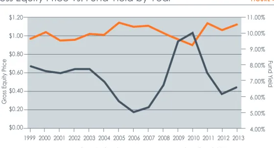
Figure 4.2.1 illustrates the historical relationship between gross equity price and fund investment yields. Dramatic financial and organizational changes within what had been the market’s two largest housing credit investors, Fannie Mae and Freddie Mac, occasioned their exit from the housing credit equity market in 2007 and 2008. In addition to the loss of these government-sponsored enterprises (GSEs) as investors, the devaluation of mortgage securities and subsequent collapse of financial markets severely decreased the demand for tax credit investment among the nation’s largest financial institutions. The cumulative effect of losing the GSEs as investors and losses in the banking sector resulted in a 50% cumulative drop in tax credit demand from the market highs observed in 2006.

Multi-Investor Fund % Proprietary Fund %

1999 2000 2001 2002 2003 2004 2005 2006 2007 2008 2009 2010 2011 2012 100% 90% 80% 70% 50% 40% 30% 20% 10% 0% Figure 4.1.1

Gross Equity Percentage of Multi-Investor

Figure 4.2.1 also demonstrates relatively steady tax credit pricing of between $0.95 and $1.10 per $1.00 of credit despite the relatively drastic fluctuation of yields. During the down years of the national recession when yields exceeded 10%, the median gross equity price dipped to its lowest point, $0.90. While that median will strike some as very high given market conditions, it should be noted that tax credit pricing remained stubbornly high in the “hottest” CRA markets. When the equity market rebounded to pre-recession levels, yields decreased in kind while pricing returned to the high end of the pricing range exhibited in previous years.

Figure 4.2.2 illustrates the historical relationship between housing tax credit fund yields and 10-year Treasury security yields (adjusted for an after-tax rate equivalent of a 35% tax rate). The chart depicts the median originally projected housing tax credit yield by year and the annual trend in 10-year Treasury security yields. In 2006 and 2007, housing credit fund yields approached Treasury yields, but have since increased and were subsequently diverted significantly in the next three years. The rates have since converged to some degree, but housing credit fund yields continue to represent a significant premium over the yield from long-term Treasury securities.

$1.20 $1.00 $0.80 $0.60 $0.40 $0.20 $0.00 11.00% 10.00% 9.00% 8.00% 7.00% 6.00% 5.00% 4.00% 1999 2000 2001 2002 2003 2004 2005 2006 2007 2008 2009 2010 2011 2012

Gross Equity Price

Gross Equity Price

Annual Median Yield

Fund Yield

2013

Figure 4.2.1

4.3 Yield Variance Analysis

It is important to consider the performance of housing tax credit funds with respect to actual income tax benefits versus originally projected benefits. Investment performance is expressed in terms of yield (calculated based on a quarterly after-tax internal rate of return), overall tax credit delivery, and the initial years of tax credit delivery relative to originally projected amounts.

As we have defined the term, yield variance measures the difference between the originally projected yield at investment closing and the most current yield projection (December 31, 2012, for purposes of our survey). Positive variances indicate the achievement of greater than projected yield. On a weighted average basis (where yield variances for individual funds are aggregated and weighted by equity), survey respondents reported a positive 6.45% variance in meeting yield targets. We removed housing credit funds with credit enhancement (“guaranteed funds”) from this analysis because guaranteed funds are structured with yield maintenance mechanisms that ensure a predictable yield to investors. While yield is a significant factor for housing credit investors, the individual components of yield computations have a major bearing on their calculation. Yield can be maintained naturally or artificially by pre-negotiated investment provisions in a number of ways. An investor can receive a more favorable yield in a number of ways: as a result of an underperforming portfolio generating higher losses, if equity pay-in schedules are adjusted to postpone capital contributions, or if so-called adjustor provisions, under which remaining investor capital contributions are reduced to the extent necessary in order to re-establish the target yield.

12.00% 10.00% 8.00% 6.00% 4.00% 2.00% 0.00% 1999 2000 2001 2002 2003 2004 2005 2006 2007 2008 2009 2010 2011 2012

Annual Median Yield of Housing Credit Funds 10-Year Treasury Yield (after tax equivalent)

2013

Fund Yield

Figure 4.2.2

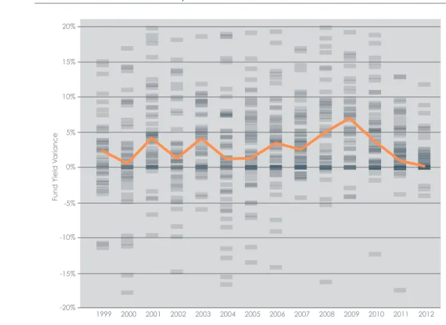
Figure 4.3.1 illustrates the variation in fund yield performance based on the year in which the funds were closed.

The graph illustrates the fact that 16.1% of the funds CohnReznick studied reported negative yield variances.3 _{We totaled the negative yield variances relative to the overall number} of funds closed in each year and found that the years during which funds with the highest incidence of negative variance were syndicated in 1999, 2000, 2002, 2004, and 2005. Not coincidentally, those same years have among the highest number of funds syndicated relative to all other years surveyed. Based purely on the percentage of funds with negative yield variances relative to the total number of funds syndicated in the same year, it appears that more recently syndicated funds are generating more favorable results. Indeed, funds closed in years later than 2006 reported fewer than a 12% incidence of negative yield variances. Figure 4.3.2 illustrates the percentage of funds with negative yield variances sorted by the year in which they initially closed.

2012 2011 2010 2009 2008 2007 2006 2005 2004 2003 2002 2001 2000 1999 0% 20% -20% -10% -15% -5% 5% 15% 10% Fund Y ield V ariance

Figure 4.3.1 – Fund Yield Variance by Year

The data illustrate that “younger” funds with early-stage properties generally perform better. As such, the most recent years in the table above illustrate very low instances of negative yield variance. Note that any year when fewer than 30 surveyed funds were reported to have closed was removed from our analysis.

Figure 4.3.3 illustrates the median fund yield variance by year closed since 1999.

As the table above indicates, aside from a few outlier years since 1999, proprietary funds have reported larger median yield variance than their multi-investor counterparts. We note, however, that the magnitude of the variance between the two fund types could be affected by the manner in which syndicators define “original” yields, especially for proprietary funds that tend to be less specified at closing. We hesitate to draw too many conclusions from this comparison, given the variability between syndicators’ internal processes for tracking proprietary yield data.

1999 2000 2001 2002 2003 2004 2005 2006 2007 2008 2009 2010 2011 2012 8.0% 7.0% 6.0% 5.0% 4.0% 3.0% 2.0% 1.0% 0.0%

Fund Yield Variance

Median Proprietary Fund Variance Median Multi-Investor Fund Variance

Median Fund Yield Variance by Year of Fund Closing

Percentage Incidence of Negative Fund Yield

Variance Since 1999

30.6% 33.9% 9.7% 31.3% 17.3% 31.7% 21.9% 16.1% 11.1% 10.2% 5.6% 5.8% 6.7% 5.9%

Percent incidence of negative yield variance

4.4. Housing Credit Variance Analysis

Consistent with CohnReznick’s industry experience, the survey data we examined demonstrated that the aggregate average variance in total housing credits has been less than 1%. Investors were projected to receive $53.0 billion in credits and actually received $52.6 billion through 2012.

The average housing credit investment derives the majority of its benefits (roughly 75%) from housing credits, with the balance coming from passive losses. Because housing tax credits are calculated based on qualified development costs, a property’s future delivery of tax credits is highly predictable. In this context, the timing of tax credit delivery is more likely to create variances, because delays in the construction and lease-up of housing credit properties may result in delayed delivery of housing credits. Our data suggest that such delays, not uncommon in the early years of the program, have become less common over time as the industry’s ability to underwrite credit delivery has improved.

While the total housing credit delivery variance increased slightly since our last study from a (-0.4%) to (-0.8%), the industry continues to show improvement in projecting first year credits. There is a significant gap between proprietary and multi-investor funds’ first- and second-year variance of housing credit delivery. While this gap has decreased since our last performance study, the relationship remains between the two fund types. We presume the difference to be attributable to the fact that proprietary funds are, on average, less specified than their multi-investor counterparts. Because proprietary funds tend to be less specified, comparing actual credit delivery results to original projections may not be as objective an analysis as multi-investor funds, and thus we focus on the track record of multi-investor funds.

Housing Credit Delivery Variance by Investment Type

Total -0.8% -7.1% -10.1% -6.5% Proprietary -1.3% -3.0% -6.9% -5.0% Multi-investor -0.5% -10.8% -13.1% -7.9% Guaranteed 1.0% -4.5% -2.1% 1.4% Total Housing Credit Delivery Variance 1st-Year Housing Credit Delivery Variance 2nd-Year Housing Credit Delivery Variance 3rd-Year Housing Credit Delivery Variance

C

ohnReznick solicited data from 35 active housing tax credit syndicators

and a number of the nation’s largest housing credit investors,

hereinafter referred to as “data providers” or “respondents.” Thirty-two

syndicators participated and provided portfolio data, which equates to

approximately a 91% response rate. Those who did not participate were

predominantly smaller organizations for which the administrative burden

of providing data within our desired timeframe as deemed too onerous,

or those who were newly formed organizations that manage just a handful

of stabilized properties. In addition to the syndicator respondents, three

of the largest housing credit investors provided data. In an effort to avoid

reconciling property investments held in shared portfolios, we collected

only direct investment data from investor respondents. All data were to

investors provided by the respondents to CohnReznick on a voluntary and

strictly confidential basis.

This chapter summarizes the operating and financial data collected from the respondents for housing tax credit property investments located in each of the 50 states, the District of Columbia, Guam, the U.S. Virgin Islands, and Puerto Rico. The data gathered represented 18,412 housing tax credit properties, an increase of more than 1,000 properties from our most recent study, which analyzed 2008-2010 operating performance. All participants in this study also participated in our 2010 study. The increase in sample size reflected the net increase as additional properties were placed in service and older properties at the end of their respective compliance periods were disposed of. We estimate that this data sample represents approximately 70% of the entire inventory of housing tax credit properties that are actively managed by syndicators and/or investors. The gap between CohnReznick’s data sample and the entire housing tax credit inventory can be attributed to investments made by syndication firms that have left the business, and properties that have reached the expiration of their respective compliance periods and subsequently “cycled out” of the program.

CHAPTER 5:

Property Performance

As can be observed in Figure 5.0.1, the 18,412 properties in CohnReznick’s data sample collectively represented approximately $76 billion in net equity investments and approximately $80 billion in housing tax credits. CohnReznick notes that some respondents did not provide either/or equity and housing credit information for some of the properties in their portfolio. As such, the net equity and housing credit totals are understated.

Of the 18,412 properties, 15,588 (84.7%) achieved “stabilized operations” as of December 31, 2012. We characterize a property as having achieved “stabilized operations” when it has completed construction, achieved 100% tax credit occupancy (when all of the tax credit units have been occupied by income-eligible tenants), and has closed on its permanent financing. While the definition of stabilized operations differs slightly among industry participants, CohnReznick has adopted the industry’s consensus definition and does not believe these slight differences are material enough to distort the analysis.

5.1 Portfolio Performance Data—Physical Occupancy, DCR

and Per Unit Cash Flow

CohnReznick measured the real estate performance of the surveyed properties by using a number of operating and financial metrics, including:

• Physical occupancy, defined as the number of units occupied divided by the number of units available. While we would prefer to report both physical and economic occupancy rates, only a small subset of surveyed syndication firms track economic occupancy data for their portfolios.

• Debt coverage ratio, defined as net operating income less required replacement reserve deposits, divided by mandatory debt service payments.

• Per unit cash flow, defined as the total cash flow generated after deducting debt service

payments and required replacement reserve contributions, divided by the total number of units within the property.

Overall Portfolio Composition

Number of Properties 18,412 15,588 84.7%

Number of Units 1,369,239 1,193,244 87.1%

Number of LIHTC Units 1,317,984 1,138,418 86.4%

Housing Credit Net Equity $ 76,117,190,987 $ 61,737,621,507 81.1% Total Housing Credits $ 79,997,624,115 $ 64,297,650,209 80.4%

• Incidence of underperformance, defined as properties operating with less than 90% physical occupancy, less than 1.00 debt coverage ratio, or negative per unit cash flow

• Incidence of foreclosure among respondents.

This chapter summarizes the 2011-2012 operating performance data of the 15,588 surveyed stabilized properties. Properties with partial years of stabilized performance in 2011 and 2012 were removed from the dataset, as they could inaccurately represent DCR and cash flow. Figure 5.1.1 summarizes 2011-2012 operating results measured by median physical occupancy, DCR, and per unit cash flow data for the entire stabilized portfolio.

All three major performance metrics show improvement in 2011 and 2012, continuing a consistent trend we have observed for much of the past decade. Included in Figure 5.1.2, the five-year trend of physical occupancy and debt coverage ratio performance data indicated that, in all five years, occupancy remained above 96%, and DCR steadily increased. Physical occupancy reached the 97% mark for the first time since CohnReznick has been collecting performance data, and represents a high-water mark for the industry. DCR and per unit cash flow have steadily increased, and to our knowledge of previous industry studies, the metrics indicated were at their highest levels to date.4

Overall Portfolio Performance

Overall Portfolio Performance (2008-2012)

Median Physical Occupancy 97.0% 97.0%

Median Debt Coverage Ratio 1.28 1.30

Median Per Unit Cash Flow $464 $498

2011 2012

Median Physical Occupancy 96.4% 96.3% 96.6% 97.0% 97.0%

Median Debt Coverage Ratio 1.15 1.21 1.24 1.28 1.30

Median Per Unit Cash Flow $250 $341 $419 $464 $498

Physical Occupancy

Syndicators and investors alike generally underwrite housing tax credit property investments based on the assumption that “effective” or “economic” occupancy will be 93%. The assumed economic loss of 7% takes into account the periodic turnover of units, the ability to lease such units, and losses from rent skips and/or collection problems. While physical occupancy may be calculated at 95%, it is common for housing tax credit properties to lose an additional 1-2% of gross potential rent because of collection problems.

CohnReznick notes that only physical occupancy data have been presented in this report. Economic occupancy, which is a more valuable metric, is not monitored by a significant number of data providers and thus could not be incorporated in our survey. While physical occupancy was relatively consistent across the country, economic losses may have varied significantly, thereby contributing to differing financial performance among housing credit properties across various geographic segments.

Figure 5.1.3 summarizes the median physical occupancy data for the stabilized properties CohnReznick surveyed for calendar years 2011 and 2012. The data suggested that, in the period of recovery following the recession, as the housing market began to rebound and national unemployment rates improved, median physical occupancy continued to improve. In 2011, the median physical occupancy rate across the surveyed housing tax credit portfolio was 97.0%, which remained steady at 97.0% through 2012.

The U.S. Census Bureau published American Housing Survey for the United States 2011, which reported that the national multifamily rental occupancy rate was 90.9% in 2011.5 While the national multifamily occupancy rate has improved slightly since the height of the recession, there still remains a marked difference between occupancy levels in conventional multifamily properties versus housing credit properties. The reasons for the occupancy discrepancy are numerous, but the major driver of the consistently high occupancy rates in housing tax credit properties is the startlingly short supply of low-income housing units in the United States to satisfy the national demand for affordable housing.

Median Physical Occupancy

Median Physical Occupancy 97.0% 97.0%

In 2013, the U.S. Census Bureau estimated that 14.5% of the United States’ population, or 45.3 million people, were living in poverty. This is the largest percentage since the census began to quantify this statistic more than 50 years ago, and the number is growing.6 _The U.S. Census Bureau defines poverty according to annually calculated income thresholds. In 2012 a family living in poverty was defined as a two-parent, two-child (under 18) household earning less than $28,087 annually. At the same time, the number of extremely low-income renter households (those households earning no more than 30% of area median income) was 10.1 million, representing one in every four renter households. The increasing number of extremely low income households coupled with the net affordable housing units produced presents a troubling housing situation for income-burdened households.7 _{In a 2013 report,} the National Low Income Housing Coalition estimated the deficit of rental units that are both affordable and available for extremely low-income households to be 4.6 million units.8 It is increasingly the case that extremely low-income households have limited affordable housing opportunities in their area.

Debt Coverage Ratio

The term “debt coverage” relates to the relationship between net income (effective gross rental income less operating expenses and replacement reserve deposits) and mandatory debt service payments. Thus, for example, an apartment project that reports net rental income of $115,000 and $100,000 of annual mandatory debt service is considered to have a 1.15 DCR. Most lenders require housing tax credit properties to generate net income which produces a debt coverage ratio of at least 1.15 (the underwriting standard) before agreeing to retire a property’s construction loan and extend long-term permanent financing. Some lenders require higher coverage ratios for properties demonstrating lower real estate quality.

The properties CohnReznick surveyed experienced a steady DCR increase from 1.24 in 2010, to 1.28 in 2011 and 1.30 in 2012. Historically, median DCR hovered consistently around 1.15 before increasing to 1.21 in 2009 and increasing significantly again to 1.24 in 2010— a surprising result for some industry observers given the national recession, increased unemployment, and the turmoil in certain housing markets. The data CohnReznick collected in this study suggest that DCR has steadily improved year after year, reaching an all-time high in 2012.

6 _{Source: U.S. Census Bureau. Income, Poverty and Health Insurance Coverage in the United States: 2010.} www.census.gov/prod/2011pubs/p60-239.pdf.

7 _{By “net units produced”, we refer to the number of affordable housing units produced minus the number of affordable units falling} into disrepair or cycling out of compliance.

Per Unit Cash Flow

The level of cash flow that a property generates (expressed here in terms of annual cash flow per apartment unit) closely tracks the property’s DCR; however, to the extent that a property only has “soft” debt, DCR measurements are less relevant. Soft debt refers to mortgage loans made by government agencies or other lenders that require current payments only to the extent that the project has sufficient cash flow (or in some cases, do not require any payments until the maturity of such loans even if there is surplus cash flow). Accordingly, the number of properties reporting per unit cash flow was larger than the number of properties reporting positive debt coverage.

In the same way that DCRs improved in 2011 and 2012, our data suggest that median per unit cash flow increased in kind. For a large portion of the last decade, housing tax credit properties have reported minimal levels of cash flow averaging between $200 and $250 per unit per annum, after paying hard debt service and making required replacement reserve deposits. In 2008, the median cash flow per unit among more than 15,000 surveyed housing credit properties was $250, which increased to $341 in 2009 and to $419 in 2010. Based on the data developed for this study, median per unit cash flow continues to trend upward, increasing to $464 in 2011 and $498 in 2012.

While per unit cash flow has doubled in the past six years, the upward trend needs to be put into context. Because the median tax credit project has 73 units, the total sum of cash flow per property—also on a median basis—is still only $36,000 of positive cash flow for the year. Further, any excess cash flow is typically run through the cash flow waterfall specified under the partnership agreement to pay deferred developer fees, asset management fees, or other fees rather than distributed to the partners.

Median Debt Coverage Ratio

Median Debt Coverage Ratio 1.28 1.30

2011 2012

Median Per Unit Cash Flow

Median Per Unit Cash Flow $464 $498

Explanation

In our previous study, CohnReznick queried industry experts and participating organizations regarding how the marked improvement in housing credit properties’ performance was possible, particularly in the context of the recession. While none of the explored factors could be singled out as an overriding source, we identified lower hard debt service burden and more sophisticated expense underwriting as the two leading causes for improved property financial performance. In this study, we found that these two factors continued to positively influence the performance of surveyed housing tax credit properties. In addition, some survey participants indicated that better collection efforts have reduced economic vacancy losses across their respective portfolios.

Lower hard debt service burden: As housing tax credit prices have trended upward, the overall surveyed portfolio reflected an increasing number of properties that were financed with little to no hard debt. Figure 5.1.6 illustrates the evolution of tax credit pricing over the past 20 years, measured by the number of capital investors committed to the property partnership, in accordance with a pre-negotiated pay-in schedule, in order to receive one dollar of housing tax credit from such property.

$1.00 $0.95 $0.90 $0.85 $0.80 $0.75 $0.70 $0.65 $0.60 $0.55 $0.50 1991 1992 1993 1994 1995 1996 1997 1998 1999 2000 2001 2002 2003 2004 2005 2006 2007 2008 2009 2010 2011 2012

Net Equity Price

Figure 4.2.1

At the inception of the housing credit program, equity was raised principally from small investments made by individual investors through public offerings. Beginning in the early 1990s, a corporate equity market began to develop as institutional investors began to understand the asset class, the housing tax credit program was made permanent, and syndicators quickly came to prefer institutional capital as a more efficient way to raise equity. At the national level, housing tax credits traded at net prices as low as $0.50 in the early 1990s, steadily increased to $0.80 per dollar of credit in the early 2000s, and skyrocketed to close to $1.00 at the height of the equity market in 2006. However, as previously mentioned, the exit of Fannie Mae and Freddie Mac and a precipitous decline in the profitability of the largest financial institutions resulted in a meltdown of the housing credit equity market. As a direct consequence, housing tax credit prices fell sharply to an average of $0.74 in 2009, with projects in rural areas fetching as low as $0.62. Pricing has since steadily increased in step with the national economic recovery, and as of the date of this report is averaging $0.94, with pricing routinely exceeding $1.00 in most urban markets. Housing tax credit prices presented in the following figures are referred to as the “net equity price” because they reflect the direct amount of equity per dollar of credit that was invested to finance the development of these properties. We refer to them as “net” prices because they do not include the costs of raising capital such as fees paid to compensate syndicators for their services, brokerage commissions, and similar costs often collectively referred to as “the load.” The amount of load can vary significantly depending on an investor’s choice of investment vehicles (multi-investor versus proprietary versus direct investment) and the individual syndicator’s business practices.

The years depicted are a function of the year in which the properties are placed in service, as opposed to when the underlying investments are closed and the housing credit prices are determined. Given the development timeline of a typical housing tax credit property, the prices naturally reflect a one- to two-year lag in market price.

Finally, while housing tax credit prices presented are median prices reported by survey respondents, we have observed a price disparity as wide as 35 cents between properties in rural and exurban markets compared to properties located within a CRA assessment area where one or more major bank investors compete to invest in the same property.

Figu