Modelling and Forecasting Housing Investment: The Case of Canada

(1)

Bank of Canada

Banque du Canada

Working Paper 2005-41 / Document de travail 2005-41

Modelling and Forecasting Housing

Investment: The Case of Canada

by

(2)

ISSN 1192-5434

(3)

Bank of Canada Working Paper 2005-41

December 2005

Modelling and Forecasting Housing

Investment: The Case of Canada

by

Frédérick Demers

Research Department Bank of Canada

Ottawa, Ontario, Canada K1A 0G9 [email protected]

The views expressed in this paper are those of the author. No responsibility for them should be attributed to the Bank of Canada.

(4)

iii

Acknowledgements

Special thanks to Richard Dion and Jason Allen for helpful suggestions and comments, and to the participants of a seminar held at the Bank of Canada. Thanks to Annie De Champlain for her excellent assistance and to Glen Keenleyside and Tara McGrath for their valuable help editing this document.

(6)

v

Abstract

The author proposes and evaluates econometric models that try to explain and forecast real quarterly housing expenditures in Canada. Structural and leading-indicator models of the Canadian housing sector are described. The long-run relationship between expenditure and its determinants is shown to have shifted during the late 1970s, which implies that important changes have occurred in how the housing market is driven. The author finds that the response of housing investment to interest rates has become more pronounced over time. He compares out-of-sample forecasts from linear and non-linear cointegration models (which make use of information on fundamentals such as wealth and demographics) with forecasts from simple leading-indicator models (which exploit information such as housing starts or household indebtedness). The author finds that simple leading-indicator models can provide relatively accurate near-term forecasts. The preferred structural model, which allows for a shift in the cointegrating vector, provides a rich analysis of the housing sector, with good forecast accuracy on the construction side but not on the resale side, which is more difficult to predict.

JEL classification: R21, E27

Bank classification: Economic models; Econometric and statistical methods

Résumé

L’auteur propose et évalue divers modèles économétriques — soit un modèle structurel et des modèles indicateurs du marché canadien du logement — pouvant servir à expliquer et à prévoir l’évolution trimestrielle des dépenses réelles en logement au pays. Il montre que la relation de long terme existant entre les dépenses dans ce secteur et leurs déterminants s’est modifiée vers la fin des années 1970, des changements importants étant survenus dans la façon dont les forces en jeu influent sur le marché. Il note par exemple que les investissements dans le logement sont devenus plus sensibles aux taux d’intérêt avec le temps. L’auteur compare les prévisions hors échantillon établies à l’aide de modèles de cointégration linéaires et non linéaires (qui englobent des variables fondamentales telles que la richesse et l’évolution démographique) à celles issues de modèles indicateurs simples (qui font intervenir des variables comme les mises en chantier et l’endettement des ménages). Il constate que des modèles indicateurs simples peuvent produire des prévisions à court terme relativement précises. Le modèle structurel présenté, qui admet l’existence d’une rupture dans les paramètres du vecteur de cointégration, livre une riche analyse du secteur du logement. Il fournit de bonnes prévisions pour le marché du neuf, mais pas pour celui de la revente, dont l’évolution est plus difficile à prédire.

Classification JEL : R21, E27

(7)

1 Introduction

This paper reports on e¤orts to build multivariate models to explain housing investment in Canada during the 1961–2004 period. We investigate the extent to which fundamental factors such as demographics, credit and labour market conditions, and income or wealth can help explain variations in the housing sector. We also examine whether a proposedstructural

model can outperform simple time-series forecasting models, such as leading-indicator (LI) models.

In Canada, the housing sector amounts to about 6 per cent of real aggregate economic activity. The housing stock also represents a signi…cant share of the national wealth. The housing market has a long history of theoretical and modelling developments, both on the price (supply) side and the investment (demand) side (DiPasquale 1999). The housing sector is also a leading indicator of aggregate demand, partly because it is considered to be particularly sensitive to monetary policy. In fact, it is believed to be an important sector of the economy through which monetary policy channels operate. Therefore, it is useful for forward-looking central banks to have a good understanding of how this sector evolves and to be able to accurately predict housing expenditures.

To explain the housing sector, we propose a multivariate speci…cation that models the joint process of two subcomponents of housing investment: construction and resale. The relative price of housing—i.e., the price-to-rent ratio—is also modelled, and long-run rela-tions between housing expenditures and fundamental factors are exploited. The preferred speci…cation allows for a structural change to enter the cointegrating relations of the housing investment model. The empirical results show that structural—or fundamental—information can help explain variations in housing investment, both in the long and short run. We cannot, however, …nd a valid long-run relationship linking the relative price of housing to fundamen-tal variables. We can explain short-run variations in housing prices only by the evolution of wealth. The most accurate approach to the out-of-sample forecast performance is provided by a LI model that uses either building permits or housing starts. Although this is not a surprising result, given the relationship between national accounts’ housing investment and housing starts, it is interesting that the preferred structural model ranks better than all other LI models for the construction category. Given its great volatility, predictions about the resale category face a large degree of uncertainty.

While the empirical …ndings do not permit us to speculate on the future of housing prices, the results suggest that fundamental factors seem to support the high investment levels observed since 2000. This con…rms the view that housing investment was not driven

(8)

by speculative behaviour at the time.

This paper is organized as follows. Section 2 brie‡y reviews the literature on housing models. Section 3 discusses the housing sector and some of its fundamental determinants. Section 4 introduces the structural model for the housing sector. Section 5 discusses selected empirical results and examines various hypotheses of interest. Using selected results, section 6 examines the suggested historical decomposition of the growth in housing investment, and the aggregate impulse response of the preferred speci…cation. Section 7 introduces a LI approach for models for the housing sector. Section 8 compares the accuracy of the structural models’ out-of-sample forecast with the LI models. Section 9 o¤ers some conclusions.

2 Housing Models’ Literature Review

DiPasquale (1999) and Malpezzi and Maclennan (2001) provide excellent reviews of the literature on empirical housing models. In this section, we report on some of the more relevant and recent studies. Early econometric work on housing models is well documented by Fair (1972), who also suggests a housing-starts model where disequilibrium concepts and the mortgage market—a very important determinant of U.S. construction at the time—can in‡uence the housing cycle. Interestingly, he identi…es asymmetric e¤ects as being potentially important in explaining variations in prices and volumes in the housing market.

McCarthy and Peach (2002) investigate whether the transmission mechanism of monetary policy to investment in the housing market has changed over time. They examine both the demand and supply sides of housing. Their empirical methodology is based on a vector equilibrium-correction model (VEqCM), where key variables such as interest rates, GDP, in‡ation, residential investment, and the relative price of housing interact with one another. Taking into account the deregulatory changes in the U.S. mortgage market that followed the end of the New Deal system during the mid-1980’s, McCarthy and Peach (2002) merely split the sample into two subperiods to evaluate impulse responses to federal funds innovations. According to their methodology, there are important di¤erences in how residential investment responds to monetary policy innovations after the break in 1986, compared with the pre-1986 period. The response is slower but the …nal impact is more pronounced, and it operates through the price channel rather than the credit channel.

Typically, stock-adjustment e¤ects play a central role in housing models. For instance, Egebo, Richardson, and Lienert (1990) propose a stock-adjustment model of investment in residential construction for the G-7 countries, in which housing demand depends not only upon fundamental factors such as interest rates, demographics, and relative prices, but also

(9)

upon the unemployment rate. For Canada, they …nd a one-for-one relationship between per-capita income and housing stock. For the response to interest rates and the relative price of housing, Canadian data suggest estimates of about -1.2 and 0.85, respectively.

Riddel (2004) proposes a housing model for the U.S. market. Interestingly, she attempts to disentangle the e¤ects of demand and supply factors on the evolution of the housing stock (de…ned as the number of dwellings) using a multivariate cointegration approach that extends the model formally proposed by DiPasquale and Wheaton (1994). Berger-Thomson and Ellis (2004) use a structural modelling approach to investigate the cyclical behaviour of housing investment and the sensitivity of this sector to variations in the interest rate. They analyze data from the United States, the United Kingdom, Australia, and Canada. For Canada, Berger-Thomson and Ellis (2004) cannot …nd a signi…cant long-run relationship between housing prices and income. Their results also suggest that interest rates are an important ‘demand shifter,’ but their long-run speci…cation for housing investment ignores fundamental demand factors such as demographics, wealth, and income.

Examining solely the price side of the housing market, Mankiw and Weil (1989) suggest that the real price of housing is closely linked to the age of the population. According to their empirical results, the housing appreciation that occurred during the 1970s can be largely attributed to the baby boomers’ entrance into the housing market. They predict that this evolution of demography will contribute to a decline in real housing prices during the 1990–2010 period. Engelhardt and Poterba (1991) revisit Mankiw and Weil’s (1989) results using Canadian data, and …nd that, despite the similarities in demographics between Canada and the United States, the same results cannot be obtained. This important …nding, they argue, could cast serious doubts on Mankiw and Weil’s predictions of a collapse in residential housing prices. Doubts regarding a collapse in the U.S. housing market are also revised by DiPasquale and Wheaton (1994), who show that the evolution of demographic factors during the 1990s and the early 2000s would cause only a slowdown in housing appreciation, not a price collapse as predicted by Mankiw and Weil (1989).

McCarthy and Peach (2004) examine the home-price increase that occurred between the mid-1990s and the middle of 2003, to determine whether homes were overvalued during that period. They use structural housing models that account for user costs, wealth, permanent income, and stock-adjustment e¤ects, among other factors. Their estimated response of demand to variations in stocks is about -3.2, whereas the response to non-durable goods and services consumption (their proxy for permanent income) is constrained to equal its opposite value: 3.2. According to McCarthy and Peach’s (2004) empirical results, house prices were well supported by overall economic conditions and therefore homes do not appear to have

(10)

been overvalued.

Whereas all of the aforementioned studies focus on aggregate data, Hanushek and Quigley (1979, 1982) perform a microanalysis of the determinants of housing using stock-adjustment models, paying particular attention to price and income elasticities. According to their microanalysis, there are signi…cant lags in the adjustment to demand and supply changes in the housing market, and the measured responsiveness of households varies across local markets. They argue that, locally, the elasticity of supply of housing services plays a crucial role in determining the responsiveness of households to changes in prices or income.

3 The Housing Sector 3.1 An overview

In Canada, housing investments in the national accounts, denoted asht, can be divided into

two major categories: (i)construction, de…ned as the sum of investments in new construc-tion put in place and renovaconstruc-tion expenditures, denoted as it, and (ii) the transaction costs

associated with property transfers, referred to asresale and denotedmt. All data except for

mortgage interest rates are expressed in logarithm.

In 2003, the resale category accounted for about 15 per cent of total housing investments, slightly below the historical average of about 17 per cent. Figure 1 plots ht; it; mt, the real

value of the housing stock, and the share of housing investment in GDP over the period 1961–2004. Compared with it, the series for mt exhibits a much greater variance and is

subject to abrupt corrections. For instance, during the 1981–82 recession, construction and renovation activity fell by about 30 per cent from 1981Q2 until 1982Q3, whereas resale activity plummeted by over 50 per cent during the period 1981Q2–1982Q2. Apart from a few blips, the two series generally exhibit similar peak-to-trough cycles.

The share of housing investment in GDP ‡uctuated between 5 and 7 per cent during the 1960s, 1970s, and 1980s. After the housing market collapse of the late eighties, the share of housing investment in GDP remained well below the share observed in the sixties and seventies, although it has been rising steadily since 2000 and has reached nearly 6 per cent, a level unseen since 1989.

3.2 Key fundamental factors

Among the key fundamental factors that a¤ect the demand for housing in Canada is the relative price of housing, or the price-to-rent ratio. This ratio re‡ects the preference of agents to own real estate assets rather than rent them. While imperfect, this ratio is generally used

(11)

to evaluate whether the housing market is experiencing a bubble. Krainer and Wei (2004) and McCarthy and Peach (2004) discuss this issue in depth. Because they re‡ect the costs associated with owning a house, measures of relative prices are also related to the ‘user cost’ measures often considered in the housing investment literature (McCarthy and Peach 2004). Another key factor is demography, particularly the age of the population. For instance, it is clear that the likelihood of purchasing real estate is negligible for the 0 to 24-year-old segment of the population compared with the 25- to 44-year-old segment. Likewise, adults in the 65+ _{segment are more likely to be sellers than buyers, as they gradually move towards}

a market largely composed of rental units. The 65+ _{segment are essentially sellers on the}

market, but they typically have the highest rates of home-ownership (Krainer 2005).

In a preliminary analysis of the data, the relevance of the 25–44 and 25–64 segments of the 15+ _{population were compared; the 25–44 segment was found to be more relevant for}

this study.1 _{We therefore report empirical results for only that demographic segment. Note} that, by a¤ecting housing demand independently of income or wealth, demography acts as a ‘taste’ variable, capturing the preferences of particular groups for acquiring a house.

The participation rate of the 15+ _{population could be considered a key factor in}

deter-mining housing demand. On the one hand, it re‡ects cyclical variations in con…dence and multi-income households. It also re‡ects the long-term trends associated with broad social changes, such as increased urbanization, education, and the entry of females into the labour market, that have promoted rising per-capita demand for housing.

A key fundamental factor that determines the demand for housing is wealth. Under the permanent-income hypothesis (PIH) (Friedman 1957), the (expected) permanent consump-tion is proporconsump-tional to the (expected) permanent income of households. The proporconsump-tionality of consumption relative to permanent income implies that consumption can serve as a proxy for wealth. Wealth is an important determinant of housing investment mainly because of the leverage e¤ect it gives to homebuyers. Furthermore, as wealth increases, households rebal-ance their portfolio by acquiring real estate assets to bring their share back into equilibrium,

ceteris paribus.

In this paper, we use the PIH and choose to proxy wealth or permanent income by consumption.2 _{We cannot measure welfare ‡ows from consumption because of durable goods,} which can be treated as an asset. Instead, we use the standard approach of de…ning the 1_{The unemployment rate could also be considered a key determinant, but data for it are not available}

before 1976. Hence, this variable is not tested in the structural model.

2_{Experiments with traditional measures of wealth, such as non-human and human measures (e.g.,}

Mack-lem 1994) were conducted, but the empirical results were not conclusive: for each experiment, these alter-native measures were not found to be signi…cant.

(12)

permanent-income proxy as the sum of the consumption of non-durable and semidurable goods and services (see, e.g., McCarthy and Peach 2002). This proxy, however, is subject to criticism. For instance, Palumbo, Rudd, and Whelan (2002) discuss the stability of this ratio in the United States, and the validity of the PIH when the ratio of real non-durable and semidurable goods and services consumption to real total consumption is unstable. Two potential factors can help explain the instability of this ratio. On the one hand, Palumbo, Rudd, and Whelan (2002) argue that the fall in the relative price of durable goods should lead to the use of the nominal ratio instead of the real one. As in the United States, the real ratio has fallen steadily in Canada since 1961, but the nominal ratio has remained stable, which suggests that the proxy is a valid approximation of the PIH. On the other hand, taking the ratio to total gross consumption could be misleading, since durable goods, when considered as assets, depreciate over time. Hence, to maintain their level of welfare, the stock of durable goods needs to be partially rebuilt at every period to replace obsolete stocks. One could therefore conjecture that the fall in the real ratio is less sharp when a measure of net consumption is used.

Apart from labour market conditions, one of the most important variables accounting for the cyclical ‡uctuations in the housing sector are credit market conditions, namely interest rates or the cost of capital. Although the cost of capital generally enters into the long-run speci…cations of housing demand, its role is most prominent in driving what could be referred to as the short- to medium-term demand. Furthermore, this is a key channel through which monetary policy can be directly felt via the term structure of interest rates. The in‡uence of this variable can also be linked to the coincident variability of real interest rates with the business cycle.

The short-term demand for housing is a¤ected by stock-adjustment e¤ects. While the equilibrium housing stock depends upon fundamental factors, stock-adjustment e¤ects are a simple way of summarizing the e¤ects of the long-run determinants of housing demand on housing investment. Stock-adjustment e¤ects arise from the fact that adjustment costs prevent the housing stock from reaching its equilibrium instantaneously.

Whileitand mt depend upon common fundamental factors, they can also be determined

by sector-speci…c factors. For instance, investment in construction depends upon the housing stock, kt, that is currently available on the market, and upon the desired stock by households,

k¤

t, so that it forms a bidimensional problem of stocks and ‡ows. Conversely, the resale

(13)

4 Models of the Housing Sector: A Fundamental Approach

In this section, we describe the methods employed to model housing investment using fun-damental (or structural) information. Because the resale market (mt) and the housing

in-vestment sector(it)are distinct in some aspects, they are modelled separately; we posit that

the idiosyncrasies of each subcomponent of the housing sector can be better captured by a disaggregated approach. A model for the relative price of housing is also described.

Since one of the objectives in this paper is to investigate the advantages of using forecast-ing models based on fundamental factors rather than simple LI models, we do not try to load the structural speci…cations with pure LI variables, such as building permits or consumer con…dence. By keeping the two modelling approaches distinct, we can determine whether a structural model can outperform simple LI models.

Denotingkt as the value of the housing stock in Canada, and characterizingitas an I(1)

process, the stock variable, kt, is considered to obey the following process:

kt´(1¡¿)kt_¡1+it; (1)

where ¿ is the rate of depreciation.3 Provided that ¿ is small enough—typically, less than 3 per cent—kt can be easily confused with an I(2) process. In e¤ect, according to usual

unit-root testing methods, which have very low power when the root is near unity, it would be impossible to reject the hypothesis that the housing stock is I(2), although it is not exactly the case given (1). While the treatment of relations with polynomial cointegration is discussed in Haldrup (1994) and Engsted and Haldrup (1999), the empirical approach in this paper relies upon treating the stock variable as I(1) since ¿ > 0.4

Because the desired stock, denoted ask¤

t, is unobserved, it must be inferred from the data.

We write the stock-adjustment process as a linear function of its determinants, comprised in some vector, sayxt, such thatkt¤can be written ask¤t =f(xt):Then, a long-run speci…cation

for investment in construction, it, can be formulated as follows:

it=®0+®1pt+®2kt_¡1+®3dt+®4ct+®5at+®6rt+v1;t; (2)

where pt is the price of housing accommodation5 relative to the price of renting; dt is a

demographic factor, de…ned as the share of the 25- to 44-year-old population relative to 3_{In this study, we use a}_¿ _{of a rate of 0.0205 per annum (Kostenbauer 2001).}

4_{Since we also propose non-linear alternative models below, using a framework based on I(1) and I(2)}

variables with polynomial cointegration would complicate the work well beyond the scope of this paper. To the best of our knowledge, the asymptotic theory for such models is developed only for linear cointegration models, and not for non-linear models.

(14)

the 15+ _population; _c

t is a proxy for permanent income or wealth, discussed earlier; at is

the participation rate; rt is a measure of the cost of capital and is simply de…ned as the

real …ve-year-average mortgage interest rates; andv1;t is a mean zero stochastic innovation.

Appendix A provides details on the explanatory variables, which are shown in Figure 2. The main advantage of inferring k¤_t from its determinants, rather than using a Hodrick-Prescott …lter, is that it allows the source of variations to be readily disentangled, and thereby improves our understanding of the housing market’s dynamics. In any event, kt follows a

rather smooth trend, so that …ltering techniques may not achieve much, especially if k¤_t is expected to vary as much as, if not more than, kt.

Given that (2) can be interpreted as a demand function, a priori expectations lead to the prediction that the following restrictions will hold: ®1; ®2; ®6<0; and®3; ®4; ®5>0.

While (2) characterizes the long-run behaviour of construction investment, it is also important for analyzing the short-run dynamics, which has the following speci…cation:

¢it= j¤ X j=1 ¯₁_;j¢it_¡j + j¤ X j=1 ¯₂_;j¢ct_¡j+ j¤ X j=1 ¯₃_;j¢rt_¡j+ j¤ X j=1 ¯₄_;j¢pt_¡j + j¤ X j=1 ±1;jv1;t_¡j+v2;t; (3)

where ¢ denotes the di¤erence operator, v2;t is an identically, independently distributed

innovation, andj¤is the lag length; to save notation, j¤is used, but the lag length need not be equal across variables. Thus, (3) is an equilibrium-correction model (EqCM), with the speed of adjustment given by ±1;j.

The resale market,mt, has a similar speci…cation:

mt=°0+°1pt+°2dt+°3ct+°4at+°5rt+e1;t; (4)

wheree1;t is a random innovation. In equation (4),°2; °3;and°4are expected to be positive,

whereas°1 and °5are expected to be negative.

The short-run behaviour of the resale market is speci…ed as follows:

¢mt = j¤ X j=1 ´1;j¢mt_¡j + j¤ X j=1 ´2;j¢rt_¡j+ j¤ X j=1 ´3;j¢pt_¡j+ j¤ X j=1 ±2;je1;t_¡j +e2;t: (5)

Equation (5) also represents an EqCM, with the speed of adjustment given by ±2;j.

The supply of new houses is constrained by factors such as the time-to-build, land, and labour shortages, whereas the resale market may be constrained by a lack of listings o¤ering

costs for maintenance and repairs, and insurance. It excludes, however, mortgage interest costs, which are already accounted for inrt. The price measure could also be interpreted as a user-cost measure, a concept

(15)

su¢cient choices to households. Generally, however, it would be expected thatPj¤

j=1±2;j ·

Pj¤

j=1±1;j, meaning that the resale market clears at least as fast as the construction market.

If the inequality does hold, all else equal, the implied heterogeneity in the adjustment to the disequilibrium signi…es that e¢ciency gains could be achieved by relying on a disaggregated approach, rather than by using an aggregate model that would directly try to explainht.

Another relation to be modelled is the relative price of housing,pt, which has the following

speci…cations: pt = ¸0+¸1ht+¸2ct+¸3dt+²1;t; (6) ¢pt = j¤ X j=1 µ1;j¢pt_¡j + j¤ X j=1 µ2;j¢ct_¡j+ j¤ X j=1 ±3;j²1;t_¡j +²2;t; (7)

where ht=it+mt;and where¸1; ¸2;and ¸3 are expected to be positive, provided it can be

shown that²1;t»I(0). Under the hypothesis that all the population parameters are zero, the

housing market is said to be e¢cient; i.e., pt is a simple Gaussian random walk, and ¢pt;

which can be interpreted as the relative rate of return of the housing equity, is a martingale di¤erence sequence (Case and Shiller 1990). Hence, if certain ¸’s or µ’s are di¤erent than zero, it can be concluded that potential homebuyers could form an investment strategy that could provide them with arbitrage opportunities over the market.

Although various authors have found that in some countries the (real or relative) price of housing is linked to fundamental variables in the long run, Berger-Thomson and Ellis (2004), who work with data from Canada, among other countries, show that a signi…cant long-run relationship does not exist between the price of housing and income. The approach adopted here is therefore consistent with their empirical results: it is impossible to …nd evidence in favour of cointegration when estimating (6) under various assumptions.6

To estimate the aforementioned relations, equation (2) is substituted into (3), (4) into (5), and (6) into (7), so that the relations are non-linear and estimated in one step. Then, (3), (5), and (7) are collected to form a system of equations, and the joint processes of it,

mt; andpt are readily estimated with a vector of population parameters, £. The resulting

innovations are allowed to be contemporaneously correlated; namely, zt = fv2;t; e2;t; ²2;tg0;

withzt» NID(0;§). Estimates for£are obtained using (constrained) maximum-likelihood

(ML) methods by concentrating out the matrix§, which is obtained by computingE(ztzt0)

under the assumption thatE(ztzt0_¡s) = 0 for alls6=t.

Multicointegration (Johansen 1991) involves ad hoc normalization of the cointegrating vector(s) when the cointegrating space is not …xed a priori. This is the so-calledidenti…cation

6_{Examples of assumptions are (non-)linearity and (a-)symmetry, as well as experiments with several}

(16)

problem. It is important to note that any disequilibrium in one sector does not a¤ect the dynamics of another sector. For this to happen, one would have to augment each of the short-run speci…cations with all three long-short-run relations. Of course, allowing for multicointegration could be an interesting extension of this paper.

Benchmark estimation results for the system of equations described above are reported in Tables 1 (long run) and 2 (short run).7 _{Before discussing the parameter estimates in} detail, we will …rst examine selected basic properties of the models, namely the hypothesis of linearity for the long-run relations and the hypothesis of symmetry for the adjustment to the disequilibria. All relevant empirical results are discussed in section 5.

4.1 Testing for robustness

This subsection examines whether the long-run relations described by (2), (4), and (6) are stable over time, and whether the adjustment mechanism is symmetric. As stated earlier, and as examined by McCarthy and Peach (2002, 2004), the housing market has undergone a number of signi…cant changes that may have caused a shift in the way fundamental deter-minants a¤ect the housing market. Hence, this subsection is divided into three parts. First, the stability hypothesis is examined using the approach proposed by Gregory and Hansen (1996a). Second, the symmetry hypothesis is examined following the concepts proposed by Granger and Lee (1989). Third, as a veri…cation of robustness, both alternative hypotheses are tested simultaneously, a natural but not trivial numerical exercise.

4.1.1 Testing for stability in the long-run relationship

Gregory and Hansen (1996a, b; hereafter GH) propose an extension of the Engle and Granger (1987) cointegration framework by considering the possibility that the long-run relationship may undergo a structural change at an unknown point in time. The approach suggested by GH builds on the idea that a structural change can have such a large impact that it suggests that two variables are not cointegrated, when in fact they are, after a structural break is accounted for. Gregory, Nason, and Watt (1996) provide Monte Carlo simulations that illustrate this phenomenon.

The GH test procedure is a two-step residual-based method applied using least-squares principles. While GH consider various structural-change models, the approach adopted in this paper lets the complete vector of parameters shift at some estimated point in time, denotedTB. For further details on the test’s technique, see GH 1996a. To select the break

7_{While these estimates are referred to as benchmarks, they are in fact the selected results under the basic}

(17)

point, TB, we use the following data-dependent criteria: t¤½ = arg minTB2[¸T;(1¡¸)T]t½(TB),

where¸determines the fraction of the sample period at which the iterative search for a break is performed, and where t½ is the t-statistic associated with the coe¢cient of interest in an

auxiliary augmented Dickey-Fuller (ADF) regression. A¸ of 0.2 is used for the estimation. While the approach followed in this study is system based, the GH test is applied equation by equation. In other words, the break date is obtained outside the system. After the break date is estimated, the data are partitioned so that the ML estimates for £can be obtained

e¢ciently from the system.

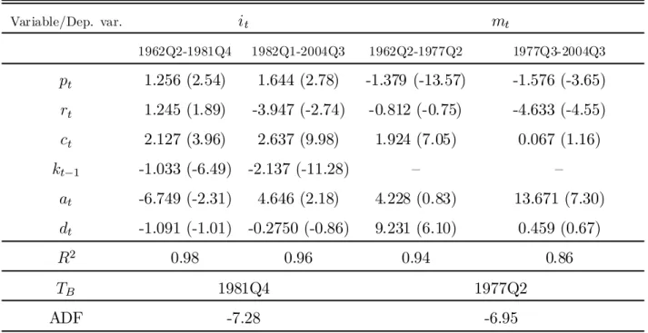
In Table 3, the ML results for it show that the coe¢cient of relative prices, pt, has

the opposite sign in both subperiods. Meanwhile, interest rates and the participation rate have the right signs during the most recent subperiod. Hence, rt and at are kept in the

speci…cation, whereas pt is removed. ML results from a restricted version are reported in

Table 4 and are discussed below.

4.1.2 Testing for symmetry in the speed of adjustment

In general, the adjustment mechanism in EqCM is assumed to be the same whether the innovations are positive or negative, or small or large. Granger and Lee (1989) introduce the notion of a non-symmetric equilibrium correction mechanism. The concept is simple. First, denote the innovations as "t ´ "+t +"¡t, so that "t is partitioned about zero into positive

and negative terms. To each resulting vector, n"+t

o

and n"¡t

o

, associate an adjustment parameter so that, for instance,±+ and±¡ can be estimated. While in (2) and (4) the sign of the innovation plays no role in determining the path of the adjustment (i.e., the adjustment is symmetric), by partitioning"tinto "+t and"¡t the joint hypotheses that±+ 6=±¡ and that

±+ _and _±¡ _{are both signi…cantly di¤erent from zero can be tested. For the non-symmetric} equilibrium correction model to be valid, Cook, Holly, and Turner (1999) argue that both hypotheses must be jointly veri…ed.

Non-symmetric equilibrium correction models have been used by Davidson et al. (1978) and by Cook, Holly, and Turner (1999) to explain consumption in the United Kingdom. Both studies conclude that consumption is adjusting asymmetrically to disequilibria.

Maximization of the likelihood function is attempted under the hypothesis that±+₁; ±¡₁; ±+₂; and ±¡₂ < 0, but ±+₁ is found to be (strongly) insigni…cant and ±+₂ is found to lie in an undesirable region, with a value of about -1:7. Under the assumption of stability, and given the information set used for the estimation, it can be concluded that the adjustment mechanism of the EqCMs models is better characterized as a symmetric process.8

(18)

4.1.3 Testing jointly for stability and symmetry

A natural extension of the robustness veri…cations performed above is to test jointly for the stability and symmetry hypotheses. To perform such a test, the estimated structural breaks are introduced in the long-run relations. Unfortunately, maximization of the likelihood func-tion is impossible, since some parameters cannot be identi…ed, causing a singularity. Overall, non-symmetric equilibrium correction does not seem to be admitted by this particular set of data, but the structural-change model, as discussed above, appears to provide signi…cant improvements over the usual hypothesis of linearity.

5 Selected Empirical Results

5.1 Assuming stable long-run relations

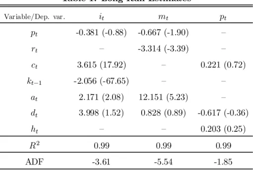
Table 1 reports empirical estimates for the long-run relations under the assumption of sta-bility. For (2), ®6 is restricted to zero, since the estimate obtained is slightly positive (but

not signi…cant), contrary to economic theory. While the null hypothesis of no cointegration can be rejected and relatively good estimates are obtained for the parameters of long-run relations involvingit andmt, it is not possible to …nd evidence of a decent long-run

relation-ship between prices and fundamental factors such as permanent income, demographics, and the level of activity in housing investment. This suggests that the price side of the housing market is e¢cient (i.e., unpredictable) in the long run, probably because the housing supply matches demand in the long run, so that fundamental (demand) factors have no permanent e¤ect on relative prices. Because there is a lack of evidence in favour of cointegration be-tween pt and its potential long-run determinants, the estimates for it and mt are based on

the results of a restricted version of the system, where only (7) determines the evolution of pt. For this reason, the short-run estimates, reported in Table 2, are based on the estimation

of the restricted system.

Forit, the ML estimates indicate that an increase in permanent income, demography, and

the participation rate have a positive e¤ect on investment in construction, while prices and stocks have a negative e¤ect, as expected. For resale volumes, both the participation rate and demography have a positive e¤ect, and prices and interest rates have a negative e¤ect, as expected. Although the t-statistics are rather low for some explanatory variables, these variables are kept in the speci…cation because economic theory suggests that they should be, and because their estimated parameters have the expected sign. Contrary to McCarthy and Peach (2004), we do not introduce the constraint that ®2 = -®4. This restriction imposes

(19)

a constant equilibrium between housing stocks and wealth. As the results suggest, this equilibrium is not supported by the Canadian data, since ®2 is about 75 per cent greater (in

magnitude) than ®4 and is tightly estimated.

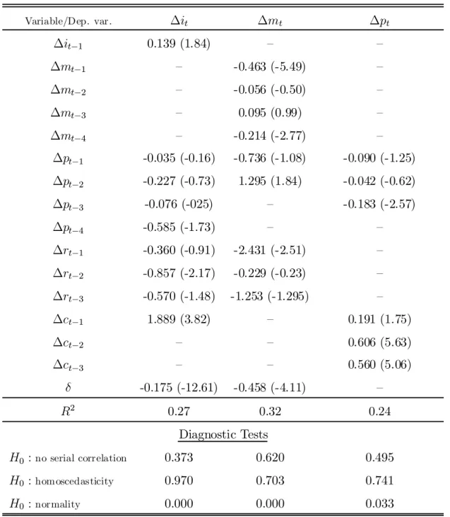
For the short-run parameter estimates, the ML estimates are qualitatively good, but the R2_{s are moderate, hovering around 0.3. While} _i

t adjusts to the disequilibrium at a

decent speed, with an estimated coe¢cient of adjustment of -0:175, mt adjusts more than

twice as fast with a coe¢cient of -0:458. The large di¤erence between the estimated speeds

of adjustment con…rms a priori expectations that modelling of housing investment data separately in two distinct categories permits a better understanding of how the housing sector operates. The empirical results suggest that adjustment costs are much lower in the resale market than in the construction market.

For the conditional persistence,¢itexhibits very little inertia, judging by its lower sum of

AR coe¢cients. The results for¢mt show a sum of AR coe¢cients of about -0:63, re‡ecting

the exceptional volatility of this series. The short-run response of it to changes in relative

prices is systematically negative; the maximum impact is felt after four lags. The cumulative impact onmt is at …rst negative and becomes positive only after 2 quarters. Shocks from

rt have a negative impact in the short run, with mt having the greater responsiveness. For

permanent income, the short-run e¤ects occur with only a single lag and are signi…cant only forit.

The short-run speci…cation for¢ptreveals that permanent income is the only explanatory

variable that signi…cantly a¤ects relative prices. The calculated long-run response of ¢pt is

roughly one for one.

5.2 Assuming unstable long-run relations

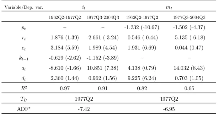
When a structural change is introduced in the long-run speci…cations, large shifts are found in the vector of population parameters.9 _{Compared with the base-case results noted earlier} (Table 1), evidence in favour of cointegration becomes more apparent (Table 4).10 _The impact of rt on it is interesting: an increase of 100 basis points in interest rates generates a

decrease of about 2.6 per cent in construction investment. The long-run response ofmt tort

is nearly twice that of the base-case estimate. These results suggest that the response of mt

to rt has increased substantially relative to the 1960s and 1970s. For the response of it to

ct, the estimates obtained under the hypothesis of a change in the long-run relation reveal

9_{Large shifts in the intercepts are also found, but those results are not shown.}

10_{Because the critical values tabulated in GH (1996a) are printed only up to (}_b₌_{) 4 stochastic explanatory}

(20)

that a 1 per cent increase in permanent income translates into about a 2 per cent increase in investment in construction, slightly more than the base-case estimate suggests. For mt,

the response to ct is virtually zero during the most recent period; this marks an important

drop compared with the results from before 1977. For the response to the changes in the participation rate, it increases by about 10 per cent when at rises by one percentage point

during the most recent subperiod, compared with only 2.1 per cent when there is no break. For mt, the response to variations inat increases threefold after the break to stand at about

14, and is roughly the same as the base-case estimates. The stock-adjustment e¤ects are just above one in the most recent period, nearly twice the e¤ect as before 1977 and half the e¤ect of the base-case estimate.

5.3 Short-run estimates

Based on the preferred long-run estimates, Table 5 reports the associated ML estimates for the dynamic speci…cations.11 _{Note the strength of the adjustment to the disequilibrium,} which increases substantially once a break in the cointegrating vectors is allowed for. This is shown by the estimated speed of adjustments, the^_±_{’s, and their associated}_t_{-statistics, which}

are consistently stronger than in the base-case estimates reported in Table 2. There are no other notable changes to the speci…cation of ¢it. Regarding ¢mt, note that the e¤ect of

relative prices becomes strictly negative. The quality of adjustment for both ¢it and ¢mt

improve overall, judging by the higher R2s.

Regarding the behaviour of the residuals, Lagrange-Multiplier (LM) tests for the null hypothesis of no serial correlation and for homoscedasticity; there is no evidence of serial dependence or conditional heteroscedasticity. Innovations from¢itand¢mtequations,

how-ever, appear to depart from normality, because of massive excess kurtosis, reaching 4.9 and 7.2, respectively. Although the validity of ML estimates depends upon the assumption that the processes are conditionally normal, Gonzalo (1994) shows that ML estimates speci…ed in error-correction models are superior to popular alternative estimation methods such as ordinary least squares. To address thoroughly the issue of non-normality, other types of non-linear functional forms would have to be investigated, which is beyond the scope of this paper. The empirical results in this paper can therefore be treated as quasi-ML estimates.

Since no changes are made to the speci…cation for ¢pt, the estimated function for it is

virtually unchanged relative to the system’s benchmark speci…cation.

11_{Recall that, although the long-run relations are allowed to shift over time, the short-run relations are}

(21)

5.4 Estimated equilibrium levels

Figures 3 and 4 compare the long-run equilibrium levels (the …t) suggested by the speci…-cations with (using the restricted model) and without breaks for both it and mt. A clear

improvement is observed in the …t by allowing for a structural break in the relations. In Figure 3, the structural-change model suggests that the level of investment in construction was very close to equilibrium during the 2003–04 period, while the base-case model signals an overshooting in investment by nearly 15 per cent in 2004Q2. Similarly, the peak in the late 1980s is explained by the structural-change model but not by the base-case model.

The base-case model suggests that the current housing market could su¤er from a rection and also suggests that investment levels should be brought down by the simple cor-rection mechanics of the disequilibrium component. The structural-change model, however, suggests that, as long as fundamentals remain strong, housing investment levels will remain high. Since the proposed empirical model cannot relate housing investment activity directly with housing prices, it is di¢cult to predict the outcome of prices if investment levels were to retreat signi…cantly.

Regarding the …t obtained for mt, neither speci…cation gives a clear explanation of the

many important and abrupt changes observed in this series. To a large extent, the …ts are not very di¤erent. Given the empirical results, this side of the housing market seems to have overheated in 2004.

6 Historical Decomposition of Housing Investment and Impulse Response 6.1 Historical decomposition

Figures 5 and 6 show the contributions of the explanatory variables to the level of activity for both sides of the housing market, as derived from the cointegrating relations. These contributions are also computed for the base-case linear models, so that the base-case results can be compared with those of the preferred structural-change model. The purpose of this exercise is strictly to compare how the di¤erent explanatory variables help to explain historical episodes in it andmt. To simplify this graphical analysis, the contributions from

the structural-change models are normalized within each subsample, but one should bear in mind that the estimated shifts in population parameters also imply large level realignments in the respective contributions. Hence, by applying a subsample normalization scheme, the shifts are removed so that emphasis is easily put on variations.

The decomposition of it in Figure 5 shows that permanent income, or wealth, provides a

(22)

put downward pressure on the activity level. Relative prices play a similar role in containing housing investment, in light of the fact that housing has steadily become more expensive over time relative to the cost of renting. The contribution of the demographic factor, dt,

is not always in line with the evolution of the construction market. For instance, there are long periods where its contribution clearly coincides with that of the investment cycle (e.g., 1970–95). In shorter periods, however, there is a sharp disconnect between the two, such as the 1995–2004 period when, according to the model, demography clearly pushed down housing demand while the solid expansion of the housing market was occurring. The contribution from the evolution of the participation rate, at, is interesting, particularly for

the structural-change model. The model suggests that, since the timing of the structural break in 1977, ‡uctuations in investment in construction have been partially induced by the participation rate. The contribution of interest rates follows the investment cycle closely, as expected.

For the contribution to the resale market (Figure 6), the greater volatility of the series is not easily explained by the proposed linear and structural-change models. While the demographic and wealth factors a¤ect mt and it similarly, the many sharp swings in the

resale data are not well explained by the models. Most notable in Figure 6 is the great volatility that interest rates induce in the resale market.

6.1.1 Growth accounting: understanding the 2001–04 trend

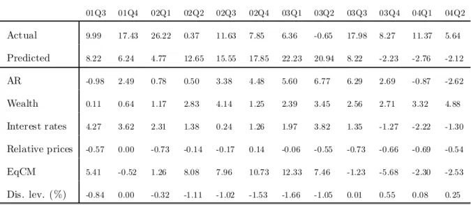
Table 6 reports the recent (2001Q3–2004Q2) contributions to growth for ht; given the

pre-ferred structural model, which includes a shift in the cointegrating vectors ofmtandit. The

contributions are obtained from a dynamic forecast of the system starting in 2001Q1. The predicted level of disequilibrium, expressed as a percentage of ht, is also tabulated over the

forecast exercise, as well as the actual and predicted growth of housing investment, expressed at annual rates.

According to the preferred model, wealth e¤ects have contributed steadily to support housing investment, whereas real interest rates did so only until late 2003. On the other hand, the continued relative appreciation of houses has muted growth over that period. Disequilibrium e¤ects contributed to boost growth until the middle of 2003, but as the housing market continued its expansion to the point of a slight overinvestment, it has been a drag on growth over the 2003Q3–2004Q2 period.

(23)

6.2 Impulse-response functions

This section summarizes the impulse-response functions (IRFs) embodied in the preferred structural model. The system-based IRFs are computed for ht by simulating the system

with and without shocks.

Figures 7 and 8 plot the calculated impact on the level of housing investment, which allows us to evaluate the long-run impacts. Most of the adjustment operates within a period of about 10 quarters. During the initial quarters (i.e., less than 2 years), the impact is quite large. For most IRFs, however, there is evidence of slight overshooting, as shown by the IRF’s hump-shape. The stock-adjustment e¤ect is part of the reason why the shock does not completely stabilize after 10 years: any shock toit causes a change in kt; while k¤t need

not change.

By considering the adjustment after a period of about 10 years, it can be seen that the impact of a 1 percentage point increase in wealth is just below one (Figure 7), which implies that, in the long run, the share of housing investment to wealth is constant. The impact of an increase of 100 basis points in the real mortgage interest rate translates into a peak response of about -2.5 per cent, before converging to -2 per cent (Figure 7). In the long run, a 1 percentage point increase in the participation rate translates into about a 7 per cent increase in ht (Figure 7). A 1 percentage point increase in the demographic variable results

in an increase inhtof slightly above half a per cent (Figure 8). A 1 percentage point increase

in the relative price of housing, however, causes a drop in ht of 0.2 per cent (Figure 8). 7 Models of the Housing Sector: A Leading-Indicator Approach

Apart from the national accounts data on housing investment, the housing sector is tracked by monthly and quarterly indicators, such as building permits and housing starts. They would be expected to be closely related to national accounts data on housing investment, particularly to the construction component. Building permits, issued by municipalities, are the …rst clear signal regarding future housing investment. After they are issued, it usually takes less than three months for building permits to translate into housing starts. Once work on a house has begun, the value of the expenditures is usually spread over a period of one to three months—somewhat more for multiple-unit housing projects.

Other indicators relevant to this study include credit market or labour market conditions, the price of housing, income, and/or consumer con…dence. These indicators may convey some short-run information about housing investment, particularly for the current or next 1 or 2 quarters. Hence, the main concern is to determine whether reliable LIs exist to predict

(24)

near-term developments in the housing sector.

This section therefore reports the estimation results from potential autoregressive leading-indicator (ARLI) models of housing. ARLI models are simply de…ned as follows (intercept omitted): xt= jx X j=1 Á_j¢xt¡j + jw X j=1 ¯_j¢wl;t¡j+et; (8)

where xt represents a variable of interest, xt =fit; mt;fht = it +mtgg0; wl;t represents the

l’th leading indicator; and et is white noise.12 The lags jx and jw are selected using the

Akaike information criterion, with a maximum of six lags. ARLI models are also estimated for the aggregate housing investment,ht, to determine whether there are advantages to using

disaggregate ARLI models over aggregate ones.

Other interesting LIs for the housing sector are the debt ratio and labour market indi-cators, such as employment growth and the unemployment rate. These indicators and all other housing market indicators that are analyzed in this study are listed in Appendix A. Forecasts from 14 di¤erent indicators are thus compared.

All LI variables are rendered stationary by means of appropriate di¤erentiation.

7.1 Empirical results

Table 7 reports the regression results for the aggregate measure,ht, using data from 1983Q3

to 2004Q3.13 _{According to the least squares-estimates and the calculated}_R2_{s, housing starts,}

building permits, and consumer con…dence (good time for major outlay) are the top three models; 60 per cent of the variance in growth in total housing investment is explained by these simple models. The results from the ARLI model suggest that a one per cent increase in the growth rate of housing starts will translate into a long-run increase of housing investment of around 0.4 per cent. Not surprisingly, a similar impact can be obtained from the permits directly. The weakest LI variable is the real disposable income, with a moderate R2 _of

about 28 per cent. Interestingly, however, the results from the ARLI model suggest that real disposable income andhtmove one for one in the long run. In terms of parameter estimates,

the other noteworthy empirical result is the debt ratio, for which a long-run response of nearly one for one is estimated.

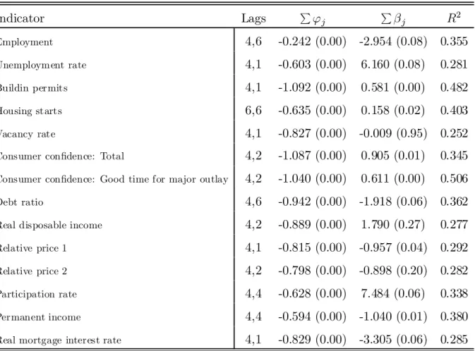
With respect to the growth of investment in construction,it, for which results are reported

in Table 8, the LI properties of housing starts and building permits are clearly revealed, as 12_{Because the main objective is to model investment ‡ows, the LI analysis does not extend to prices.}

Furthermore, the LI equations are assumed to remain constant over time, unlike the structural models.

13_{Although data are available from 1982Q1, the sample was trimmed by 6 quarters (i.e., the maximum}

(25)

would be expected given their relationship with construction. For housing starts, the R2

even approaches a full 80 per cent. Again, the explanatory power of real disposable income is comparatively low. The other results are comparable to the case where ht is directly

modelled.

The empirical results for mt, reported in Table 9, illustrate the volatile behaviour of the

resale market data. It is important to highlight in Table 9 the size of P'_j, which often approaches -1, and, in some cases, is even smaller than -1. This reveals the complexity of the dynamics that govern the volatile resale market. For the ARLI models, consumer con…dence (good time for major outlays) ranks …rst with an R2 _{of roughly 50 per cent, but building}

permits provide comparable information about the future of the resale market.

Although the sample period considered for the ARLI model is di¤erent from the one used for the structural models, the usefulness of ARLI models to predict the housing sector in the near term is promising, as expected. The in-sample evaluation performed above shows that ARLI models can explain a larger proportion of the historical variations of the housing sector.

8 Out-of-Sample Forecasts: Accuracy Comparison

In this section, the structural models’ out-of-sample forecast accuracy is analyzed, to deter-mine whether they can outperform simple ARLI models. The consequences of imposing the stability hypothesis on the structural models are also evaluated, as well as the usefulness of disaggregating housing investment data into the construction and resale categories when forecasting with ARLI models. The structural models are estimated using the full sample, whereas the indicator models are estimated using data only from 1983Q3. For the purpose of this forecasting exercise, all exogenous variables are considered as known over the fore-casting horizons. It should be remembered that the housing stock, kt, is also updated in the

forecasting exercise, according to (1).

The mean squared forecast error (MSFE) is simply calculated as(P _¡s)¡1PP

t=1e2t, where

P is the number of forecast errors and s is the forecast horizon.14 _P _{is set to 40 such that} there are su¢cient degrees of freedom during the second subsample to estimate £; and s is calculated for up to 8 quarters ahead. Our main concern is for one- and two-step-ahead forecasts.

(26)

8.1 Empirical results

Tables 10 to 12 report the MSFEs for the ARLI models, whereas Table 13 reports the MSFEs for the structural models under the hypothesis of both long-run stability and instability.

At one step ahead, the best ARLI forecast for aggregate housing investment, ht, is

ob-tained from the housing starts with a calculated MSFE of only 3.882. In comparison, the structural models that generate MSFEs are similar whether a break is included or not (5.9 when no break is included and 6 otherwise). Nonetheless, the MSFE from the best ARLI model is nearly half that of the best structural model. Also note that only 4 of the 14 ARLI models provide a lower MSFE than the structural models (one step ahead).

Similarly, for it, we …nd that ARLI models that make use of housing-starts data

out-perform the best structural model by reducing the one-step-ahead MSFE by about 35 per cent.15 _{Interestingly, for} _i

t, allowing for a break improves the forecast accuracy of the

struc-tural model.

For the resale market, ARLI and structural models provide very comparable forecasts at one step ahead, whereas for longer horizons the relative forecast performance of the structural models deteriorates dramatically. In e¤ect, the best one-step-ahead MSFE for the ARLI class of models is obtained by building permits, followed closely by consumer con…dence (good time for major outlay). While the structural models’ forecasts for ht are very similar, it

appears that the di¢culties of the model that experiences a break in predicting mt are

outweighed by that model’s ability to predictit.

To predict near-term developments in the housing sector, whether in the aggregate or in components, simple LI models are relatively accurate. One of the reasons for the relatively poor performance of the structural models is that they require many parameters to be estimated, thereby increasing the MSFE. While aggregate housing investment (ht) is best

predicted by ARLI models, the results show that the preferred structural model provides very competitive forecasts for the construction category (it), whereas the accuracy for the

resale category (mt) is disappointing.

In contrast to the ARLI models, the structural models reveal the sources of the movements in housing investment and hence in housing starts and building permits. They also reveal whether the level of housing investment is consistent with fundamentals and therefore subject to future correction.

15_{Because data on housing starts can be separated into the} _singles _and_multiples _{categories, the forecast}

performance of an ARLI model that uses both subcategories is also examined, but we …nd that this approach does not help improve the forecast accuracy over using only the aggregate housing-starts series.

(27)

9 Conclusion

To explain housing investment, we have proposed multivariate speci…cations that model the joint process of housing investment and prices and exploit the long-run relationships between housing investment and fundamental factors. The preferred speci…cations allow for a structural change to a¤ect the cointegrating vectors for housing investment. The empirical results show that fundamental information helps explain variations in housing investment, in both the long and short run. We could not, however, …nd a valid long-run relationship that links the relative price of housing to fundamental variables. Growth of relative housing prices can only be explained by the evolution of wealth.

With respect to the out-of-sample forecast performance, the most accurate approach is provided by a LI model that uses building permits or housing starts. Although this result is not surprising, given the accounting relationship between national accounts’ housing investment and housing starts, it is interesting that the preferred structural model with a structural break ranks better than each of the 12 LI models of construction investment.

Although the empirical …ndings do not permit speculation on the future of housing prices, the results suggest that fundamental factors seem to support the high investment levels ob-served since 2000. This con…rms the view that the housing sector is not driven by speculative behaviour.

While interesting results have been obtained for the construction component of housing investment, the resale component has proven to be di¢cult to model successfully. An in-teresting avenue for future research would be to examine the possibility of threshold e¤ects associated with mortgage rates. Similarly, functional forms that are more ‡exible could prove useful.

(28)

References

Berger-Thomson, L. and L. Ellis. 2004. “Housing Construction Cycles and Interest Rates.” Reserve Bank of Australia, Research Discussion Paper 2004–08.

Case, K.E. and R.J. Shiller. 1990. “Forecasting Prices and Excess Return in the Housing Market.” AREUEA Journal 2: 1–20.

Cook, S., S. Holly, and P. Turner. 1999. “DHSY Revisited: The Role of Asymmetries.”

Applied Economics 31: 775–8.

Davidson, J.E., D.F. Hendry, F. Srba, and S. Yeo. 1978. “Econometric Modelling of the Aggregate Time Series Relationship Between Consumers’ Expenditure and Income in the United Kingdom.” Economic Journal 88: 661–92.

DiPasquale, D. 1999. “Why Don’t We Know More About Housing Supply?” Journal of Real Estate Finance and Economics 18: 9–24.

DiPasquale, D. and W. Wheaton. 1994. “Housing Market Dynamics and the Future of Housing Prices.” Journal of Urban Economics 35: 1–27.

Egebo, T., P. Richardson, and I. Lienert. 1990. “Modèles de l’investissement résidentiel pour les grands pays de l’OCDE.” Revue économique de l’OCDE 14: 165–207.

Engelhardt, G.V. and J.M. Poterba. 1991. “House Prices and Demographic Change.”

Regional Science and Urban Economics 21: 539–46.

Engle, R.F. and C.W.J. Granger. 1987. “Co-integration and Error Correction: Represen-tation, Estimation, and Testing.” Econometrica 55: 251–76.

Engsted, T. and N. Haldrup. 1999. “Multicointegration in Stock-Flow Models.” Oxford Bulletin of Economics and Statistics 61: 237–54.

Fair, R.C. 1972. “Disequilibrium in Housing Models.” Journal of Finance 2: 207–21. Friedman, M. 1957. A Theory of the Consumption Function. Princeton: Princeton

Univer-sity Press.

Gonzalo, J. 1994. “Five Alternative Methods of Estimating Long Run Equilibrium Rela-tionships.” Journal of Econometrics 60: 203–33.

(29)

Granger, C.W.J. and T.H. Lee. 1989. “Investigation of Production, Sales and Inventory Relationships Using Multicointegration and Non-symmetric Error Correction Models.”

Journal of Applied Econometrics 4: 145–59.

Gregory, A.W. and B.E. Hansen (GH). 1996a. “Residual-based Tests for Cointegration in Models with Regime Shifts.” Journal of Econometrics 70: 99–126.

. 1996b. “Tests for Cointegration in Models with Regime and Trend Shifts.”

Oxford Bulletin of Economics and Statistics 58: 555–60.

Gregory, A.W., J. Nason, and P.G. Watt. 1996. “Testing for Cointegration in Models with Regime Shifts.” Journal of Econometrics 71: 321–41.

Haldrup, N. 1994. “The Asymptotics of Single-Equation Cointegration Regressions with I(1) and I(2) Variables.” Journal of Econometrics 63: 153–81.

Hanushek, E.A. and J.M. Quigley. 1979. “The Dynamics of the Housing Market: A Stock Adjustment Model of Housing Consumption.” Journal of Urban Economics6: 90–111. . 1982. “The Determinants of Housing Demand.” Research in Urban Economics

2: 221–42.

Johansen, S. 1991. “Estimation and Hypothesis Testing of Cointegration Vectors in Gaussian Vector Autoregressive Models.” Econometrica 59: 1551–80.

Kostenbauer, K. 2001. “La dépréciaition du logement dans l’IPC canadien.” Statisitics Canada, No. 62F0014MIF, Série No. 15.

Krainer, J. 2005. “Housing Markets and Demographics.” Federal Reserve Bank of San Francisco,FRBSF Economic Letter 27, October 1.

Krainer, J. and C. Wei. 2004. “House Prices and Fundamental Value.” Federal Reserve Bank of San Francisco,FRBSF Economic Letter 21, August 26.

Macklem, T. 1994. Wealth, Disposable Income and Consumption: Some Evidence for Canada. Technical Report No. 71. Ottawa: Bank of Canada.

. 2001. “A New Measure of Core In‡ation.” Bank of Canada Review (Autumn): 3–12.

(30)

Malpezzi, S. and D. Maclennan. 2001. “The Long-Run Price Elasticity of Supply of New Residential Construction in the United States and the United Kingdom.” Journal of Housing Economics 10: 278–306.

Mankiw, G. and D.N. Weil. 1989. “The Baby Boom, the Baby Bust, and the Housing Market.” Regional Science and Urban Economics 19: 235–58.

McCarthy, J. and R.W. Peach. 2002. “Monetary Policy Transmission to Residential Invest-ment.” Federal Reserve Bank of New York, Economic Policy Review (May): 139–58.

. 2004. “Are Home Prices the Next Bubble?” Federal Reserve Bank of New York,Economic Policy Review (December): 1–17.

Palumbo, M., J. Rudd, and K. Whelan. 2002. “On the Relationship Between Real Con-sumption, Income, and Wealth.” Federal Reserve Board. Photocopy.

Phillips, P.C.B. and S. Ouliaris. 1990. “Asymptotic Properties of Residual Based Tests for Cointegration.” Econometrica 58: 165–93.

Riddel, M. 2004. “Housing-Market Disequilibrium: An Examination of Housing-Market Prices and Stock Dynamics 1967-1998.” Journal of Housing Economics 12: 120–35.

(31)

Table 1: Long-Run Estimates Variable/Dep. var. it mt pt pt -0.381 (-0.88) -0.667 (-1.90) – rt – -3.314 (-3.39) – ct 3.615 (17.92) – 0.221 (0.72) kt¡1 -2.056 (-67.65) – – at 2.171 (2.08) 12.151 (5.23) – dt 3.998 (1.52) 0.828 (0.89) -0.617 (-0.36) ht – – 0.203 (0.25) R2 0.99 0.99 0.99 ADF -3.61 -5.54 -1.85

Note: p-values are in parentheses. Sample period: 1962Q1–2004Q3. For the ADF tests, the Phillips & Ouliaris (1990, Table IIb) 10 per cent critical values are: b=3, -3.83;b=4, -4.16;b=5, -4.43, wherebis the number of stochastic regressors included in a long-run relation.

(32)

Table 2: Short-Run Estimates Variable/Dep. var. ¢it ¢mt ¢pt ¢it¡1 0.139 (1.84) – – ¢mt_¡1 – -0.463 (-5.49) – ¢mt_¡2 – -0.056 (-0.50) – ¢mt¡3 – 0.095 (0.99) – ¢mt_¡4 – -0.214 (-2.77) – ¢pt_¡1 -0.035 (-0.16) -0.736 (-1.08) -0.090 (-1.25) ¢pt¡2 -0.227 (-0.73) 1.295 (1.84) -0.042 (-0.62) ¢pt_¡3 -0.076 (-025) – -0.183 (-2.57) ¢pt¡4 -0.585 (-1.73) – – ¢rt_¡1 -0.360 (-0.91) -2.431 (-2.51) – ¢rt_¡2 -0.857 (-2.17) -0.229 (-0.23) – ¢rt¡3 -0.570 (-1.48) -1.253 (-1.295) – ¢ct_¡1 1.889 (3.82) – 0.191 (1.75) ¢ct¡2 – – 0.606 (5.63) ¢ct_¡3 – – 0.560 (5.06) ± -0.175 (-12.61) -0.458 (-4.11) – R2 _0.27 _0.32 _0.24 Diagnostic Tests H0:no serial correlation 0.373 0.620 0.495 H0:homoscedasticity 0.970 0.703 0.741 H0:normality 0.000 0.000 0.033

Note: p-values are in parentheses. Sample period: 1962Q1–2004Q3. For the diagnostic tests, thep-values are reported. The LM tests are performed for order 2 processes.

(33)

Table 3: Long-Run ML Estimates With Break (Unrestricted) Variable/Dep. var. it mt 1962Q2-1981Q4 1982Q1-2004Q3 1962Q2-1977Q2 1977Q3-2004Q3 pt 1.256 (2.54) 1.644 (2.78) -1.379 (-13.57) -1.576 (-3.65) rt 1.245 (1.89) -3.947 (-2.74) -0.812 (-0.75) -4.633 (-4.55) ct 2.127 (3.96) 2.637 (9.98) 1.924 (7.05) 0.067 (1.16) kt_¡1 -1.033 (-6.49) -2.137 (-11.28) – – at -6.749 (-2.31) 4.646 (2.18) 4.228 (0.83) 13.671 (7.30) dt -1.091 (-1.01) -0.2750 (-0.86) 9.231 (6.10) 0.459 (0.67) R2 _0.98 _0.96 _0.94 _0.86 TB 1981Q4 1977Q2 ADF -7.28 -6.95

Note: p-values are in parentheses. Sample period: 1962Q1–2004Q3. TB is the estimated break point. For

the ADF tests, the 10 per cent critical values, simulated usingT=150 and 1,000 replications, are: b=5, -6.62;b=6, -7.03, whereb is the number of stochastic regressors included in a long-run relation.

(34)

Table 4: Long-Run ML Estimates With Break (Restricted) Variable/Dep. var. it mt 1962Q2-1977Q2 1977Q3-2004Q3 1962Q2-1977Q2 1977Q3-2004Q3 pt – – -1.332 (-10.67) -1.502 (-4.37) rt 1.876 (1.39) -2.661 (-3.24) -0.546 (-0.44) -5.135 (-6.18) ct 3.184 (5.59) 1.989 (4.54) 1.931 (6.69) 0.044 (0.47) kt_¡1 -0.629 (-2.62) -1.152 (-3.89) – – at -8.610 (-1.66) 10.851 (7.38) 4.138 (0.79) 14.032 (8.43) dt 2.360 (1.44) 0.962 (1.56) 9.225 (6.24) 0.703 (1.05) R2 _0.97 _0.91 _0.82 _0.65 TB 1977Q2 1977Q2 ADF¤ _-7.42 _-6.95

Note: p-values are in parentheses. Sample period: 1962Q1–2004Q3. TB is the estimated break point.

For the ADF tests, the 10 per cent critical values, simulated usingT=150 and 1,000 replications, are: b=5, -6.62, whereb is the number of stochastic regressors included in a long-run relation.

(35)

Table 5: Short-Run Estimates From Restricted Long-Run Models Variable/Dep. var. ¢it ¢mt ¢pt ¢it¡1 0.086 (1.15) – – ¢it_¡2 -0.035 (-0.53) – – ¢it_¡3 0.137 (1.94) – – ¢it¡4 -0.134 (-1.98) – – ¢mt_¡1 – -0.607 (-8.17) – ¢mt_¡2 – 0.005 (0.14) – ¢mt¡3 – 0.126 (1.81) – ¢mt_¡4 – -0.159 (-2.58) – ¢pt¡1 -0.056 (-0.38) -1.202 (-1.86) -0.099 (-1.34) ¢pt_¡2 -0.242 (-0.80) – 0.006 (1.14) ¢pt_¡3 -0.136 (-0.47) – -0.185 (-2.60) ¢pt¡4 -0.285 (-0.87) – – ¢rt_¡1 -0.599 (-1.56) -2.865 (-2.96) – ¢rt¡2 -0.429 (-1.12) 0.421 (0.50) – ¢rt_¡3 -0.533 (-1.33) -0.947 (-1.00) – ¢ct_¡1 1.821 (4.08) – 0.142 (1.31) ¢ct¡2 – – 0.559 (5.19) ¢ct_¡3 – – 0.601 (5.49) ± -0.317 (-14.88) -0.713 (-15.13) – R2 _0.39 _0.34 _0.23 Diagnostic Tests H0: no serial correlation 0.370 0.439 0.458 H0: homoscedasticity 0.934 0.627 0.744 H0: normality 0.000 0.000 0.030

Note: p-values are in parentheses. Sample period: 1962Q1–2004Q3. For the diagnostic tests, p-values are reported. The LM tests are performed for order 2 processes.

(36)

Table 6: Contributions to Growth for ht (2001Q3–2004Q2) 01Q3 01Q4 02Q1 02Q2 02Q3 02Q4 03Q1 03Q2 03Q3 03Q4 04Q1 04Q2 Actual 9.99 17.43 26.22 0.37 11.63 7.85 6.36 -0.65 17.98 8.27 11.37 5.64 Predicted 8.22 6.24 4.77 12.65 15.55 17.85 22.23 20.94 8.22 -2.23 -2.76 -2.12 AR -0.98 2.49 0.78 0.50 3.38 4.48 5.60 6.77 6.29 2.69 -0.87 -2.62 Wealth 0.11 0.64 1.17 2.83 4.14 1.25 2.39 3.45 2.56 2.71 3.32 4.88 Interest rates 4.27 3.62 2.31 1.38 0.24 1.26 1.97 3.82 1.35 -1.27 -2.22 -1.30 Relative prices -0.57 0.00 -0.73 -0.14 -0.17 0.14 -0.06 -0.55 -0.73 -0.66 -0.69 -0.54 EqCM 5.41 -0.52 1.26 8.08 7.96 10.73 12.33 7.46 -1.23 -5.68 -2.30 -2.53 Dis. lev. (%) -0.84 0.00 -0.32 -1.11 -1.02 -1.53 -1.66 -1.05 0.01 0.55 0.08 0.25

(37)

Table 7: LI Models’ Estimation Results for ht (1983Q3–2004Q3) Indicator Lags P'j P¯j R2 Employment 4,5 0.429 (0.00) 0.935 (0.04) 0.403 Unemployment rate 5,1 0.488 (0.00) 0.559 (0.61) 0.330 Building permits 4,3 0.154 (0.04) 0.377 (0.00) 0.622 Housing starts 4,3 0.140 (0.02) 0.365 (0.00) 0.668 Vacancy rate 5,1 0.460 (0.00) -0.029 (0.51) 0.332

Consumer con…dence: Total 1,3 0.501 (0.00) 0.207 (0.00) 0.445

Consumer con…dence: Good time for ma jor outlay 5,2 0.570 (0.00) 0.200 (0.00) 0.552

Debt ratio 1,5 0.417 (0.00) -0.445 (0.05) 0.354

Real disposable income 1,1 0.491 (0.00) 0.519 (0.09) 0.284

Relative price 1 5,4 0.405 (0.00) -0.805 (0.09) 0.397

Relative price 2 5,1 0.426 (0.00) -0.296 (0.48) 0.332

Participation rate 1,5 0.568 (0.00) 1.418 (0.02) 0.380

Permanent income 5,3 0.443 (0.00) 0.756 (0.11) 0.380