Shale gas development and respiratory health

(1)

SHALE GAS DEVELOPMENT AND RESPIRATORY HEALTH

BY

SARAH ALLISON GRAJDURA

THESIS

Submitted in partial fulfillment of the requirements

for the degree of Master of Science in Agricultural and Applied Economics in the Graduate College of the

University of Illinois at Urbana-Champaign, 2016

Urbana, Illinois

Master’s Committee:

Professor Amy Ando, Co-Chair

Assistant Professor Erica Myers, Co-Chair Professor Madhu Khanna

(2)

ABSTRACT

Hydraulic fracturing, or “fracking” has rapidly increased in areas rich in shale gas and oil in the years 2006 onwards. Areas that have undergone shale gas development are likely to be largely rural with few other air pollution point sources. Fracking operations such as well drilling, gas processing, and increased truck traffic are all predicted to contribute to localized air pollution in areas where fracking has been intensifying. Using the natural experiment of the New York fracking ban and intensifying fracking in Northeastern Pennsylvania, oil and gas well data and state inpatient respiratory records are combined to estimate the effect of various levels of shale gas development on respiratory admissions. A border exclusion was applied to account for air pollution spillovers. We find that the presence of fracking wells affects elderly respiratory hospital admissions by increasing admission rates 16-31%, and the results are robust across different levels of fracking and border exclusions.

(3)

Hydraulic fracturing is a stimulation technique used to increase production of oil and gas by forcing fluids into the subsurface at high pressures, creating fractures that remain open after the injection is terminated (EPA 2015). The technologies of horizontal drilling and hydraulic fracturing have made natural gas and oil resources from low permeability geological formations, or “unconventional” geological formations, that were previously considered uneconomic to extract, now economically viable (EIA 2015). This change in availability of resources has been called the “Shale Revolution” in the United States. Oil and gas flow through these cracks and are subsequently extracted at the surface. In the past, this process was restricted to vertical wells but with technological improvements, this process can be applied to vertical, deviated, or

horizontal wells (EPA 2015). This process requires large volumes of water in addition to complex mixtures of water, proppants and chemicals, and is sometimes referred to as high volume hydraulic fracturing (HVHF). These new techniques spread to low-permeability formations across the country in 2005, making modern hydraulic fracturing the industry standard, driving the surge in U.S. production of natural gas (EPA 2015).

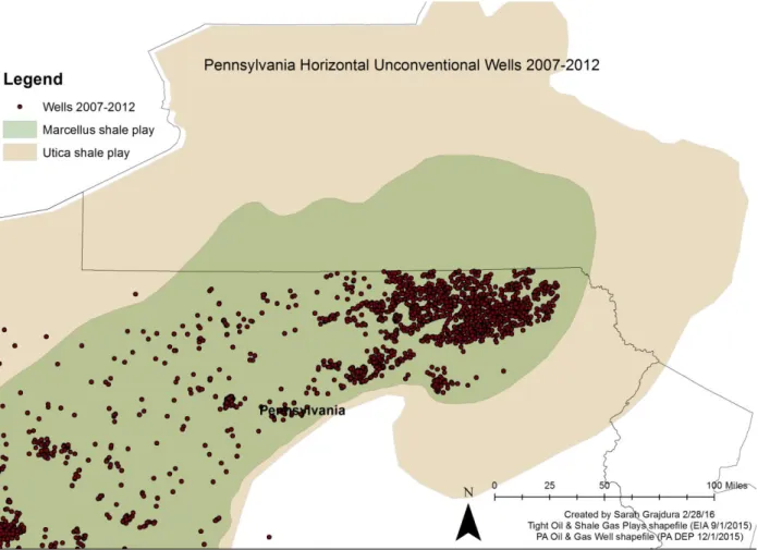
Shales are considered an “unconventional” geologic formation and are characterized by fine-grained sedimentary rock that forms from the compaction of silt and clay-size mineral particles and has the ability to trap natural gas and oil (EIA 2015). The types of resources found in low permeability formations include shale gas, tight gas, and tight oil. The Marcellus Shale is a shale play found primarily in Pennsylvania, New York, and West Virginia, as shown in Figure 1. The Utica Shale play lies below the Marcellus and underlies mainly New York, Pennsylvania, Ohio, and West Virginia, but also extends into Ontario, Quebec, Maryland, Tennessee, and

(5)

Virginia. Since 2012, the Marcellus and Utica shale plays have accounted for 85% of the increase in shale gas production in the U.S. (EIA 2015).

There is a growing body of research examining local effects of shale gas development on outcomes such as water use, air quality, and health, property values. In particular, it has been found that air pollution is higher near unconventional wells and natural gas processing equipment (Goetz et al. 2013; Rich et al. 2014), and health studies have suggested that air pollution may be the main vector responsible for increased birth effects near fracking wells (Hill 2013). However, fracking well distance and intensity has not been definitively linked to

respiratory health incidence. This paper examines whether there is indeed a link between intensifying fracking operations and respiratory health outcomes.

1.1LITERATURE REVIEW

Shale gas development generates several direct market benefits and positive externalities. Due to the large increase in supply caused by shale extraction, consumers have seen lower natural gas prices. This has increased consumer surplus by an estimated $4.36 billion from January 2007 to January 2014, or a monthly increase of $51.9 million per month (Mason 2015). Likewise, producers have benefitted from the increased value of reserve holdings coupled with the increased producer surplus caused by the increased availability of resources. This increase in producer surplus is estimated to be on the order of $9.60 billion from January 2007 to January 2014 (Mason 2015). Labor has also been shown to benefit from shale gas extraction, with increases in positive total employment (Cosgrove 2014; DeLeire et al. 2014; Komarek 2015). However, direct income effects where drilling occurs are found to be relatively small, at least in

(6)

the Marcellus region of Pennsylvania, likely due to drilling companies importing outside workers (DeLeire et al. 2014; Paredes 2015).

Likewise, several positive externalities have arisen from shale gas development. One positive externality is increased domestic energy stability, since the shale boom has altered the U.S.’s expected energy procurement trajectory by decreasing imports of oil and liquid natural gas (LNG). Furthermore, the low price of natural gas has driven substitution in electricity generation from coal to natural gas and in a smaller capacity from oil to natural gas in the

transportation sector (Mason 2015). Natural gas is a cleaner-burning fuel compared to coal or oil; hence, its use in electricity generation creates less CO2 emissions. Likewise, when burned,

natural gas does not emit such harmful pollutants like mercury, which adversely affect human health. LaReviere et. al attempt to quantify these climate benefits and health benefits in their manuscript “Quantifying Environmental Benefits of Fracking: The Decline of Coal, Air Quality and Asthma Rates.” People living downstream of a coal plant would likely to receive the largest benefits (LaRiviere et al. 2014).

1.2COSTS AND NEGATIVE EXTERNALITIES

Although natural gas is cleaner-burning than coal, the process of extracting shale gas is arguably more carbon intensive. Howarth et al. (2000) find that compared to coal, the footprint of shale gas is at least 20% greater and perhaps more than twice as great on the 20-year horizon and is comparable when compared over 100 years. These methane emissions are at least 30% and up to twice as great as emissions from conventional gas (Howarth et al. 2011). The possible negative externalities of fracking have been widely publicized and have even resulted in fracking bans in places like Denton, Texas and New York State. Surface water and groundwater resources

(7)

are at risk due hydraulic fracking operations. Depletion of rivers, streams, lakes, and

groundwater can occur when large withdrawals are made for fracking injection fluids. Pollution of surface water and groundwater is also possible through several mechanisms. Such pathways include spills during chemical and flowback water transport, well casing leaks (Kovats et al. 2014), runoff from drilling sites, underground leaks from fissures caused by fracking, and disposal of flowback fluids (Rozell & Reaven 2012; Rabinowitz et al. 2015).

There are several hedonic papers that examine the effect of shale gas development on housing values, mostly in the shale-rich regions of Colorado, Texas, Pennsylvania, and North Dakota. The first of such studies, by Boxall, et al. (2005) examined the impact of sour gas wells and flaring oil batteries in Alberta Canada. Subsequent studies have offered further insight into the housing and land impacts of oil and gas development. Bennett, et al. (2014) separates the effects of fracked wells on urban and rural housing values. Gopalakrishnan, et al. (2015) explore housing values in Pennsylvania and find heterogeneous effects of having additional shale well within one mile of a property. This paper along with others such as Muehlenbachs et al. (2012 & 2013) explore the difference in housing values across drinking sources. They find that

groundwater-dependent homes can have a reduced value of up to 24% (Muehlenbachs et al. 2012). The valuations of expectations of shale gas development, as capitalized in housing values, have also been examined by using the New York/Pennsylvania border discontinuity, and find that shale gas development is positively valued as indicated lower housing values in New York counties (Boslett et al. 2014). A contingent valuation survey in Texas and Florida showed a 5-15% reduction in bid values for homes located near fracking operations (Throupe et al. 2013).

Other externalities from shale gas development include habitat fragmentation (Northrup & Wittemyer 2013), increased rates of violent crimes (James & Smith 2014), potentially

(8)

decreased tourism (Parker & Phaneuf 2013), welfare losses to those living in fracking counties (Popkin et al. 2013), more deadly traffic accidents (Muehlenbachs & Krupnick 2014), smaller returns to education, and higher high school dropout rates (Cascio & Ayushi 2015).

1.3LOCAL AIR QUALITY, HEALTH, AND FRACKING

Despite these perceived climate and respiratory health benefits touted from coal substitution, there is cause for concern regarding air quality degradation for those living near hydraulic fracturing wells. Due to the clustered nature of fracking wells, extraction industry damages will not be constant over time or evenly distributed in space, so it is important to understand when and where damages occur (Litovitz et al. 2013). Although emissions for Pennsylvania as a whole are decreasing due to switching from coal to natural gas, rural areas are seeing higher emissions, due to few other point source pollution sources (Litovitz et al. 2013). As Schmidt (2011) points out, the EPA’s authority over air emissions from shale development is limited through the Clean Air Act, even though there is evidence that total fracking emissions from the shale development operations-drill rigs, condensate tanks, compressors, etc.-could generate enough emissions to qualify as a major source (Schmidt 2011). The 2009 Texas Barnett shale greenhouse gas emissions alone were estimated to be equivalent to the impact from two 750 MW coal-fired power plants (Armenderiz 2009).

It has been found that air pollution is higher near unconventional wells and natural gas processing equipment (Goetz et al. 2013; Rich et al. 2014). Utilizing natural gas from shale deposits produces air emissions of various types during extraction, transportation, and end use (Litovitz et al. 2013). High levels of emissions have been found near well pads, even when operators use a closed loop system and best management practices (Colborn et al. 2012). It is

(9)

estimated that 3.6% to 7.9% of the methane from a shale gas well escapes to atmosphere in venting and leaks over the lifetime of a well (Howarth et al. 2011). Pétron et al. (2012) identified mixing ratios of methane, benzene, and several other NMHCs to be caused by increased venting emissions (leaks) of raw natural gas and flashing emissions from condensate storage tanks in air masses affected by increased oil and gas operations in Garfield County, Colorado. Their results suggest that emissions of natural gas are greatly underestimated, possibly by as high as a factor of two (Pétron et al. 2012). The Garfield County community health risk analysis of the oil and gas industry that preceded the Pétron study recommended 24-hour sampling around the

perimeter of drill pads to achieve continuous monitoring throughout all stages of drilling (Coons & Walker 2008). In addition to these direct emissions, evaporation from on-site wastewater storage pits is also a pollution concern. In Pennsylvania, flowback fluids are not usually disposed of in deep injection wells, so these surface ponds are common (Rabinowitz et al. 2015).

More than 75% of the chemicals identified in fracking fluids and related emissions could affect the skin, eyes, and other sensory organs, and the respiratory and gastrointenstinal systems (Colborn et al. 2011). Direct pollutants include volatile organic chemicals (VOCs), nitrogen oxides (NOx), particulate matter (PM), sulfur dioxide (SO2), and carbon monoxide (CO). Direct

air quality measurements show high levels of non-methane hydrocarbons (NMHCs) during initial well drilling, as well as toxic levels of polycyclic hydrocarbons (PAHs); NMHC’s are associated with numerous endocrine disorders and are precursors of ozone (Colburn et al. 2012). Ozone (O3) is indirectly created by the combination of VOCs and NOx. Vehicular exhaust also

contains VOCs, so one might question whether increased truck traffic due to shale gas

development, or the shale gas extraction process itself is responsible for such emissions. Gilman et al. (2013) compare the raw natural gas source signature to VOC measurements in northeastern

(10)

Colorado, and find that the VOC source signature associated with oil and natural gas operations is clearly differentiated from other urban areas, which are dominated by vehicular exhaust. They estimate that on average 55+/18% of VOC-related ozone precursors are attributed to oil and natural gas operations (Gilman et al. 2013). SO2 and NOx exposure has been linked to adverse

respiratory effects, while exposure to PM and O3 would be expected to increase

respiratory-related hospital admissions, emergency room visits, and premature death (Litovitz et al. 2013). Litovitz et. al provide an estimate of air quality damages due to Marcellus shale natural gas extraction in Pennsylvania. They find that shale gas extraction is only a small percentage of total statewide emissions; however in counties where shale gas extraction is concentrated, NOx

emissions were 20-40 times higher than allowable for a single minor source (Litovitz et. al 2013). McKenzie et. al. estimate chronic and subchronic non-cancer indices and cancer risks for exposures to air emissions from the extraction of unconventional natural gas resources in

Colorado. They find that residents living within half a mile of wells are at greater risk for health effects than those living beyond half a mile from wells (McKenzie et al. 2012).

The literature demonstrating shale gas development’s direct effects on human or animal health is smaller. Bamberger & Oswald (2012) qualitatively interview farmers residing near fracking wells regarding livestock health, and document numerous health effects that coincide with water and air pollution events (flaring of well, storm water runoff from well pad,

compressor station malfunction, well/spring water intrusion, etc.). No causal links can be made from this study, however, due to the incomplete testing and disclosure of chemicals, and nondisclosure agreements (Bamberger & Oswald 2012). McKenzie et al. (2014) find an association between the density of unconventional gas wells, maternal residence, and the prevalence of various birth defects in rural Colorado (McKenzie et al. 2014). Likewise, Hill

(11)

(2012) examines birth outcomes of mothers living near unconventional wells in Pennsylvania. They find that that mothers living within 2.5 km of an unconventional well experience several adverse birth outcomes at higher levels, including a 25% increase in low birth weight. An important finding of this paper is that when Hill controls for differing water sources (piped water vs. well water), the change in estimates is not statistically significant, which suggests that the exposure mechanism is likely air pollution or increased economic activity (increased noise, stress from community change) (Hill 2013). Furthermore, in their random-sample healthy symptom survey of 492 persons in Washington County, Pennsylvania, Rabinowitz et al. (2015) find upper respiratory symptoms to be more frequently reported in persons living in households within 1 km from gas wells (39%) as compared to 1-2 km (31%) and > 2km (18%). These findings motivate the research goal of this paper, which is to quantify the effect of shale gas development, via air pollution, on respiratory health. Several of the aforementioned studies have indicated a need for better air quality monitoring and research on air quality near natural gas operations (Colburn et al. 2012; Pétron et al. 2012; McKenzie et al. 2012; McKenzie et al. 2014; Coons & Walker 2008; Bamberger & Oswald 2012; Rabinowitz et al. 2015; Meng 2014).

The aforementioned literature consists of case studies, health impact assessments, and toxicology reports, but does not include any empirical evidence relating respiratory health to fracking. Public health literature suggests that human health is affected, but nothing rigorous has been presented. This paper fills this gap by conducting an empirical analysis of the effects of proximity and intensity of fracking activities on human respiratory health. Respiratory health will be measured by respiratory ailment hospitalizations per capita. This question is important because as fracking expands throughout the U.S., China, and Eastern Europe, it is necessary to

(12)

better understand its health effects. To date, there have been no empirical studies showing the impact, if any, of shale gas development on respiratory health.

(13)

2. METHODS 2.1STUDY AREA

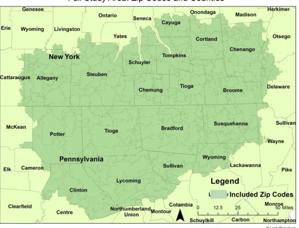
This study focuses on Northeastern Pennsylvania, which lies above the Marcellus and Utica shale plays. This region of Pennsylvania has experienced an exponential increase in fracking from 2007-2012. However, across the border in New York where there is equal shale potential, there has been a fracking moratorium in place since July 2006, which turned into an outright ban in December 2014. The high rate of fracking in Pennsylvania and lack of fracking in New York makes this an ideal region for a natural experiment studying the effects of fracking. This region comprising Northeastern Pennsylvania and Southeastern New York is largely rural, and residents on either side of the border largely supported fracking in its infancy due to the possibility of lucrative land leases. The full study area consists of 297 zip codes in total, 173 New York zip codes and 124 Pennsylvania zip codes, as shown in Figure 3. The Pennsylvania zip codes largely fall within the counties of Bradford, Clinton, Lycoming, Potter, Sullivan, Susquehanna, Tioga, and Wyoming. The New York zip codes are located mainly in Allegany, Steuben, Schuyler, Chemung, Tompkins, Cortland, Tioga, Broome, and Chenango counties.

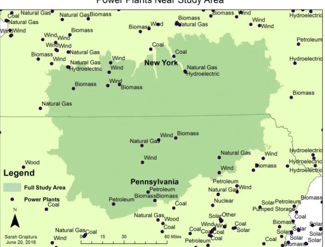
To account for possible fuel switching between various fuel sources, which would obscure air pollution results, the existence of fossil fuel plants within the study area was investigated. Within the study area, there are no coal plants in Pennsylvania; however there is one coal plant on the edge of the study area in northern New York, as shown in Figure 2. In the Pennsylvania study area, there are two natural gas plants, two biomass plants, and one petroleum plant. In the New York study area, there are three natural gas plants and two biomass plants. Future work aims to include controls on fuel switching at various study area plants.

(14)

2.2DATA

To answer the research question, this study mainly combines two types of data: hospital inpatient records and oil and gas well drilling records. The State Inpatient Database (SID) is organized by The Healthcare Cost and Utilization Project (HCUP) and includes all patients, regardless of payer, giving a unique view of inpatient care in a defined market or State over time (HCUP online). Each observation in the dataset represents a patient, and includes more than 70 data elements, including principal and secondary diagnoses and procedures, patient

demographics (sex, age, race, home zip code, etc.), admission and discharge status, length of stay, and payment information. The date of hospitalization is not given to protect patient privacy; however the quarter in which the hospitalization took place is given. An inpatient is defined as a patient who has been formally admitted to the hospital by a doctor, while an outpatient is a patient who is receiving emergency department services, observation services, outpatient surgery, lab tests, X-rays, but has not been formally admitted to the hospital (Medicare online).

Since this study focuses only on Pennsylvania and New York, data was only acquired for these two states. Pennsylvania and New York hospitals are required to report complete inpatient records quarterly to the Pennsylvania Health Care Cost Containment Council (PHC4) and the New York State Department of Health’s Statewide Planning and Research Cooperative System (SPARCS), and in turn this data is incorporated into the SID. Data requests were sent to both PHC4 and SPARCS for their respective inpatient datasets for years 2007-2012. Hospital outpatient and emergency room records were not used in this study because not all New York hospitals are required to report this data to SPARCS. The years 2007-2012 were selected in order to capture time before and during the fracking boom in Pennsylvania. These years were selected by reviewing oil and gas well data.

(15)

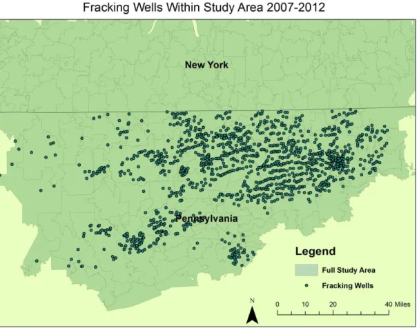
The Pennsylvania Department of Environmental Protection (PDEP) provides statewide oil and gas reports in the form of a GIS shapefile. It includes all oil and gas wells drilled within the state since 1900, and is updated quarterly. The shapefile includes the longitude and latitude of the well, operator, well type (gas, oil, etc.), well status (active, plugged, abandoned, etc.), well pad name, well configuration, date permitted, date drilled, date plugged (if applicable), and if the well is conventional or unconventional. To create the dataset of fracking wells, observations were first limited to fracking wells by selecting those wells that were indicated to be both horizontal and unconventional. This limitation reduced the dataset to 15,478 observations from 159,196. Next, the dataset was limited to only those Pennsylvania counties of interest, by using the clip geoprocessing function in ArcGIS, limiting the dataset to 8,864 observations. Of these wells, 4,271 had no “spud date”, or date the well was drilled, because these wells were only permitted, but not drilled. Therefore these 4,271 observations were removed from the dataset, leaving 4,593 observations. This is not cause for concern because these wells were simply included in the dataset because the wells were only permitted but not drilled. The dataset was then narrowed to the study time period, Quarter 1 of 2007 through Quarter 4 of 2012 (January 1, 2007 through December 31, 2012), by selecting those wells with a spud date before December 31, 2012, thus limiting the dataset to 3,236 observations. Of these wells, one well was removed because its spud date was invalid, leaving the total number of wells to 3,235. A spatial join in ArcGIS was then used to assign zip codes to the wells of interest, based on their location. Figure 5 demonstrates the fracking wells within the study area.

The years 2007-2012 were selected to provide a pre-treatment period where no wells were drilled while also capturing the most intensive fracking years within the study area. Within the study area, the first fracking well was drilled in Quarter 3 of 2007, seven in Quarter 1 of

(16)

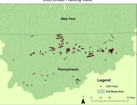
2008, accelerating through Quarter 4 of 2011 with 352 fracking wells drilled in that quarter. Figures 6 to 8 demonstrate the spatial distribution of wells from 2007 to 2012. Figures 24 to 31 demonstrate the number of active wells in Pennsylvania every three quarters for the entire study period.

Population data was gathered for years 2007-2012. Zip code level population counts or estimates were not available for years 2007, 2008, and 2009, so yearly estimates were

extrapolated using the U.S. Census’ Profile of General Demographic Characteristics: 2000 and 2010. For the years 2011 and 2012, the American Community Service’s ACS Demographic and Housing Estimates were used. Quarterly zip code population data was unavailable; hence yearly population values were used. The U.S. Energy Information Administration (EIA) provides data in the form of shapefiles regarding information on shale plays in the United States.. The Shale Gas and Oil Plays, Lower 48 States shapefile was used to determine the location of the Marcellus and Utica shale plays in New York and Pennsylvania. Zip code, county, state, country polygons comes from the TIGER/Line Shapefiles Data Catalog, through the U.S. Census Bureau.

The hospital admission data and well data was combined to create a balanced panel dataset with the unit of observation being a zip code within the study area at a given quarter in time, 2007-2012, quarters 1 to 24. The inpatient data includes the patient’s home zip code, regardless of the location of the hospital at which they were treated. Using this zip code

information, the quarter in which the patient was admitted, and the population of that zip code in a given quarter, per capita admission rates were calculated for each zip code per quarter by dividing the number of patients admitted per quarter by the total zip code population.

Furthermore, the patient age was used to find the number of patients admitted for age groups 0 to 9, 10 to 19, 20 to 64, and 65 and over. These values were then divided by the zip code

(17)

populations of the age group of interest, creating age-specific per capita respiratory admission rates. This health information was then joined by zip code and quarter to the fracking well data, creating the full panel.

The full study region was comprised 297 zip codes, specifically 173 New York zip codes and 124 Pennsylvania zip codes, as shown in Figure 3. To account for air pollution spillovers from Pennsylvania to New York, a buffer region were constructed along the state border and excluded from the analysis. This was achieved in GIS by creating a 5 mile buffer on either side of the border (10 miles total) and excluding zip codes whose centroid fell within this buffer region. This study area and the eliminated zip codes are shown in Figure 4. This process resulted in the exclusion of 43 zip codes, leaving 254 total zip codes, 150 New York and 104

Pennsylvania.

2.3EMPIRICAL STRATEGY

To answer the research question, I examine inpatient respiratory hospitalization rates against varying intensities of drilling in the Marcellus and Utica shale plays of Pennsylvania, with my outcome being the number of per capita respiratory- related hospital admissions within a given zip code at a given time. As a counterfactual, I will use zip codes within bordering New York counties that did not experience any fracking due to the New York State fracking

moratorium that started in July 2008 and resulted in the eventual December 2014 ban. There was no unconventional shale development in New York State before the implementation of the moratorium. This area was chosen as a counterfactual because of the absence of fracking, and because it has similar shale potential and is geologically similar to the treatment counties in Pennsylvania. If counties within Pennsylvania lacking fracking potential were used as the

(18)

counterfactual, one might worry that these counties were inherently different than those counties with intensifying fracking operations. The two Pennsylvania and New York study regions are also rural in character.

To account for movement of air pollution across the New York-Pennsylvania border, I will create a band of excluded zip codes, where I eliminate zip codes within 5 miles on either side of the border. There is not clear consensus within the literature about how far air pollution from hydraulic fracking travels. As Meng (2014) points out, recent studies have failed to feature any rigorous spatial analyses that definitively link various health and environmental risks to distances from fracking sites. Coons (2008) and McKenzie et al. (2012) show that the highest air emissions exist within 0.8 km of an active well. However, birth effects of mothers living near fracking wells are seen as far as 3.5 km from an active well (Hill 2013). Osborn (2011) found methane concentrations in drinking water wells in northeastern Pennsylvania increase, reaching potentially explosive levels, as the distance the active gas-extraction areas decrease. Similarly, Jackson et al. (2013) measured pollutant levels in Marcellus drinking water wells and found methane concentrations to be six times higher and ethane concentrations to be 23 times higher for homes less than 1 km from fracking wells, likely due to stray gas. In Meng’s (2015) distance-based risk analysis model of hydraulic fracking in Pennsylvania, he creates group risk levels of high (<1 km), moderate (1-2 km), and low (2-3 km) risks, and assumes there is little impact beyond 3 km on the environment and inhabitants. Since this study consists of a zip code level analysis, when distances of 1-3 km were used, no zip code centroids fell within this small distance. Therefore, a distance of 5 miles on either side of the border was used as the bandwidth to eliminate zip codes around the border, as shown in Figure 4.

(19)

From 2006 onward, fracking has intensified in Pennsylvania. Within the study area, the first horizontal unconventional well was drilled on May 20, 2007, with no other wells being drilled in 2007. The number of additional active horizontal unconventional wells then

accelerates: 38 more in 2008, 367 more in 2009, 840 more in 2010, and 1,231 more in 2011. This acceleration can be seen for selected zip codes in Figures 17-23 and in Figures 24-31 for active well snapshots for every third quarter. The time frame for this study will be 2007 to 2012, which each time interval being an interval of three months. The timing of the treatment in each zip code will depend on when individual wells were drilled within zip codes; hence, the pre-treatment and treatment period will differ for each zip code, and vary in intensity within each time period. The full model takes the form:

(1) 𝐴𝑑𝑚_𝑧𝑡 = 𝛽₀+ 𝛽₁𝑋_𝑧𝑡1:5_{+ 𝛽}

2𝑋𝑧𝑡6:10+ 𝛽3𝑋𝑧𝑡11:15+ 𝛽4𝑋𝑧𝑡16++ 𝛿𝑧+𝛾𝑡+ 𝜃2007−2012+ 𝜀𝑧𝑡

where 𝐴𝑑𝑚_𝑧𝑡 is the number of per-capita hospitalizations with the primary ICD-9 code classified as a respiratory ailment. The subscript z denotes a given New York or Pennsylvania zip code and the subscript t denotes a given three-month time interval, or quarter from January

2007-December 2012. The superscript on the 𝑋_𝑧𝑡 variables represents the number of active unconventional horizontal wells within a zip code at a given time. Incorporating these

dimensions, X is a treatment dummy variable that takes the value 1 depending on the number of active wells within a specific zip code and quarter. For example, if there are five active wells within a zip code in a given quarter, 𝑋_𝑧𝑡1:5 would take a value of one, and all other treatment variables would take a value of zero. The 𝛿𝑧 represents zip code level fixed effects for all zip codes included in the regression. Quarterly, or seasonal fixed effects are represented by 𝛾_𝑡 and

(20)

are present for all quarters 1 through 24. Yearly fixed effects are represented by 𝜃_2007−2012 and are present for years 2007-2012. The error term is represented by 𝜀𝑧𝑡.

Based on the increased air pollution near fracking wells as demonstrated by Rabinowitz (2015), Hill (2013)’s conclusion that averse birth effects near fracking wells were likely due to air pollution and not water pollution, and the averse respiratory effects that the same airborne chemicals in fracking pollution are known to cause, it is believed that increasing numbers of fracking wells will increase respiratory ailments in nearby populations. Increased respiratory ailments will be indicated by increased respiratory hospital admission rates. In the model, this will be demonstrated by increasing coefficients for the bins containing more fracking well bins. It is estimated that the well bin coefficients will increase from the full study area to the 5 mile buffer area. This is because air pollution spillovers will be taken accounted for most robustly in the 5 mile buffer area.

(21)

3. RESULTS AND DISCUSSION 3.1SUMMARY STATISTICS

The total study area was composed of 297 zip codes, 173 in New York and 124 in Pennsylvania, as shown in Figure 3. There were 3,225 drilled fracking wells located in the Pennsylvania portion of the full study area, with an average of about 8 active fracking wells per quarter, with a range from 0 to 225 wells being drilled in a quarter. Figures 6 to 8 demonstrate average trends in total active wells within Pennsylvania. The 5 mile buffer study area consisted of 254 zip codes, 150 in New York and 104 in Pennsylvania. There were 3,015 drilled fracking wells in the Pennsylvania portion of the 5 mile buffer study area, with an average of 9.164263 active fracking wells per quarter, with a range of 0 to 225 active wells per quarter.

Once the New York SPARCS data was reduced to only respiratory admissions, it consisted of 49,358 patient observations for years 2007-2012, as shown in Table 1. In the full study area, on average 14 people were admitted to the hospital for respiratory

problems each quarter per zip code, the majority being elderly people. Average admissions data is in Table 3. The mean per capita admission rate in the New York full study area was 0.002362 for ages 0 to 9, 0.000359 for ages 10 to 19, 0.009304 for ages 20 to 64, and 0.009956 for those age 65 and older. These statistics along with the 5 mile buffer area statistics can be seen in Table 4 of the Appendix.

The Pennsylvania PHC4 data consisted of 25,905 respiratory observations for the same time period, as can be seen in Table 1. On average, about 10.5 people per quarter were admitted to the hospital for respiratory ailments, mostly elderly people, as shown in Table 3. The mean per capita admission rate in the Pennsylvania full study area was

(22)

0.001719 for ages 0 to 9, 0.000315 for ages 10 to 19, 0.001859 for ages 20 to 64, and 0.012334 for ages 65 and older, as shown in Table 4.

3.2REGRESSION RESULTS

Per-capita respiratory hospital admissions were estimated for three different study areas. The first study area comprised the entire study area, with no border zip codes being excluded. The second study area excluded zip codes on either side of the border whose centroid fell within five miles of the Pennsylvania-New York border. The third study area excluded zip codes on either side of the border whose centroid fell within ten miles of the Pennsylvania-New York border. In addition to these three areas, regressions were also run for separate age groups, specifically ages 0 to 9, 10 to 19, 20 to 64, and 65 and over. These age groups were chosen to represent the very young, teenagers, adults, and elderly.

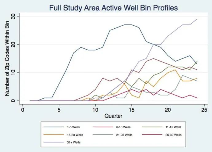
Using the specification described in Equation 1 to measure the effect of varying levels of shale development on respiratory health admissions, the active wells were grouped into bins, specifically 1-5 wells, 6-10 wells, 11-15 wells, 16-20 wells, 21-25 wells, 26-30 wells, and 31 or more wells. The number of zip codes that fall in each bin can be seen in Figure 9. Several other bin schemes were experimented with, and all showed similar results; however, only one bin scheme is reported in this paper. Regression results from a second bin scheme can be viewed in the Appendix.

(2) 𝐴𝑑𝑚𝑧𝑡 = 𝛽0+ 𝛽1𝐴𝑐𝑡𝑖𝑣𝑒𝑊𝑒𝑙𝑙𝑠𝑧𝑡1−5+ 𝛽2𝐴𝑐𝑡𝑖𝑣𝑒𝑊𝑒𝑙𝑙𝑠𝑧𝑡6−10+ 𝛽3𝐴𝑐𝑡𝑖𝑣𝑒𝑊𝑒𝑙𝑙𝑠𝑧𝑡11−15

+ 𝛽3𝐴𝑐𝑡𝑖𝑣𝑒𝑊𝑒𝑙𝑙𝑠𝑧𝑡16−20+ 𝛽3𝐴𝑐𝑡𝑖𝑣𝑒𝑊𝑒𝑙𝑙𝑠𝑧𝑡21−25+ 𝛽3𝐴𝑐𝑡𝑖𝑣𝑒𝑊𝑒𝑙𝑙𝑠𝑧𝑡26−30

+ 𝛽₃𝐴𝑐𝑡𝑖𝑣𝑒𝑊𝑒𝑙𝑙𝑠_𝑧𝑡31+_{+ 𝛿}

(23)

This regression was run for the two different study areas and various age groups. For the full study group, the results showed statistically significant results for the 65 and over population, as shown in Table 5. All reported coefficients are relative to a zip code that has no wells. In

particular, having 1 to 5 active wells in a zip code increased elderly admissions by 0.00347. In comparison to the age 65 and older mean admission rate of 0.011853, this is about a 29% increase in admissions. By multiplying this coefficient by the average 65+ population for Pennsylvania zip codes, we find this coefficient translates to about an additional 1.7 elderly patients per zip code per quarter. For the entire study period, this equals about an additional 644 elderly people admitted to the hospital. This estimate was found by multiplying the number of zip code-quarters that fell into this 1-5 bin by the quarterly zip code increase of 1.717. These calculations can be seen in Table 9, and are used to calculate the number of additional patients in the remainder of the Results section. Having 21 to 25 active wells increased elderly admissions by 0.00268, or about a 23% increase from the mean admission rate of 0.011853. This equals about an extra 1.3 people per zip code each quarter, or about an additional 70 elderly people during the entire study period. Lastly, having 26 to 30 wells increased elderly admissions by 0.00191, or about a 16% increase in the admission rate. This is equal to an additional 1 person per zip code each quarter and about an additional 30 elderly admissions for the entire study period. Overall, the results show a total of about 744 additional elderly patients were admitted for the entire study period 2007-2012. The results also showed that for the age 10 to 19 group, admissions decreased by 0.000205, or a decrease of about 68% from the average age 10 to 19 admission rate. This equals 0.079 less inpatients each quarter, or about 4 less patients for the

(24)

entire study period. This was not significant in the other two study area regressions. The results showed nothing else to be statistically significant.

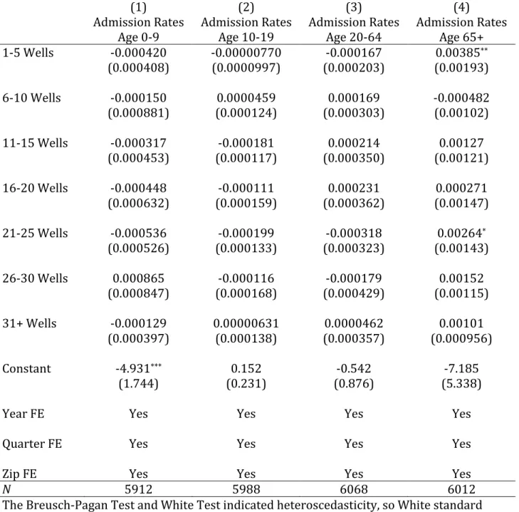
The same regression was run for the 5 mile exclusion area, as shown in Table 6. The results were very similar to the full study area results, but the elderly 26-30 well bin was no longer significant, and the 21-25 well bin for ages 10 to 19 was no longer significant. The coefficient on the 1-5 well bins for the elderly age group became slightly larger in this

regression, increasing to 0.00385, or about a 31% increase in admissions. This translates to about an additional 2 additional elderly patients per zip code per quarter, or a total of about 623

additional elderly patients for the whole study period. The 21-25 bin coefficient slightly decreased to 0.00264, or about a 21% increase in admissions. This corresponds to about an additional 1.3 additional elderly patients per zip code each quarter, or a total of about 65 additional elderly patients for the entire study period, bringing the total to about an additional 689 elderly patients for the entire study period. The results showed nothing else to be significant, as shown in Table 6.

(25)

4. CONCLUSIONS AND LIMITATIONS

The results varied across bins, study areas, and age groups. The number of active wells was found to be significant when the active wells were organized into bins. Of all the bins, only the well bins for the age 65 and older group were significant, across both study areas. The only exception to this was in the full study area, the 21-25 well bin was significant for the age 10-19 group; however this was not significant for the 5 mile buffer area. This could be an indication of the 5 mile buffer study area correcting for spillovers. There were no statistically significant results for any other age group, or for any other bin, across both study areas. When other bin schemes where experimented with, typically only the bin with the smallest number of wells was significant.

The significance of only certain bins, typically the bin with the smallest number of wells does not support the hypothesis that more active wells would lead to higher respiratory

admission rates through the mechanism of increased air pollution. For this hypothesis to be supported, all fracking well bins would have had statistically significant coefficients, with the bins with larger amounts of wells having larger positive coefficients. However, it still indicates that active fracking wells do affect elderly respiratory hospital admissions.

One explanation for the smallest bin being statistically significant could be the fact that inpatient, and not outpatient data was used in this analysis. Outpatient data includes emergency room visits, while inpatient data only includes patients that were admitted to the hospital and classified as inpatient, through the emergency room or otherwise. It is possible that patients residing in high-bin zip codes could indeed be visiting the hospital, but are visiting the emergency room and are not being admitted to the hospital as inpatients. In this case, this analysis would not capture these hospital visits, and severely underestimate the effect of active

(26)

wells on high-bin zip code respiratory health. One reason why people in high-bin zip codes could frequent the emergency room and bypass being admitted as an inpatient more than those people living in low-bin zip codes could be that perhaps those patients were already admitted for respiratory problems early on in their zip code undergoing shale development, or when their zip code would be considered a low-bin zip code. Potentially, they would be less likely to be admitted as an inpatient again, and would likely just visit their doctor’s office or emergency room directly if they kept having continued respiratory problems, since these patients were likely prescribed respiratory treatments such as nebulizers, etc. which would render further hospital admissions unnecessary. Since emergency room data and doctor’s office data was not available for both Pennsylvania and New York, this hypothesis cannot be tested without further research. Nonetheless, this study serves as a lower-bound estimate for the effect of shale gas development on respiratory health. A study repeating this procedure with outpatient data has the potential to find an upper bound and possibly give a better explanation of what is happening in the high-bin zip codes.

Another explanation for these results could be that elderly people die before they become inpatients during high shale development, or when zip codes fall into the larger bins. In this case, patients would not be counted as respiratory inpatients. This would decrease the respiratory admission rates in counties of high shale gas development.

Furthermore, it is possible that people who reside in fracking zip codes could be

exhibiting averting behavior. Examples of such averting behavior include elderly people going on less walks outside, less summer sunbathing, closing more windows, or less cooking outdoors due to unpleasant smells or noises. This phenomenon could be affecting the regression results, causing the lowest bin to typically be significant, while higher bins are not significant. In a

(27)

February 2011 New York Times video, residents of Garfield County, Colorado report foul smelling fumes and odors from nearby condensate storage tanks that caused them to stay inside, and eventually move from their home altogether.

Another issue that will be addressed in future research is the potential of fuel switching and production trends of the power plants within and near the full study area. Local demand or fuel switching could possibly confound air pollution results.

To conclude, the results suggest that fracking wells increase respiratory hospital

admissions for people age 65 and older by 16 -31%, but there is no significant evidence showing that admission rates were increased for any other age group. Regression results typically have the same sign, but smaller magnitude when comparing the 5 mile buffer area to the full study area regressions. Further research should address the potential pitfalls discussed, including averting behavior in those people living near fracking wells, the deaths of elderly people near fracking wells, the distance that fracking air pollution travels, and the difference between emergency room visits and hospital admissions, possibly in a different location where emergency records are available.

(28)

5. REFERENCES

Armenderiz, E., & Fund, E. D. (2009). Emissions from natural gas production in the Barnett shale area and opportunities for cost-effective improvements.

Bamberger, M., & Oswald, R. (2012). Impacts of gas drilling on human and animal health. NEW SOLUTIONS: A Journal of Environmental and Occupational Health Policy, 51-77.

Boslett, Andrew, Todd Guilfoos, Corey Lang. 2015. “Valuation of Expectations: A Hedonic Study of Shale Gas Development and New York’s Moratorium.”

Boxall, Peter C, Wing H. Chan, Melville M. McMillan. 2005. “The impact of oil and natural gas facilities on rural residential property values.” Resource and Energy Economics 27 248-269. Cascio, Elizabeth U. and Ayushi Narayan. 2015. “Who Needs a Fracking Education? The

Education Response to Low-Skill Biased Technological Change.” NBER Working Paper number 21359.

Chapman EC, Capo RC, Stewart BW, Kirby CS, Hammack RW, Schroeder KT, et al. 2012. Geochemical and strontium isotope characterization of produced waters from Marcellus Shale natural gas extraction. Environ Sci Technol 46:3545–3553.

Colborn, T., Kwiatkowski, C., Schultz, K., & Bachran, M. (2011). Natural gas operations from a public health perspective. Human and Ecological Risk Assessment: An International Journal, 17(5), 1039-1056.

Colborn, T., Schultz, K., Herrick, L., & Kwiatkowski, C. (2012). An exploratory study of air quality near natural gas operations. Human and Ecological Risk Assessment: An International Journal.

Coons, Teresa, and Russell Walker. "Community health risk analysis of oil and gas industry impacts in Garfield County." Grand Junction: Saccomanno Research Institute (2008). Cosgrove, Brandan. 2014. “The Economic Impact of Shale Gas Development: A Natural Experiment along the New York and Pennsylvania Border.” Colby College Digital Commons Honors Theses.

DeLeire, Thomas, Paul Eliason, Christopher Timmins. 2014. “Measuring the Employment Impacts of Shale Gas Development.” Working Paper.

Gilman, J., Lerner, B., Kuster, W., & de Gouw, J. (2013). Source signature of volatile organic compounds from oil and natural gas operations in northeastern Colorado. Environmental Science and Technology, 47(3):1297-1305.

Goetz, J.D., C.R. Floerchinger, E. Fortner, J. Wormhoudt, P. Massoli, S. Herndon, C.E. Gopalakrishnan, S., & Klaiber, H. A. (2014). Is the shale energy boom a bust for nearby residents? Evidence from housing values in Pennsylvania. American Journal of Agricultural

(29)

Economics, 96(1), 43-66.

Gopalkrishan, Sathya, H. Allen Klaiber. 2015. “Is the Shale Boom a Bust for Nearby Residents? Evidence from Housing Values in Pennsylvania.” Working paper.

HCUP online https://www.hcup-us.ahrq.gov/sidoverview.jsp

Howarth, R. W., Santoto, R., & Ingraffea, A. (2011). Methane and the greenhouse-gas footprint of natural gas from shale formations. Climatic Change, 106(4), 679-690.

Jackson, R.B., Vengosh, A., Darrah, T.H., Warner, N.R., Down, A., Poreda, R.J., Osborn, S.G., Zhao, K., Karr, J.D., 2013. Increased stray gas abundance in a subset of drinking water wells near Marcellus shale gas extraction. Proc. Natl. Acad. Sci. U.S.A. 110,11250.

James, Alexander and Brock Smith. 2014. “There Will Be Blood: Crime Rates in Shale-Rich U.S. Counties.” OxCarre Research Paper 140.

Kargbo, D. M., Wilhelm, R.G. & Campbell, D.J. (2010). Natural gas plays in the Marcellus shale: Challenges and potential opportunities. Environmental Science & Technology, 44(15) 5679-5684.

Kolb, B. Knighton, E.M. Knipping, and S.L. Shaw. 2013. “Site Specific Emission of Marcellus Shale Development Using Fast Mobile Measurements.” American Geophysical Union Fall Meeting 2013. Abstract #A44E-04.

Komarek, Timothy. 2015. “Labor Market Dynamics and the Unconventional Natural Gas Boom: Evidence from the Marcellus Region.” Researchgate.

Hill, Elaine L. 2013. “Unconventional Natural Gas Development and Infant Health: Evidence from Pennsylvania.” Working paper.

Kovats S, Depledge M, Haines A, Fleming LE, Wilkinson P, Shonkoff SB, et al. 2014. The health implications of fracking. Lancet 383:757–758.

LaRiviere, Jacob, Joseph Shapiro, Nathan Tefft, Hendrik Wolff. 2014. “Quantifying Environmental Benefits of Fracking: The Decline of Coal, Air Quality and Asthma Rates”. Working Paper, April 2014.

Litovitz, A., Curtright, A., Abramzon, S., Burger, N., & Samaras, C. (2013). Estimation of regional air-quality damages from Marcellus shale natural gas extraction in Pennsylvania. Environmental Research Letters, 8(1), 014017.

"Marcellus, Utica Provide 85% of U.S. Shale Gas Production Growth since Start of 2012." U.S. Energy Information Administration - EIA - Independent Statistics and Analysis: Today in Energy. U.S. Energy Information Administration, 28 July 2015. Web. 2016.

(30)

Development.

Medicare online https://www.medicare.gov/Pubs/pdf/11435.pdf

McKenzie LM, Guo R, Witter RZ, Savitz DA, Newman LS, Adgate JL. 2014. Birth outcomes and maternal residential proximity to natural gas development in rural Colorado. Environ. Health Perspect.

McKenzie L., Witter R., Newman L., & Adgate J. (2012) Human health risk assessment of air emissions from development of unconventional natural gas resources. Science of The Total Environment.

Meng, Q., Ashby, S. 2014. Distance: A critical aspect for environmental impact assessment of hydraulic fracking. The Extractive Industries and Society 1(2014) 124-126.

Meng, Q. (2015). Spatial analysis of environment and population at risk of natural gas fracking in the state of Pennsylvania, USA. Science of The Total Environment, 515, 198-206.

Muehlenbachs, Lucija Anna, and Alan J. Krupnick. "Shale Gas Development Linked to Traffic Accidents in Pennsylvania." Blog Post. Resources for the Future, 27 Sept. 2013. Web. 2 Dec. 2015.

Muehlenbachs, Lucija, Elisheba Spiller, Christopher Timmins. 2012. “Shale Gas Development and Property Values: Differences Across Drinking Water Sources.” NBER Working Paper 18390.

Muehlenbachs, Lucija, Elisheba Spiller, Christopher Timmins. 2013 “The Housing Market Impacts of Shale Gas Development.” RFF DP 13-39.

Northrup JM, Wittemyer G. 2013. Characterising the impacts of emerging energy development on wildlife, with an eye towards mitigation. Ecol. Lett. 15(1):112-125.

Olsen, Erik. “Natural Gas and Polluted Air.” New York Times. February 26, 2011. http://www.nytimes.com/video/us/100000000650773/natgas.html

Osborn, S. G., Vengosh, A., Warner, N. R., & Jackson, R. B. (2011). Methane contamination of drinking water accompanying gas-well drilling and hydraulic fracturing. proceedings of the National Academy of Sciences,108(20), 8172-8176.

Paredes, Dusan, Timothy Komarek, Scott Loveridge. 2015. “Income and employment effects of shale gas extraction windfalls: Evidence from the Marcellus region.” Energy Policy 47 (112-120).

Parker, Dominic, and Daniel Phaneuf. 2013. “The Potential Impacts of Frac Sand Transport and Mining on Tourism and Property Values in Lake Pepin Communities.”

(31)

Pétron, G., Frost, G., Miller, B.R., Hirsch, A.I., Montzka, S. A., Karion, A.,…others (2012). Hydrocarbon emissions characterization in the Colorado front range: A pilot study. Journal of Geophysical Research: Atmospheres (1984-2012), 117(D4).

Popkin, Jennifer H., Joshua M. Duke, Allison M. Borchers, Thomas Ilvento. 2013. “Social Costs from Proximity to Hydraulic Fracturing in New York State.” Energy Policy 62 62-69.

Rabinowitz PM, Slizovskiy IB, Lamers V, Trufan SJ, Holford TR, Dziura JD,

Peduzzi PN, Kane MJ, Reif JS, Weiss TR, Stowe MH. 2015. Proximity to natural gas wells and reported health status: results of a household survey in Washington County, Pennsylvania. Environmental Health Perspectives, 123:21–26.

Rich, Alisa, James P. Grover, and Melanie L. Sattler. 2014. “An Exploratory Study of Air Emissions Associated with Shale Gas Development and Production in the Barnett Shale.” Journal of the Air & Waste Management Association, 64 (1):61-72.

Rozell DJ, Reaven SJ. 2012. Water pollution risk associated with natural gas extraction from the Marcellus Shale. Risk Anal 32:1382–1393.

Schmidt, C.W. (2011). Blind rush? Shale gas boom proceeds amid human health questions. Environmental Health Perspectives, 119(8).

"Shale in the Unites States." U.S. Energy Information Administration - EIA - Independent Statistics and Analysis. 18 Nov. 2015. Web. 8 Dec. 2015.

Throupe, Ron, Robert A. Simons, Xue Mao. 2013. “A Review of Hydro ‘Fracking’ and its Potential Effects on Real Estate.” Journal of Real Estate Literature. 2013.

U.S. EPA. Assessment of the Potential Impacts of Hydraulic Fracturing for Oil and Gas on Drinking Water Resources (External Review Draft). U.S. Environmental Protection Agency, Washington, DC, EPA/600/R-15/047, 2015.

(32)

APPENDIX

Table 1: Respiratory Admissions Observations Observations

Year Pennsylvania New York

2007 4,232 7,883 2008 4,642 8,615 2009 4,397 8,759 2010 4,121 8,176 2011 4,373 8,279 2012 4,140 7,646

(33)

Table 2: Fracking Well Summary Statistics

Full Study 5 Mile Buffer

Drilled Wells 3,225 3,015

Mean Active Wells 8.19086 9.164263 S.D. Active Wells 23.67132 25.45698

Minimum Active Wells 0 0

(34)

Table 3: Average Quarterly Respiratory Admissions by Age Group (Number of Inpatients)

Age Pennsylvania New York

0-9 Years 0.59039 1.14451 10-19 Years 0.13743 0.21291 20-64 Years 2.75874 3.76806 65+ Years 9.08850 6.76228

(35)

(36)

Table 5: The Effect of Increasing Well Bins on Respiratory Hospital Admissions (Full Study Area)

(1) (2) (3) (4)

Admission Rates

Age 0-9 Admission Rates Age 10-19 Admission Rates Age 20-64 Admission Rates Age 65+ 1-5 Wells -0.000251 -0.0000126 -0.000102 0.00347** (0.000295) (0.0000859) (0.000176) (0.00165) 6-10 Wells 0.000219 0.0000217 0.000320 -0.000644 (0.000720) (0.000105) (0.000264) (0.000891) 11-15 Wells 0.0000337 -0.0000841 0.000252 0.00156 (0.000375) (0.000104) (0.000299) (0.00105) 16-20 Wells -0.000147 -0.0000400 0.000327 0.000490 (0.000573) (0.000148) (0.000313) (0.00133) 21-25 Wells -0.000101 -0.000205* _-0.000177 _0.00268** (0.000404) (0.000119) (0.000280) (0.00132) 26-30 Wells 0.000799 -0.000134 0.0000636 0.00191* (0.000652) (0.000134) (0.000354) (0.000993) 31+ Wells 0.000343 0.00000484 0.000242 0.00134 (0.000383) (0.000123) (0.000300) (0.000867) Constant -4.446 0.593 -1.599 -11.82** (2.863) (0.453) (0.998) (5.649)

Year FE Yes Yes Yes Yes

Quarter FE Yes Yes Yes Yes

Zip FE Yes Yes Yes Yes

N 7128 7128 7128 7128

The Breusch-Pagan Test and White Test indicated heteroscedasticity, so White standard errors were used, and are shown in parentheses

(37)

Table 6: The Effect of Increasing Well Bins on Respiratory Hospital Admissions (5 mile buffer)

(1) (2) (3) (4)

Admission Rates

Age 0-9 Admission Rates Age 10-19 Admission Rates Age 20-64 Admission Rates Age 65+ 1-5 Wells -0.000420 -0.00000770 -0.000167 0.00385** (0.000408) (0.0000997) (0.000203) (0.00193) 6-10 Wells -0.000150 0.0000459 0.000169 -0.000482 (0.000881) (0.000124) (0.000303) (0.00102) 11-15 Wells -0.000317 -0.000181 0.000214 0.00127 (0.000453) (0.000117) (0.000350) (0.00121) 16-20 Wells -0.000448 -0.000111 0.000231 0.000271 (0.000632) (0.000159) (0.000362) (0.00147) 21-25 Wells -0.000536 -0.000199 -0.000318 0.00264* (0.000526) (0.000133) (0.000323) (0.00143) 26-30 Wells 0.000865 -0.000116 -0.000179 0.00152 (0.000847) (0.000168) (0.000429) (0.00115) 31+ Wells -0.000129 0.00000631 0.0000462 0.00101 (0.000397) (0.000138) (0.000357) (0.000956) Constant -4.931*** _0.152 _-0.542 _-7.185 (1.744) (0.231) (0.876) (5.338)

N 5912 5988 6068 6012

The Breusch-Pagan Test and White Test indicated heteroscedasticity, so White standard errors were used, and are shown in parentheses

(38)

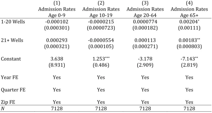
Table 7: The Effect of Increasing Well Bins on Respiratory Admissions (Scheme #2 Full Study Area)

(1) (2) (3) (4)

Admission Rates

Age 0-9 Admission Rates Age 10-19 Admission Rates Age 20-64 Admission Rates Age 65+ 1-20 Wells -0.000102 -0.0000215 0.0000774 0.00204* (0.000301) (0.0000723) (0.000182) (0.00111) 21+ Wells 0.000293 -0.0000554 0.000113 0.00183** (0.000321) (0.000105) (0.000271) (0.000803) Constant 3.638 1.253*** _-3.178 _-7.143** (8.931) (0.486) (2.909) (2.819)

N 7128 7128 7128 7128

𝐴𝑑𝑚𝑧𝑡 = 𝛽0+ 𝛽1𝐴𝑐𝑡𝑖𝑣𝑒𝑊𝑒𝑙𝑙𝑠𝑧𝑡1−20+ 𝛽2𝐴𝑐𝑡𝑖𝑣𝑒𝑊𝑒𝑙𝑙𝑠𝑧𝑡21++ 𝛿𝑧+𝛾𝑡+ 𝜃2007−2012+ 𝜀𝑧𝑡 The Breusch-Pagan Test and White Test indicated heteroscedasticity, so White standard errors were used, and are shown in parentheses

(39)

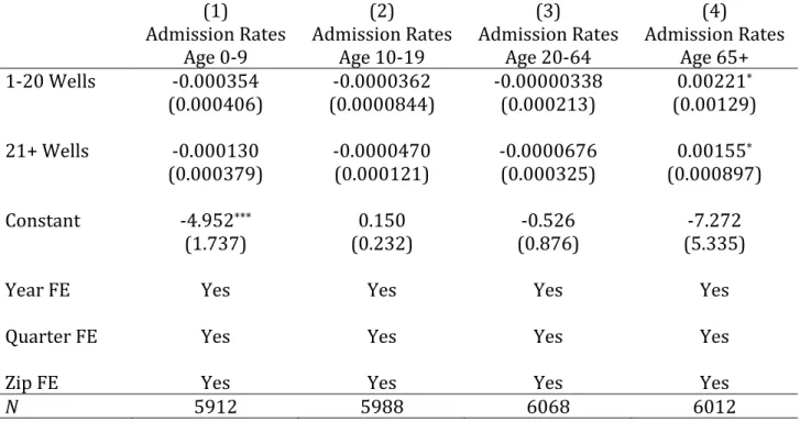
Table 8: The Effect of Increasing Well Bins on Respiratory Hospital Admissions (Scheme #2 5 mile buffer)

(1) (2) (3) (4)

Admission Rates

Age 0-9 Admission Rates Age 10-19 Admission Rates Age 20-64 Admission Rates Age 65+ 1-20 Wells -0.000354 -0.0000362 -0.00000338 0.00221* (0.000406) (0.0000844) (0.000213) (0.00129) 21+ Wells -0.000130 -0.0000470 -0.0000676 0.00155* (0.000379) (0.000121) (0.000325) (0.000897) Constant -4.952*** _0.150 _-0.526 _-7.272 (1.737) (0.232) (0.876) (5.335)

N 5912 5988 6068 6012

𝐴𝑑𝑚𝑧𝑡 = 𝛽0+ 𝛽1𝐴𝑐𝑡𝑖𝑣𝑒𝑊𝑒𝑙𝑙𝑠𝑧𝑡1−20+ 𝛽2𝐴𝑐𝑡𝑖𝑣𝑒𝑊𝑒𝑙𝑙𝑠𝑧𝑡21++ 𝛿𝑧+𝛾𝑡+ 𝜃2007−2012+ 𝜀𝑧𝑡 The Breusch-Pagan Test and White Test indicated heteroscedasticity, so White standard errors were used, and are shown in parentheses

(40)

(41)

(42)

(43)

(44)

(45)

(46)

(47)

(48)

(49)

(50)

(51)

(52)

(53)

(54)

(55)

(56)

(57)

(58)

(59)

(60)

(61)

(62)

(63)

(64)

(65)

(66)

(67)

(68)

(69)

(70)

(71)

Shale gas development and respiratory health

Table of Contents