The Cyclical Dynamics of Investment: The Role of Financing and Irreversibility Constraints

CFCM

C

ENTRE

F

OR

F

INANCE

A

ND

C

REDIT

M

ARKETS

Working Paper 07/10

The Cyclical Dynamics of Investment:

The Role of Financing and Irreversibility

Constraints

John Tsoukalas

Produced By:

Centre for Finance and Credit Markets

School of Economics

Sir Clive Granger Building

University Park

Nottingham

NG7 2RD

Tel: +44(0) 115 951 5619

Fax: +44(0) 115 951 4159

enquiries@cfcm.org.uk

The Cyclical Dynamics of Investment: The Role of

Financing and Irreversibility Constraints

John D. Tsoukalas

School of Economics, University of Nottingham, University Park, Nottingham, NG7 2RD

This draft: January 2007

Abstract

This paper develops a rich decision theoretic dynamic firm model that analyzes pro-ductivity and interest rate shocks. The model is used to analyze the cyclical dynamics of fixed and inventory investment and in particular asks whether constraints to the flow of funds can generate the frequently overlooked fact that investment in input in-ventories leads investment in fixed capital in business cycle frequencies. To account for this regularity the model proposes a combination of irreversibility and financing con-straints. The usefulness of this explanation in relation to competing hypotheses, relies on the fact that it is also consistent with a list of facts from the inventory research. In addition it is shown that under persistent shocks, financing constraints are sufficient but not necessary to explain procyclicality. This implies that fixed investment cash flow regressions may not be informative for the presence of capital market imperfec-tions because positive correlaimperfec-tions can arise even under perfect capital markets. Last, analysis of interest rate shocks implies that the effects on inventory spending are quite small in relation to effects arising from productivity shocks.

JEL classification: D21; E22; E32; G31

Key words: Financing Constraints; Inventories; Investment; Perturbation methods; Time-to-build

This is a revised version of Chapter 2 from my 2003 PhD dissertation at the University of Maryland College Park. I am grateful to John Haltiwanger, Michael Pries, Plutarchos Sakellaris and John Shea for inspiration, encouragement and valuable suggestions. I would also like to thank colleagues from the Bank of England, Spiros Bougheas and Paul Mizen for detailed comments on a later draft, and to seminar participants at the Cardiff Business School.

1

Introduction

It is a well known fact that inventory investment is procyclical. This is one of the two key stylized facts stressed in the survey of inventory research by Ramey and West (1999). Moreover, manu-facturers’ materials and supplies are one of the largest and most volatile components of inventory investment, as documented in many studies. Blinder and Maccini (1991) argue that much of the cyclical fluctuation in manufacturing inventories is due to raw materials and work-in-progress as opposed to finished goods. In motivating their study Humphreys et al. (2001) document that invest-ment in input inventories is more than three times more variable than investinvest-ment in finished good inventories. Further, as documented by the same authors, the cyclical behavior of input inventory investment is a consequence of the volatility and procyclicality of materials deliveries in relation to materials usage. An interesting yet overlooked fact is that investment in input inventories leads investment in fixed capital in both aggregate and manufacturing U.S. data.1 _{Bernanke and Gertler}

(1995) indirectly document this timing difference in their survey of results for the “credit channel” view of the monetary policy transmission mechanism by showing fixed investment lags behind other types of spending following a monetary policy shock. The purpose of this paper is to propose an explanation for this fact while being consistent with a number of facts from the inventory research. Our model has the following three features: a realistic time-to-build assumption in the produc-tion of fixed capital, irreversibility of fixed investment and financing constraints. Clearly one could rationalize the timing difference between investment and other spending by appealing to gestation lags (time-to-build) for fixed capital. The problem with this explanation is two-fold. First, it would require an assumption on the length of the gestation lag for fixed capital that is not supported by the existing empirical evidence.2 _{Second, and more importantly, a pure time-to-build argument}

does not pass the inventory stylized fact list and in particular it fails to generate procyclicality of inventory investment.

The model outlined in this paper can account for the dynamic correlations between investment in fixed capital and inventories while being consistent with the stylized inventory facts as documented in Humphreys et al. (2001) and recently analyzed by Caggese (2007). It is important to stress that the role of financing constraints is very important for the model’s ability to match the empirical dynamic correlations. Intuitively, because investment in fixed capital is irreversible, an adverse productivity shock causes only a limited decline in investment compared to optimal. This implies that fixed capital is higher than the level implied by lower productivity. At the same time, the

1_{Moreover the same fact holds for U.K. data.}

2_{In addition as Bernanke and Gertler (1995) emphasize equipment investment, which will be characterized}

presence of financing constraints implies that internal liquidity is valuable. Given that the level of the capital stock is high compared to the optimal, this incentives the firm to persistently spend less on capital projects in order to economize on liquidity, giving rise to a hump-shaped response of fixed investment. Thus irreversibility of fixed investment is crucial for this result and without it, capital would move in line with productivity and fixed investment would respond more sharply (in order to adjust a slowly depreciating capital stock).

The paper analyzes a rich-decision theoretic model that encompasses both productivity and interest rate shocks. The analysis presented here complements the work of Maccini et al. (2004) on the relationship between variation in interest rates and inventories in the long run by analyzing the dynamics of input inventories in response to real interest rate variation in the short run. This is important because the analysis provides a natural link to the monetary policy transmission mecha-nism question from the perspective of inventory spending. Monetary policy exerts its influence on aggregate demand by controlling a short-term interest rate, therefore the first step in understanding the transmission mechanism is to develop a foundation that allows to study the effects of interest rate changes. The simulations of the model imply that quantitatively the effect of interest rate variation is quite small compared to productivity disturbances. This finding is consistent with the empirical evidence presented in Maccini et al. (2004).

Finally, the paper shows that procyclicality in materials deliveries and fixed investment does not necessarily imply financing constraints. Under persistent shocks and irreversibility of fixed investment procyclicality arises even with perfect capital markets. In the simulations presented un-der irreversibility and perfect capital markets, fixed investment and cash-flow are nearly perfectly correlated. This implies that empirical work that relies on the cash-flow—fixed investment rela-tionship in reduced form regressions are not necessarily informative about the presence of capital market imperfections. This finding is related to Gomez (2001) who shows that reduced form fixed investment equations that include cash-flow as an explanatory variable will be likely mis-specified, and will incorrectly assign a role to cash-flow. Although the reasons in Gomez (2001) are quite different, namely specification and measurement errors, the prediction is the same.

This paper is mostly related to Caggese (2007), which focuses on the procyclicality of materials deliveries and inventory investment and their asymmetric behavior over the business cycle, relying on a similar modelling approach.3 _{This paper provides additional insights by focusing on the aspect}

of timing of fixed and inventory investment, the validity of fixed investment cash flow correlations for the significance of capital market imperfections, and an analysis of interest rate shocks while

3_{Holt (2003) is another paper that examines the implications of both financing and irreversibility}

confirming the findings in the earlier paper.

The rest of the paper is organized as follows. Section 2 describes the model. Section 3 discusses the solution and calibration. In Section 4 results from the simulated version of the model are presented. Section 5 concludes.

2

The Model

The model analyzed incorporates the joint decisions of firms in fixed and inventory investment in the presence of financial constraints. The following subsections explain the components that are essential to the framework.

2.1

Firms

2.1.1 Technology

There is an entrepreneurial sector which is populated by a continuum of risk-neutral infinitely-lived firms. Firmj produces output, using the following decreasing returns to scale Cobb-Douglas tech-nology:4

yt=AtF(Kt, Mt, Lt) =AtKtαMtγLνt γ+α+ν <1

whereA_t is an idiosyncratic productivity shock,K_tis capital, M_tis the stock of materials, and L_t

is the labor input. Following empirical work by Ramey (1989) and more recently Humphreys et al. (2001),Mtcan be thought as input materials and/or work-in-process. Additions to the capital stock

is subject to gestation lags. Specifically, I assume a 2-periodtime-to-build for new capital projects. The time-to-build requirement implies that in any given period t, firms initiate new projects, s2t,

and complete partially finished projects, s1t. This assumption intends to capture the design and

construction stages that exist in undertaking investment projects in plant and equipment. The

time-to-build feature of capital projects is emphasized by Kydland and Prescott (1982). Formally:

s_2t=s_1,t+1 (2.1)

Kt+1 = (1−δ)Kt+s1t (2.2)

It=ϕ1s1t+ϕ2s2t, ϕ1+ϕ2 = 1 (2.3)

4_{Decreasing returns to scale are necessary for firm size to be well defined. Otherwise firm size is}

where s2t denotes new projects at time t, s1t denotes projects initiated at time t−1, δ is the

depreciation rate of the capital stock, andItdenotes total investment expenditures at timet. The

parameters ϕ1 and ϕ2 represent the fraction of resources allocated to projects that are 1 and 2

periods away from completion respectively.5

In addition the firm places materials ordersdt, for use in production in periodt+ 1,Mt+1. The

stock of materials thus evolves according to:

Mt+1 = (1−δm)Mt+dt (2.4)

Note that this timing convention assumes that orders of materials at timetenter the firm after current production has taken place.

Last, firms hire labor from a competitive market at a given (constant) wage rate, w.

2.1.2 Financing

Firms face financing constraints in making their investment—in fixed capital and inventories—and employment decisions. Specifically, the flow of funds into the firm is restricted in the following ways. Firms in this industry are not allowed to issue fresh equity, implying that dividends must be non-negative.

div_t≥0 (2.5)

Firms can borrow to finance expenditures subject to an exogenous limit (BLim_{). The credit}

mar-ket is assumed to extend one-period (secured) debt only. A limited enforceability argument (see Albuquerque and Hopenhayn (1997)) can justify this exogenous limit.

Bt+1(1 +rt+1)6BLim (2.6)

In the calibration exercise I assume that this limit is equal to the value of collateralizable (productive) assets a firm can pledge. This is the sum of un-depreciated capital and materials evaluated at the steady state of the model, (1−δm)M+ (1−δ)K.6 Replacing in (2.6) above gives:

(1−δm)M + (1−δ)K

(1 +rt+1) >Bt+1 (2.7)

Thus effectively the borrowing limit varies with the interest rate, i.e., a higher interest rate is associated with a smaller borrowing capacity.

5_{Note that the technological assumptions on projects do not leave firms the option to abandon projects}

in the second period of the construction.

Moreover in order to rule out any other external sources of funds the following constraints must be satisfied.

dt≥0 (2.8)

s_2t≥0 (2.9)

Note that the last two inequalities imply that firms cannot finance expenditures by either selling materials or their capital stock. In particular the last inequality along with the techno-logical assumption on capital projects above effectively makes investment decisions irreversible. Irreversibility can be motivated by the fact that existing production facilities often have very low resale values. The importance and relevance of irreversibility has been highlighted by Bertola and Caballero (1994) and Caballero et al. (1995). Taken together, these nonnegativity constraints pro-hibit the firm from using any source of funds other than internally generated funds and to a limited extent new borrowing.

2.1.3 The firm’s problem

Timing is as follows. At the beginning of period t, the idiosyncratic productivity shockA_t, and r_t

are realized. The firm inherits a stock of capitalKt, materialsMt, half-completed projects s1t, and

debtBt, from the previous period. Then, beforeAt+1 and rt+1 are observed, the firm decides how

to allocate internal funds (cash flow) at time t, and new borrowing,Bt+1, to finance the wage bill,

expenditure on new and existing projects s2t, s1t, materials orders, dt, dividends, divt, and repay

previously accumulated debt,Bt, in order to maximize firm value.

max Lt,s2t,dt,Bt+1 E0 ∞ X t=0  tY−1 j=0 βj  _{divt (2.10)} subject to (2.1),(2.2),(2.4),(2.5),(2.7)-(2.9),7 lnAt+1 =ρAlnAt+σAεt+1 εt∼N(0,1) lnrt+1= (1−ρr)lnr+ρrlnrt+σrυt+1 υt∼N(0,1)

Note that by the equality of sources and uses of funds, dividends are:

7_β

divt=AtKtαMtγLνt −wLt−dt−ϕ1s1t−ϕ2s2t+Bt+1−(1 +rt)Bt (2.11)

From equation (2.11) above one can see that the firm finances expenditures, distributes divi-dends and pays off existing debt either via new debt,Bt+1 or cash flow defined as:

(AtKtαMtγ(Loptt )ν −rtBt) (2.12)

The firm’s problem defined above can be described in six state variables (K, M, s1, B, A, r).

An additional complexity is the presence of both equality and inequality constraints. While the presence of inequality constraints alone do not pose a problem for obtaining a solution based on a global approach (e.g. policy or value function iteration), the fact of the high dimensionality (six state variables) renders such solution methods infeasible for a reasonably accurate characterization of the solution (curse of dimensionality). To circumvent this difficulty a second order perturbation method is used and adapted to permit the accommodation of the inequality constraints in a modified objective function. This way the problem is recast into one with equality constraints and the approximate solution is found using a second order Taylor expansion of the equilibrium conditions. More specifically, the original problem is modified by parametrically incorporating the inequality constraints into the objective function. This is accomplished by modifying the objective function with penalty terms that become larger as the respective constraint approaches its limit.8 _Define pi, i= 1,2,3,4 as the parameter that controls the tightness of constraint i. The period objective

at timet is modified to incorporate the inequality constraints as:

div_t+p₁[divlog(div_t)−div_t]+

p2[s2log(s2t)−s2t] +p3[( B

Lim

(1 +r) −B)log(

BLim

(1 +rt+1) −Bt+1) +Bt+1] +p4[dlog(dt)−dt]

where a bar over a variable denotes its steady state value. For example, the inequality constraint on dividends is accounted for by the termp1[divlog(divt)−divt]. Using this formulation the firm

incurs an increasing penalty as dividends are reduced and approach the no issuance constraint. In the limit as div_t → 0 this term diverges to −∞. The parameter p₁ controls the weight on the penalty. Hence, the functional form of these terms implies that choices approaching the limit of the constraint will hardly be chosen.9 _{The specific way these terms enter the period t dividend}

ensures that the non-stochastic steady state is independent of the parameters pi. In other words

the steady state of this model corresponds to a frictionless (perfect capital markets) equilibrium.

8_{This is an example of the logarithmic barrier method for constrained optimization problems. See Boyd}

and Vandenberghe (2004) for details of this approach.

The Langrangean for the modified problem is max Lt,s2t,dt,Bt+1 E0 ½_X∞ t=0  tY−1 j=0 βj 

_{{divt+p1[divlog(divt)−divt] +p2[s2log(s2t)−s2t]+}

p3[( B Lim (1 +r) −B)log( BLim (1 +rt+1) −Bt+1) +Bt+1] +p4[dlog(dt)−dt]+ λt(Kt+1−(1−δ)Kt−s2t−1) +µt(Mt+1−(1−δm)Mt−dt)} ¾ (2.13) where λt, µt denote the Kuhn-Tucker multipliers associated with the equality constraints. The

first order necessary conditions for this problem are given in the Appendix.

3

Solution

The solution of the model is characterized by a set of Euler equations along with the Kuhn-Tucker conditions for the equality constraints and the given initial values for the state variables. An approximate solution is calculated by using a second order perturbation method around the non-stochastic steady state of the model. The second order Taylor approximation, as described in Schmitt-Grohe and Uribe (2004), is adapted to accommodate the inequality constraints as explained in section 2.1.3 above.10

Perturbation methods, in contrast to global methods such as value/policy function iteration, can easily handle high dimensional state problems like the one described in this paper. The innovation is to tackle the inequality constraints within this approach, and recently some progress has been made on that front (see Kim et al. (2005) that analyze a consumption-asset allocation problem using a similar approach).

3.1

Calibration

In order to analyze the equilibrium of the model and gain intuition on the dynamics the equilibrium conditions of the model are simulated using a baseline set of parameter values as in Table 1. These are discussed below.

The value for the output share of materials, γ, and labor, ν is taken from the manufacturing plant level study of Sakellaris and Wilson (2004). Basu and Fernald (1997) estimates of the returns to scale in manufacturing suggest a value close to one. The overall returns to scale is set equal to 0.90. This choice pins down the value for the capital share, α. There is scattered evidence for gestation/delivery lags for capital projects. Abel and Blanchard (1986) document delivery lags for

10_{The Appendix derives the non-stochastic steady state point around which the approximation is taken,}

fabricated metal, non-electrical machinery, and electrical machinery between two to three quarters, while Mayer and Sonenblum (1955) report that the average time across industries needed to equip plants with new machinery is 2.7 quarters. The seminal paper of Kydland and Prescott (1982) utilizes a four quarters time to build assumption with equal cost distribution. A a two period lead time is chosen for investment projects both to simplify the model and the fact that equipment investment, which would be characterized by smaller lags, dominates structures investment in manufacturing. Recently, Zhou (2000) finds that an equal distribution of cost for time-to-build investment produces the best fit for aggregate investment data. Accordingly{ϕ1, ϕ2}={0.5,0.5}.11

The real interest rate process is calibrated to match the 3-month U.S. T-bill rate less consumer price inflation with an AR(1) process over the period 1947Q1 to 2006Q2. Accordingly the (steady state) subjective discount factor,β, is chosen to match the average real interest rate over the same period. The depreciation rate for materials is calculated in order to match the average (annual) aggregate (materials inventories/usage) ratio.12 _{Capital depreciates by 2.5% a quarter. To calibrate}

the process for the idiosyncratic productivity shock the paper follows Gomez (2001) and Caggese (2007) and uses the values for ρA and σA provided therein. Hall and Hall (1993) report the ratio

of debt to total assets in a panel of U.S. manufacturing firms around 0.25. This determines steady state debt, B. The values for the parameters that control the tightness of constraints, p0_is are chosen to minimize Euler equation errors according to the computational procedure described in the Appendix. Finally, all relative prices are assumed (including the constant real wage) equal to one.

4

Results

In this section, results are presented from the calibrated version of the model. The analysis begins with the special case ofi.i.d. shocks to gain intuition for the effects of financing constraints on the dynamics of the model. The more general case is then considered with autocorrelated shocks. In both cases the results are compared to what the model would predict in the frictionless environment, which is referred to as the perfect capital markets (PCM) version. Simulated data using the calibrated processes for the productivity and interest rate shocks generates 151 time periods, the length of the data available, repeated 1000 times. Using the simulated data contemporaneous and dynamic correlations of investment (fixed and inventories) are calculated and compared with their

11_{Koeva (2001) provides evidence of time-to-build and irreversibilities in firm level (including}

manufactur-ing) plant investment.

12_{The data for this calculation are taken from the Annual Survey of Manufacturers and the}

NBER manufacturing productivity database. δm is calculated from the restriction (1−_δmδm_M)_tMt =

materials inventories at end yeart

empirical counterparts.

4.1

Impulse response functions

4.1.1 The case of i.i.d shocks

To better understand the effects of financing constraints on the dynamics of the model the resulting dynamic responses are compared to the ones obtained in the case of perfect capital markets (PCM) in the case of i.i.d shocks. This is the cleanest case to analyze as it will highlight the effects of constraints relative to the frictionless equilibrium on the dynamics.13 _{Figure 1 plots impulse}

responses (in log deviations from the non-stochastic steady state) following a negative unit standard deviationi.i.d productivity shock. The shock takes place in period 1 and since it isi.i.dover time it is expected to return to normal in period 2. Notice that in the perfect capital markets case, as productivity is expected to return to its mean value next period, the firm’s optimal response is to entirely absorb the shock in reduced cash flow and dividends, and employ less labor as it has become less productive at the time of the shock. With ani.i.dproductivity shock the optimal capital and materials stock do not change over time. Labor of course adjusts as it has an immediate impact on production, in contrast to capital and materials. Hence, absent any constraints on the flow of funds, the firm does not deviate from the optimal amount of factor use, and consequently investment in materials and fixed capital is equal to zero. When constraints on the flow of funds inside the firm are in place the responses change significantly.

First observe that when the deviation in dividends is penalized, it is no longer optimal to entirely absorb the adverse shock in the latter. The fact that dividends begin to decline towards the no equity issuance limit implies a loss in terms of firm value; as a result the firm is reluctant to let dividends fall, and uses the remaining margins of adjustment in order to absorb the adverse productivity shock. These margins include project starts,s2t, deliveries of materials, dt, and debt,

Bt+1. As Figure 1 shows it uses all of these margins: it reduces materials orders (deliveries), new

capital projects, and increases borrowing. The fact that the constraints on the flow of funds become active means that the firm trades off the savings in terms of dividends by cutting expenditure (and taking on more debt) today versus the future. The expected (discounted) cost of those actions, since the former actions imply a loss of future dividends (by reducing capital and materials and hence production in the future periods, as well as increasing the future debt burden) makes the tradeoff worthwhile. Also note that labor adjustment is identical as in the frictionless case; in effect the constraints hardly affect this choice since the effects on capital and materials stock are quite

13_{The model nests the perfect capital markets case; the latter can be analyzed by setting all penalty}

small. Quantitatively, debt adjustment dominates so the firm alters factor use very little. 14

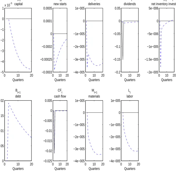
Figure 2 plots impulse response functions in the case of an i.i.d real interest rate shock. Note that in this case the dynamic responses of all variables are very similar to Figure 1 with the exception of labor. However, quantitatively the scale of the effect on the variables’ responses is orders of magnitude smaller than in the case of productivity shocks. The implications of this point are discussed below, but is worth pointing out that the reason is that an interest rate shock has a very small effect on firms’ dividends compared to the effect arising from a productivity shock. Evaluated at the steady state (impact effect on dividends), the coefficient on the interest rate equals (1

β −1)B = 0.0082, compared toK α

MγLν = 0.16 for productivity.15

4.1.2 The case of persistent shocks

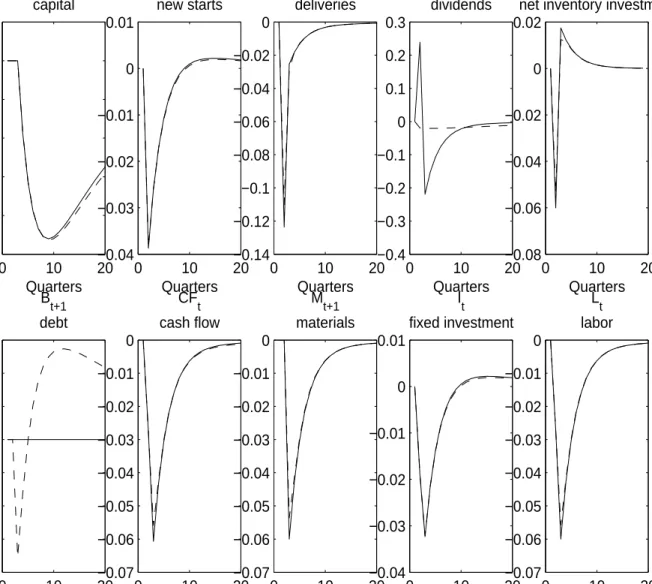
Examining the dynamic responses in the case of persistent productivity and interest rate shocks demonstrates that persistent shocks alone can produce similar dynamics with or without con-straints. Taking the case of productivity shocks, Figure 3 plots the dynamic responses, under the PCM case and constrained versions of the model for the baseline penalty parameters (Table 1).16

The most noticeable difference in the dynamic responses is on new project starts, s2t, debt,Bt+1,

dividends, divt, and the capital stock, Kt+1.17 Restricting attention to new starts, observe that in

the constrained version of the model the response—due to irreversibility—is orders of magnitude smaller relative to the PCM, where the firm is able to freely reduce the capital stock to its new (lower) optimal value immediately following the adverse productivity shock. In terms of the ratio of responses sP CM2t

sC

2t

= 264, contemporaneously. The implication is that new project starts (and fixed investment) are a lot more volatile than materials deliveries (sP CM2t

dP CM

t = 92) under PCM case. The

imposition of the constraints reverses this relationship making deliveries more volatile than new starts (sC2t

dC

t = 0.39, in the constrained version).

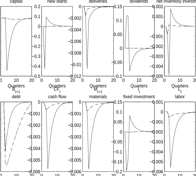
An additional difference arises in the dynamic response of debt, which can be illustrated with the aid of Figure 4. Relative to Figure 3, Figure 4 adds the responses with the irreversibility

14_{Debt responds nearly one-for-one with the productivity shock, i.e. 0.90 of the change in the productivity}

shock.

15_{Note that in the constrained version the firm hires less labor as the constraints imply that capital and}

materials will be lower in the future, making labor less productive. Also note that in this case labor does not respond contemporaneously, but only with lag (that is after the materials stock has been reduced in the period following the shock), and more interestingly the response is quite persistence compared to Figure 1. This latter property owes to the persistence of the capital and materials stock which remain below the frictionless level for many periods. Thus, in the interest ratei.i.dcase, labor becomes sensitive to financing constraints indirectly through the effect of these constraints on the productive assets of the firm.

16_{Beginning with this case fixed investment plots are presented, defined as in equation, (2.3).}

17_{Also note that in the constrained version, because capital is inefficiently high, factor use (materials and}

labor) is also higher relative to the PCM version, since the higher capital stock raises the respective marginal products.

constraint on new projects turned off (p2 = 0). The most noticeable change is on the dynamic

response of new starts, which absent the constraint can now be freely adjusted to allow the capital stock to reach the new (lower) optimum (notice that it nearly traces the response under PCM). The dynamic responses for the rest of the variables are very similar. This implies that the irreversibility constraint on new capital projects is largely responsible for the differences in dynamics, especially for the relative volatility of fixed and inventory investment. There is quite a noticeable difference in the response of debt. When there is no constraint ons2t, borrowing initially declines significantly

more compared to the baseline version (with all constraints active). Thus there is a trade off between adjusting debt and adjusting new project starts. When p₂ = 0, new starts decline freely in order to reduce the capital stock towards its new optimal (lower) value, and the firm reduces borrowing significantly in order to boost dividends in the next few future periods. The fact that the negative shock will persist and that materials and capital will be lower in the future (as a result of lower productivity) implies less income generated by production, and hence a decline in dividends which is costly since the constraint on dividends is active. The firm responds by reducing borrowing as this will reduce the future debt burden. But with the constraint ons2t active the capital stock declines

significantly less (as well as materials) which implies that the future loss in terms of dividends will be smaller, hence the incentive to cut borrowing today is reduced. Borrowing then reverses course and rises above the steady state as the firm wants to restore dividends to normal in later periods. As the productivity shock dissipates over time, capital, materials and labor rise towards the steady state values implying a higher production rate. But with the expenditure on deliveries and all projects recovered in the next few periods after the shock, dividends decline and borrowing then rises to boost current dividends in those later periods.

Figure 5 plots the dynamic responses with all but the irreversibility constraint shut off. By and large the most striking finding is the fact that compared to the PCM version there are hardly any differences in real variables’ dynamics. An important implication is that under persistent productivity shocks it is impossible to infer whether data on fixed investment are generated from the fully constrained version or the irreversible version of the model. This has important implications for empirical studies that attempt to detect capital market imperfections using fixed investment-cash flow regressions. In section 4.2 simulated data show that one will obtain nearly identical (positive) correlations from both versions of the model. This implies that in fixed investment (empirical) regressions a positive correlation with cash flow cannot be interpreted as evidence of capital market imperfections.

Finally, Figure 6 plots the dynamic responses in the case of a persistent (adverse) real interest rate shock. In the PCM version interest rate variation affects the cost of debt as well as the return

on fixed and inventory investment: a higher real interest rate implies that a unit of investment either in capital or inventories has a lower future return in terms of dividends. In other words the return to saving money (rather than investing inside the firm) has increased. This calls for lower investment in capital and inventories and as the productive assets of the firm decline leads the firm to hire less labor.18 _{The rise in the interest rate reduces current dividends and cash flow. The}

persistence of the shock implies that the future burden of any given debt load will be higher and will persist. Thus the firm reduces debt.

However, the effects compared to the productivity impulse are quantitatively small (compare the scales in Figures 3 and 6). Thus this analysis implies that pure interest rate variation is unable to produce the large impact effects of monetary policy on inventory investment as documented, for example in Gertler and Gilchrist (1994) or Bernanke and Gertler (1995). This finding is also consistent with the analysis in Maccini et al. (2004) on the lack of a significant short run effect of the real interest rate on inventory investment.

Comparing the dynamic responses under persistent interest rate and productivity shocks es-tablishes the claim in the introduction of the paper that under either type of shock procyclical materials deliveries and fixed investment do not necessarily imply financing constraints. Persis-tent shocks under PCM (with the irreversibility constraint alone) can give rise to procyclical fixed investment and materials deliveries. Thus, a researcher who is attempting to detect the presence of financing constraints needs to carefully condition any statement derived from cash-flow fixed investment correlations.

4.2

Second moments

Empirical studies that emphasize the role of capital market imperfections in explaining the cyclical behavior of inventories and fixed investment utilize panels of firms and typically regress inventory (fixed) investment to variables that proxy for these type of frictions. For example in Fazzari et al. (1988) or Carpenter et al. (1994) cash flow is the explanatory variable that aims to capture the im-pact of financing constraints in fixed investment and inventory investment regressions respectively; these authors demonstrate the significance of cash flow in explaining (fixed) inventory investment for a group of firms with imperfect access to capital markets. This section discusses the results obtained from the simulated model, concerning the validity of the conclusions from these studies. After simulating the model for persistent productivity (interest rate) shocks the problems that can

18_{As discussed in the previous section, the effect of the constraints on labor arise not because the firm finds}

it optimal to cut labor in order to save on internal funds but rather as a result of maintaining the optimal input mix (setting the marginal product of labor equal to the wage rate). Since capital and materials are declining so will labor to maintain the equality.

arise in interpreting cash-flow correlations are clear.

The calibrated version of the model is used to generate time series with 151 periods repeated 1000 times.19 _{This model can replicate firm histories with various degrees of financing constraints}

by adjusting the weight on the borrowing or equity constraint.

Tables 2, 3, 4 and 5 report contemporaneous correlations and illustrate several interesting results. First note that in either the baseline or PCM versions of the model (Tables 2 and 3), cash-flow, fixed investment are nearly collinear. Second, neither version is consistent with procyclical inventory investment as the correlations show. Third, they highlight the difficulties in correctly interpreting investment—cash flow correlations, an issue that only arises in the case of fixed invest-ment. Table 4 reports correlations obtained from a simulation of the PCM version of the model, with only the irreversibility constraint active. Table 4 verifies the analysis based on the impulse response functions. It shows that a strong positive correlation between fixed investment and cash flow does not necessarily reflect financing constraints. Note however that the correlation of inven-tory investment with cash flow is weakly negative which implies that inveninven-tory investment does not suffer from this problem. The reason can be most easily be explained with reference to Figure 5. The firm is attempting to reduce the capital stock in line with the lower productivity but is limited by the fact that it gets penalized as it reduces investment. Because capital is inefficiently high for this level of productivity, investment will remain below normal (relative to the steady state) for many periods. Since cash-flow and productivity shocks are highly positively correlated, cash flow will also be reverting slowly back to the steady state. As a result fixed investment and cash flow will be highly correlated. Materials deliveries on the other hand will immediately adjust in line with productivity and hence inventory investment will be below steady state only at the time of the shock. Thus, inventory investment will actually be falling when cash flow is rising.

Gomez (2001) makes a related point in a model of fixed investment with costly external finance. He emphasizes that reduced-form investment equations are likely to be mis-specified because the firm’s optimal investment policy function is highly non-linear and cash flow could be found to be important because (un-related to financing constraints) it can improve the quality of the linear approximation. In practice, researchers investigate the effect of cash flow after controlling for Tobin’s q. If Tobin’sq was measured without error then the addition of cash flow should not add any explanatory power, as according to Gomez (2001) theoretical simulations, the effect of financing constraints should be already included in the market value of the firm. Moreover because q and cash-flow are likely to be collinear, in the most relevant (empirical) scenario with measurement

19_{The sample under investigation is 1967Q2 to 2004Q4 due to availability of the inventory data from the}

Bureau of Economic Analysis. All simulations use the same sequence of shocks by fixing the seed for the random number generator.

error a researcher may find a role for cash flow in a reduced form regression that does not reflect financing constraints. In essence, Gomez’s result is driven by the high correlations between cash-flow, investment, productivity shocks, and Tobin’sq, just as in this model.

Finally, Table 5 reports the cross-correlations among the same set of variables when financing is very expensive.20 _{Clearly, in this case, a reduced form fixed investment regression is not a}

definitive test of the relevance of financing constraints. Notice that only when equity and debt financing become very expensive will a positive cash flow inventory investment correlation obtain. This implies that reduced form inventory investment, cash-flow regressions are a better way to test for the presence of capital market imperfections.

An important consideration is the fact that the constrained version of the model produces both contemporaneous and dynamic correlations between inventory and fixed investment that are closer to their empirical counterparts, compared to the PCM version. This is the subject of the next section.

4.3

Timing of responses

The finding that inventory investment leads fixed investment is an overlooked stylized fact that has not received a proper theoretical explanation. Tables 6 and 7 present contemporaneous and dynamic correlations of inventory investment by stage of fabrication and fixed investment in U.S. manufacturing.21 _{Two observations are worth noting. First, the lack of comovement between}

inventory and fixed investment contemporaneously is only a feature of input inventories. Second, inventory investment leads fixed investment. The maximum cross correlation for materials (MS) inventory investment implies a three quarter lead.

The model analyzed in this paper makes a precise prediction on the timing of the responses: inventory investment leads fixed investment. In the model, the reason for this difference is the presence of gestation lags, irreversibility for capital projects and the financing constraints. All of these features are necessary to produce this timing difference. For ease of exposition Figure 7 replicates the investment responses of the (time-to-build) versions of the model (TTB—baseline and tight financial constraints), along with the responses for a no-time-to-build (NTB) version of the model following an adverse productivity shock. Note that as the line (TTB and baseline) imply, time-to-build coupled with baseline penalties can only generate a one quarter lead. Without the time to build element (NTB), the maximum correlation obtains contemporaneously. By contrast

20_{This case is defined when p}

1 is increased to 0.067, and p3 to 0.5. The correlation signs are robust as

long as the penalty on borrowingp3>0.15. The remaining penalty parameters are as in baseline.

21_{The data on U.S. manufacturing investment are available only at an annual frequency. Quarterly}

esti-mates are obtained by interpolation on the higher aggregate (non-residential private fixed investment) using the Chow-Lin procedure.

only the version of the model with tight financial constraints can replicate the three quarter lead of materials inventory investment, by making the response of project starts hump shaped. In addition only this version can generate a positive cash-flow, inventory investment correlation, i.e., procyclical inventory investment (see Table 5).

The extra kick from financing constraints can be analyzed with the aid of Figure 8. The difference compared to the baseline case is evident in the behavior of debt, project starts and deliveries and can be explained by understanding how the tighter constraints affect the responses. When financing through equity is more expensive, debt (contemporaneously) declines less, since now a given reduction in dividends is more costly and the incentive to protect dividends is stronger.22

Because of the smaller reduction in debt, expenditure on project starts and materials deliveries declines by less contemporaneously compared to baseline. But at the same time the fact that it is very costly to borrow (compared to baseline) in future periods23 _{implies that other expenditure}

must protect liquidity (for dividend payments) in those future periods: since the equity constraint is now tighter, declines in dividends are penalized more. With capital inefficiently high for the level of productivity, the firm lets expenditure on new capital projects remain below normal for more periods (compared to baseline) and this action economizes on liquidity for dividend payments; moreover the response is hump-shaped, peaking a period after the shock.24 The fact that capital is inefficiently high (implying that money allocated to fund projects is less valuable compared to their use for liquidity) and borrowing is less effective in protecting dividends, provides the incentive to cut projects further in this period. This hump-shaped response along with the time-to-build feature generates the hump-shape response of fixed investment in Figure 7.25 26 _{The second half of Table}

7 presents the dynamic correlations calculated from the model. The model successfully replicates the maximum dynamic correlation that implies a three quarter lead of inventory investment.

Why is this a particularly attractive explanation for rationalizing the dynamic correlations in the data? Clearly one could argue that longer gestation lags, would predict a timing difference in

22_{Of course to a certain extent it is also due to the higher penalty attached to borrowing.}

23_{Recall from the discussion in section 4.1.2 that the firm borrows above normal in the future to boost}

dividends when expenditure has resumed to normal levels, but production rate is still below the steady state level.

24_{This is because fixed capital is slow depreciating compared to materials, hence deliveries have to revert}

more quickly to normal (compared to starts) to bring the materials stock to the level implied by productivity. In fact in simulations with a depreciation rate on capital above 10% quarterly, the response of starts becomes monotonic.

25_{Note that irreversibility is crucial for generating this response: it is the fact that fixed capital remains}

high, which makes expenditure on projects to remain persistently lower than normal.

26_{Also note that borrowing is not prohibitively expensive: borrowing still rises even though by much less}

compared to baseline. Moreover, this is not the only (penalty) parameter perturbation that can generate this timing pattern. Experimentation with other parameter configurations (as long asp3 >0.15) generates

this hump shaped response. These particular values were chosen because they maintain reasonable accuracy of the solution as defined in the Appendix.

accord with the data. While this is certainly true, a PCM version with irreversibility and gestation lags would not be consistent with the procyclicality of inventory investment, a key stylized fact of the inventory research. Similarly, one could also argue that irreversibility on deliveries of materials would produce the positive cash-flow inventory investment correlation. But in such case materials deliveries would not be as volatile compared to fixed investment, a finding against the empirical evidence as documented by Caggese (2007). Thus it is difficult for a PCM version of the model to be consistent with all the evidence.

5

Conclusions

This paper develops a rich decision theoretic model of investment in capital and inventories and uses it to study the cyclical behavior of fixed and input inventory investment. An overlooked empirical regularity is the fact that fixed investment lags inventory investment by a considerable length in business cycle frequencies. This fact has not received a theoretical explanation. This paper argues that this feature can be explained with a model that combines time-to-build for fixed capital, irreversibility and financing constraints. The model replicates successfully the dynamic empirical correlations observed in U.S. data. The appeal of this particular explanation owes to the fact that it can also generate a set of stylized facts from the inventory research. This is important because competitive explanations are not consistent with these facts. In particular, without financing constraints one cannot generate the procyclicality of inventory investment. The model’s formulation nests the perfect capital markets case and by comparison with the version with financing constraints, establishes the significance of financing constraints. Interestingly, financing constraints are not necessary to obtain procyclical materials deliveries and fixed investment. This implies that attributing procyclicality to financing constraints is incorrect. In empirical work, fixed investment—cash flow sensitivitiesdo not necessarily reflect financing constraints.

Since the model analyzes both productivity and interest rate shocks it provides a first pass at the quantitative importance of interest rate variation. This is important because this aids the understanding of the transmission mechanism of monetary policy from the perspective of inventory spending. The findings of the paper imply that interest rate changes can only generate a small fraction of the effects generated from productivity disturbances.

References

Abel, A. and Blanchard, O.: 1986, Investment and sales: Some empirical evidence,NBER working paper 2050.

Albuquerque, R. and Hopenhayn, H.: 1997, Optimal dynamic lending contracts with imperfect enforceability,RCER Working Paper 439, University of Rochester.

Basu, S. and Fernald, J.: 1997, Returns to scale in U.S. production: Estimates and implications,

Journal of Political Economy105, 249–83.

Bernanke, B. and Gertler, M.: 1995, Inside the black box: The credit channel of monetary policy transmission,Journal of Economic Perspectives 9, 27–48.

Bertola, G. and Caballero, R.: 1994, Irreversibility and aggregate investment,Review of Economic Studies61, 223–46.

Blinder, A. and Maccini, L.: 1991, Taking stock: a critical assessment of recent research on inven-tories,Journal of Economic Perspectives5, 73–96.

Boyd, S. and Vandenberghe, L.: 2004,Convex Optimixation, Cambridge University Press.

Caballero, R., Engel, E. and Haltiwanger, J.: 1995, Plant level adjustment and aggregate investment dynamics,Brooking Papers on Economic Activity pp. 1–54.

Caggese, A.: 2007, Financing constraints, irreversibility, and investment dynamics, forthcoming, Journal of Monetary Economics.

Carpenter, R., Fazzari, S. and Petersen, B.: 1994, Inventory investment, internal finance fluctua-tions and the business cycle,Brookings Papers on Economic Activity2, 75–138.

Fazzari, S., Hubbard, G. and Petersen, B.: 1988, Financing constraints and corporate investment,

Brokings Papers on Economic Activitypp. 141–95.

Gertler, M. and Gilchrist, S.: 1994, Monetary policy, business cycles, and the behavior of small manufacturing firms,Quarterly Journal of Economics 109, 309–40.

Gomez, J.: 2001, Financing investment,American Economic Review91, 1263–1285.

Hall, B. and Hall, R.: 1993, The value and performance of U.S. corporations, Brokings Papers on Economic Activitypp. 1–34.

Holt, R.: 2003, Investment and dividends under irreversibility and financial constraints,Journal of Economic Dynamics and Control27, 467–502.

Humphreys, B., Maccini, L. and Schuh, S.: 2001, Input and output inventories,Journal of Monetary Economics47, 347–75.

Kim, J., Kim, S. and Kollmann, R.: 2005, Applying perturbation methods to incomplete market models with exogenous borrowing constraints, Department of economics working paper, Tufts University.

Koeva, P.: 2001, Time-to-build and convex adjustment costs, Working paper 01/9, IMF.

Kydland, F. and Prescott, E.: 1982, Time to build and aggregate fluctuations, Econometrica

50, 1345–70.

Maccini, L., Moore, G. and Schaller, H.: 2004, The interest rate learning and inventory investment,

American Economic Review94, 1303–27.

Mayer, T. and Sonenblum, S.: 1955, Lead times for fixed investment, Review of Economics and Statistics37, 300–4.

Ramey, V.: 1989, Inventories as factors of production and economic fluctuations, American Eco-nomic Review79, 338–54.

Ramey, V. and West, K.: 1999, Inventories, in J. Taylor and M. Woodford (eds), Handbook of macroeconomics, Vol. 1B, Elsevier Science, North Holland, pp. 863–923.

Sakellaris, P. and Wilson, D.: 2004, Quantifying embodied technological change, Review of Eco-nomic Dynamics7, 1–26.

Schmitt-Grohe, S. and Uribe, M.: 2004, Solving dynamic general equilibrium models using a second-order approximation to the policy function,Journal of Economic Dynamics and Control28, 755– 775.

A

Solution

This section derives the equilibrium conditions of the model, describes the solution and defines the Euler equation errors to evaluate the accuracy of the approximation.

max Lt,s2t,dt,Bt+1 E0 ∞ X t=0   t−1 Y j=0 βj 

_{{divt+p1[divlog(divt)−divt] +p2[s2log(s2t)−s2t]} +p3[(B Lim 1 +r −B)log( BLim 1 +rt+1 −Bt+1) +Bt+1] +p4[dlog(dt)−dt]} s.t. div_t=A_tK_tαM_tγLν_t −wL_t−d_t−ϕ₁s_1t−ϕ₂s_2t+B_t+1−(1 +r_t)B_t Kt+1 = (1−δ)Kt+s1t s_2t=s_1,t+1 Mt+1 = (1−δm)Mt+dt lnA_t+1 =ρ_AlnA_t+σ_Aε_t+1 ε_t∼N(0,1) lnrt+1= (1−ρr)lnr+ρrlnrt+σrυt+1 υt∼N(0,1)

The Langrangean for this problem,

max Lt,s2t,dt,Bt+1 E₀ ½_X∞ t=0  tY−1 j=0 β_j 

_{{divt+p1[divlog(divt)−divt] +p2[s2log(s2t)−s2t]+}

p3[( B Lim (1 +r) −B)log( BLim (1 +r_t+1) −Bt+1) +Bt+1] +p4[dlog(dt)−dt]+ λ_t(K_t+1−(1−δ)K_t−s_2t−1) +µ_t(M_t+1−(1−δ_m)M_t−d_t)} ¾

The first order conditions associated with this problem are: w.r.tLt(labor)

(νAtKtαMtγLtν−1−w)[1 +p1(_divdiv

w.r.tdt (deliveries) −1 +p1(−_divdiv t + 1) +p4( d dt −1) +βtEt ½ At+1γKtα+1Mtγ+1−1Lνt+1[1 +p1(_divdiv t+1 −1)] +(1−δm)[1−p1(−_divdiv t+1 + 1)−p4( d dt+1 −1)] ¾ = 0 w.r.ts_2t (project starts) −ϕ2+p1ϕ2(−_divdiv t + 1) +p2(_ss2 2t −1) +βtEt ½ −ϕ1+p1ϕ1(−_divdiv t+1+ 1) + (1−δ)ϕ2−(1−δ)ϕ2p1(− div divt+1+ 1)−(1−δ)p2( s2 s2t+1−1) ¾ + βtβt+1Et ½ [At+2αK_tα₊₂−1M_tγ₊₂Lνt+2+ϕ1(1−δ)][1 +p1( div divt+2 −1)] ¾ = 0 w.r.tBt+1 (debt) 1 +p1(_divdiv t −1) +Et ½ p3(− BLim 1+r −B BLim 1+rt+1 −Bt+1 + 1) +βt(1 +rt+1)[−1 +p1(−_divdiv t+1 + 1)] ¾ = 0 A brief description of the intuition behind the optimality condition for materials orders follows. The Euler equation for materials orders describes the relevant trade-off the firm faces in adjusting orders. The firm can either order less materials today and enjoy the consumption value of higher dividends, or keep ordering at the same rate, and use these materials in production and enjoy higher dividends tomorrow. In response to an adverse shock today the firm must at the optimum equate the net benefit from reducing orders today to zero. Suppose for the moment that the constraints do not bind so that all thep_i terms vanish from the Euler equation. Then reducing orders by one unit today has a direct dividend value of 1 unit. But this same action has to be balanced against its future expected discounted cost in terms of the value loss given by the gross marginal product of materials, βtEt

½

At+1γKtα+1Mtγ+1−1Lνt+1+ (1−δm)

¾

. Incorporating the constraint on dividends means that there is an extra benefit of reducing orders today given byp1(−_divdiv_t + 1), i.e., the value

of moving away from the limit of the constraint. So in effect the total effect in terms of dividends today is given by−1 +p₁(−div

divt + 1), and now this has to be balanced against the future expected

discounted cost, βtEt

½

[At+1γKtα+1Mtγ+1−1Ltν+1+ (1−δm)][1 +p1(_divdiv_t+1 −1)]

¾

. It follows that the equity constraint makes materials orders more sensitive to the exogenous shocks of the model. Similarly, taking into account the effect of the constraint on materials orders changes the trade-off by the fact that it becomes costly to freely reduce orders since moving closer to the respective constraint limit is now penalized. On the other hand the future expected discounted cost is also

affected since an extra unit of un-depreciated materials implies extra slack of the constraint on orders in the future. This will have the effect of reducing the sensitivity of materials orders to the exogenous shocks of the model. Similar interpretations can be given for the remaining optimality conditions of the model.

Collecting all the equations that characterize equilibrium:

EtF(yt+2, yt+1, yt, xt+2, xt+1, xt) = 0 (A.1)

where xt denotes the vector of state variables and consists of capital, Kt, materials, Mt

half-complete projects, s1t, debt, Bt and the exogenous productivity, At, and interest rate, rt. The

vector yt consists of labor, Lt, materials orders, dt, and new projects, s2t. The solution to this

problem can be expressed as

yt=g(xt, σ)

xt+1 =h(xt, σ) +νσεt+1

whereν is a vector selecting the exogenous state variables, in this caseAt and rt, and σ = [σAσr]

To compute the second order approximation around (x, σ) = (x,0), one substitutes the proposed policy rules into (A.1) and makes use of the fact that derivatives of any order of (A.1) must equal to zero in order to compute the coefficients of the Taylor approximations of the proposed policy functions. The second order solution is completely characterized by the matrices that collect the first and second order derivatives of the policy functions with respect to the state variables and σ,

gx, hx, gxx, hxx, gσσ, hσσ.

These are evaluated at the deterministic steady state by setting σ = 0. The deterministic steady state can be completely characterized by solving thef.o.c0_{s settingA}

t=At+1 =E(A) = 1

and similarly rt = rt+1 = E(r) = r. Because steady state borrowing is indeterminate at the

non-stochastic steady state, steady state borrowing is set B = 1₄BLim_{, in line with the empirical}

evidence provided in section 3.1. Values forL, K, M can be easily derived which will be defined as non-linear expressions of the technology parameters (production and investment), discount factor, and depreciation rates. The rest of the steady state values (states and controls) can be expressed as functions ofL, K, M.

B

Computation of penalty parameters

The computational procedure below uses the following definitions for the three Euler equation errors.27

LetD1t=−1 +p1(−_divdiv_t + 1) +p4(_dd_t −1) S2t=−ϕ2+p1ϕ2(−_divdiv_t + 1) +p2(_ss₂2_t −1)

B3t= 1 +p1(_divdiv_t−1). Then following Jin and Judd (2002) define the unit free versions of the Euler

equation errors: w.r.tdt

EE1 = 1+ βtEt

½

At+1γKtα+1Mtγ+1−1Lνt+1[1 +p1(_divdiv_t+1 −1)] + (1−δm)[1−p1(−_divdiv_t+1 + 1)−p4(_dtd₊₁ −1)]

¾ D1t w.r.ts2t EE2 = 1+ β_tE_t ½ −ϕ₁+p₁ϕ₁(− div divt+1 + 1) + (1−δ)ϕ2−(1−δ)ϕ2p1(− div divt+1 + 1)−(1−δ)p2( s2 s2t+1 −1) ¾ S_2t + βtβt+1Et ½ [At+2αKtα+2−1Mtγ+2Lνt+2+ϕ1(1−δ)][1 +p1(_divdiv_t+2 −1)] ¾ S2t w.r.tBt+1 EE₃= 1 + Et ½ p3(− BLim 1+r −B BLim 1+_rt+1−Bt+1 + 1) +βt(1 +rt+1)[−1 +p1(−_divdiv_t+1 + 1)] ¾ B3t

The penalty parameterspi0_{s are computed according to the following procedure.}

1. Guess values for{p1, ...p4}. In the initial step use {p1, ..., p4}={0.01,0.01,0.01,0.01}.

2. Simulate the model for 100,000 periods (using the values in Table 1) and collect themin, and

max values for the state variables, (min, max)0.28

3. Define a grid for the state variables, that is (min, max)1 ⊇ (min, max)0, informed by the

(min, max) range from step (2) above and compute the three Euler equation errors associated with

dt, s2t, Bt+1. A 5nx size grid (nx = 6, the number of state variables) is used for the state variables

that is ± 10% away from the steady state.29 For the two shocks, At, rt a range defined by ±3

27_{Note that the static labor condition is not included. The reason is that the maximum approximation}

error from this equation is always less than the smallest error resulting from any the three Euler equations.

28_{The absolute maximum percent deviations away from the steady state is (2.78, 2.83) for s}

1t. For the rest of the state variables these are within 1% of the steady state.

29_{Since the range obtained from step (2) does not deviate considerably away from the steady state it seems}

standard deviations, σ_A, σr is used.

4. Define a grid for the four penalty parameters of sizenp4(where np = 5) and compute the

min-imum of the maxmin-imum Euler equation error for each point on the grid. The candidate optimal

{p1, ..., p4} are those that minimize the maximum Euler equation error.

5. Verify that the candidate optimal{p1, ..., p4} produce a (min, max) range, (min, max)2 for the

state variables that are consistent with the grid specified in step 3, i.e., (min, max)1 ⊇(min, max)2.

If yes, then these are the optimal{p1, ..., p4}. Otherwise repeat from step 2.

The Table below reports the maximum Euler equation errors calculated at the optimal values for the penalty parameters.

The conditional expectations are computed numerically using Gauss Hermite quadrature with 11 nodes. The errors reported are inlog10units. The units chosen imply that a -1 value represents

a $1 mistake for each $10 spent, a -2 value a $1 mistake for each $100 spent, etc. The maximum Euler equation error reported below imply roughly a 3$ mistake for each $1000 spent.

Table A1

Maximum Euler equation errors

max{log10(EE1), log10(EE2), log10(EE3)}

baseline (ρA, ρr) = (0.7,0.7) (ρA, ρr) = (0.7,0.0) (ρA, ρr) = (0.0,0.7) 5% -2.55 -2.70 -3.28 10% -2.35 -2.38 -3.17 tight constraintsa _(ρ A, ρr) = (0.7,0.7) (ρA, ρr) = (0.7,0.0) (ρA, ρr) = (0.0,0.7) 5% -2.10 -2.12 -2.15 10% -2.04 -2.06 -2.11 a_{Defined withp} 1= 0.067,p3= 0.5. Table 1 Calibrated parameters Technology Investment γ=0.5 ν = 0.2667 α=0.133 ϕ1=0.5 ϕ2=0.5

Depreciation Discount factor

δ=0.025 δm=0.5 β = ₁₊1_r = 0.99 r=0.95

Productivity process Interest rate process

σA=0.02 ρA= 0.7 σr=0.02 ρr = 0.71

Steady state debt Penalty parameters

Table 2

Correlations (baseline): persistent shocks

Variable ∆Mt+1 CF At rt It ∆Mt+1 1.00 -0.047 0.41 -0.01 0.07 CF 1.00 0.88 -0.02 0.94 At 1.00 -0.02 0.90 r_t 1.00 -0.10 It 1.00 Table 3

Correlations (PCM): persistent shocks

Variable ∆Mt+1 CF At rt It ∆Mt+1 1.00 -0.14 0.50 -0.04 0.99 CF 1.00 0.77 -0.04 -0.08 At 1.00 -0.02 0.53 rt 1.00 -0.07 I_t 1.00 Table 4 Correlations (PCM): PCM with irreversibility constraint: Variable ∆Mt+1 CF At rt It ∆Mt+1 1.00 -0.08 0.39 -0.01 0.05 CF 1.00 0.88 -0.02 0.94 At 1.00 -0.02 0.90 r_t 1.00 -0.10 It 1.00

Table 5

Correlations: expensive financingb

Variable ∆M_t+1 CF A_t r_t I_t ∆M_t+1 1.00 0.07 0.54 -0.02 -0.09 CF 1.00 0.82 -0.03 0.92 At 1.00 -0.02 0.72 rt 1.00 -0.03 It 1.00 b_{Defined withp}

1= 0.067,p3= 0.5. All others as in baseline. Table 6

Correlations (U.S.)– Cyclical component

Variable ∆M St ∆W Pt ∆F Gt M It

∆M St 1.00 0.51 0.59 0.05

∆W P_t 1.00 0.33 -0.01

∆F Gt 1.00 0.19

M It 1.00

Business cycle component calculated with Christiano-Fitzerald filter.

MS-materials and supplies, WP-work-in-progress.

T able 7 Cyclical beha vior of investment (fixed and inventories) U.S. d a ta (cyclical component) c Cross correlations of man ufacturing in vestmen t with: V ariable x x ( t − 5) x ( t − 4) x ( t − 3) x ( t − 2) x ( t − 1) x ( t ) x ( t + 1) x ( t + 2) x ( t + 3) x ( t + 4) x ( t + 5) ∆ M S 0.44 0.48 0.49 0.41 0.26 0.05 -0.18 -0.39 -0.52 -0.55 -0.47 ∆ W P 0.55 0.52 0.44 0.33 0.18 -0.01 -0.21 -0.41 -0.55 -0.61 -0.59 ∆ F G 0.23 0.28 0.33 0.35 0.31 0.19 -0.01 -0.23 -0.42 -0.54 -0.55 Model (cyclical component) d V ariable x x ( t − 5) x ( t − 4) x ( t − 3) x ( t − 2) x ( t − 1) x ( t ) x ( t + 1) x ( t + 2) x ( t + 3) x ( t + 4) x ( t + 5) ∆ M S 0.40 0.61 0.70 0.58 0.25 -0.18 -0.54 -0.68 -0.59 -0.39 -0.19 (0.20,0.57) (0.49,0.72) (0.61,0.78) (0.50,0.66) (0.19, 0.30) (-0.25,-0.11) (-0.63,-0.43) (-0.77,-0.57) (-0.70,-0.48) (-0.56,-0.21) (-0.40,0.05) c Cyclical comp onen t calculated with Christiano-Fitzgerald band pass filter. d Median values with 5 and 95 p ercen t bands.

Figure 1: Perfect capital markets (solid line) vs. Financial constraints (dotted line), i.i.d At

shock (response to one σA, deviations from steady state in percent)

0 10 20 −5 −4 −3 −2 −1 0 1x 10 −3 K t+1 capital Quarters 0 10 20 −0.03 −0.025 −0.02 −0.015 −0.01 −0.005 0 0.005 s 2t new starts Quarters 0 10 20 −0.004 −0.003 −0.002 −0.001 0 0.001 d t deliveries Quarters 0 10 20 −20 −15 −10 −5 0 5 div t dividends Quarters 0 10 20 −0.002 −0.0015 −0.001 −0.0005 0 0.0005 M t+1 − Mt

net inventory investment

Quarters 0 10 20 0 0.5 1 1.5 2 B t+1 debt Quarters 0 10 20 −3 −2.5 −2 −1.5 −1 −0.5 0 0.5 CF t cash flow Quarters 0 10 20 −0.004 −0.003 −0.002 −0.001 0 0.001 M t+1 materials Quarters 0 10 20 −3 −2.5 −2 −1.5 −1 −0.5 0 0.5 L t labor Quarters

Figure 2: Perfect capital markets (solid line) vs. Financial constraints (dotted line), i.i.d rt

shock

(response to oneσr, deviations from steady state in percent)

0 10 20 −5 −4 −3 −2 −1 0 1x 10 −5 K t+1 capital Quarters 0 10 20 −0.0003 −0.00025 −0.0002 0 0.0001 0.0005 s 2t new starts Quarters 0 10 20 −4e−005 −3e−005 −2e−005 −1e−005 0 1e−005 d t deliveries Quarters 0 10 20 −0.2 −0.15 −0.1 −0.05 0 0.05 div t dividends Quarters 0 10 20 −2e−005 −1.5e−005 −1e−005 −5e−006 0 5e−006 M t+1 �