Strategic Behavior and Collusion: An
Application to the Spanish Electricity Market
Ciarreta, Aitor and Gutierrez-Hita, Carlos
yUniversidad del Pais Vasco and Universitat Jaume I Castellon
October 20, 2004
Abstract
The paper has two major contributions to the theory of repeated games. First, we build a supergame oligopoly model where …rms compete in supply functions, we show how collusion sustainability is a¤ected by the presence of a convex cost function, the magnitude of both the slope of demand market, and the number of rivals. Then, we compare the results with those of the traditional Cournot reversion under the same structural characteristics. We …nd how depending on the number of …rms and the slope of the linear demand, collusion sustainability is easier under supply function than under Cournot competition. The conclusions of the models are simulated with data from the Spanish wholesale electricity market to predict lower bounds of the discount factors.
JEL: L11, L13, L51
Keywords: collusion, repeated games, electricity market
Address: Department of Economic Analysis II, University of the Basque Country, Avda Lehendakari Aguirre 83, Bilbao 48015. E-mail: jepciana@bs.ehu.es
yCarlos Gutierrez-Hita would like to thank his thesis adviser Ramon Fauli-Oller for his
helpful comments, and also Javier Alvarez in the econometrics and Maria Paz Espinosa in the theoretical sections. We are also grateful to all seminar participants at the Universidad del Pais Vasco, Unicersitat Jaume I Castellon, EARIE 2003 Conference, Young Spring Meeting at Brussels 2003 and XXVI-2004 Simposio at Pamplona. All possible errors remain under our entire responsability.
1
Introduction
It is well-known that collusive practices are prosecuted, because of the misal-location of resources that results from the output restriction and higher prices. Therefore, Antitrust laws explicitly prohibit coordination among …rms to reduce output, increase price, prevent entry, exclude actual competitors, and other practices that weakens competition.
Stigler’s classic (1964) paper already remarked that, the study of collusion in a static oligopoly model was very limited. Since his pioneer work, game theory has been widely used. Friedman (1971) proved that an oligopolistic su-pergame is a better approach to study collusion sustainability. Firms involved in those practices may …nd pro…table to deviate if the subsequent punishment is su¢ ciently small; that is, when the discount factor is close to one, then tacit collusion can support any Pareto Optimal outcome. Furthermore, the indus-trial organization literature aims to identify conditions that facilitate collusion, among them: product homogeneity, di¤erences among purchasers, fewness of sellers, high barriers to entry, vertical integration, and a low elasticity of de-mand. Thus, ceteris paribus, we should expect collusion to occur more often when these conditions are met1.
The supply function strategic oligopoly model has been widely developed by Klemperer and Meyer (1989). This approach relates the quantity a …rm sells to the price the market will bear: such a supply function allows the …rm to adapt better to changing conditions than does a traditional Bertrand competition (a commitment to a …xed price) or Cournot competition (a commitment to a …xed quantity). The Spanish Pool market resembles some of those characteristics: every day and for each hour, generators submit a supply schedule. Some ap-plications of the supply function approach to electricity markets can be found in Green (1992, 1996), Green and Newbery (1991) and Powell (1994) for the British case and in Baldick, and Grant and Khan (2000) for the California case. The paper has a …rst contribution to the theory of repeated games. We build a supergame-theoretic model to show how a convex cost function, the demand conditions, and the number of generators a¤ect the sustainability. of tacit collusion in those markets where …rms compete o¤ering supply schedules. Various authors have remarked that one important factor that may a¤ect the sustainability. of collusion is the elasticity of demand. Jacquemin and Slade (1989) note that ”the elasticity of the individual …rms demand curve is an important factor’a¤ecting the incentive to cheat by cutting price and increasing sales”. Collie (2003) develop a model using a constant elasticity of demand model to explain how elasticity a¤ects the sustainability of collusion in a Cournot framework.
We consider supply function competition for two main reasons. First, the-oretical literature on repeated games lacks this kind of competition structure to model collusion sustainability. Second, we are going to test the predictions 1Even the Spanish antitrust authority, Tribunal de Defensa de la Competencia, also
obtained from the theoretical model using data from the Spanish wholesale elec-tricity market, that, as we mentioned, resembles characteristics of that type of competition.
The paper also compares the model under SFC with the traditional Cournot model in which …rms compete o¤ering a single quantity-bid stretch. Such com-parison is done to explain two facts. First, these two approaches are mostly used to study electricity markets2. For example, Borenstein and Bushnell (1997) use
a Cournot simulation model to evaluate the performance of the California mar-ket. Ramos, Ventosa and Rivier (1998) also use a production-cost model under Cournot competition, that is relevant in the new regulatory framework of the electricity market, to provide a detailed representation of the electric system. The supply fuction approach is attractive because it o¤ers a more realistic view of electricity markets; at least o¤ers the possibility of developing some insight into the bidding behaviour of …rms. Second, if we use the slope of demand as aproximation of the elasticity of demand, we …nd that the conclusions about collusion sustainability signi…cantly di¤er from one model to the other.
We have two major theoretical …ndings. First, as we expected, both strategic approaches are sensitive to the slope of demand parameter. Our model predicts that when the slope of the linear demand is low enough, collusion is easier to sustain under SFC reversion than under Cournot competition reversion.
The paper is organized as follows. Section 2 is the set up of the stage game with …rms competing in supply functions. We do not consider strategic behavior on the demand side. The assumption is not so restrictive, since in the Spanish wholesale electricity market, distributors are vertically related to generators3.
Section 3 solves the supergame and get the predictions. Section 4 makes a comparison between the incentives to deviate from collusion under SFC reversion and under Cournot competition reversion. Section 5 provides empirical evidence using data from the Spanish wholesale electricity market, covering the period May 2001 to December 2003. We report estimates of the slope of demand, the elasticity of demand around the system marginal price, and the arch-elasticity of demand, under a linear speci…cation, then we simulate values of the discount factor for the two model speci…cations. Section 6 concludes and gives some policy recommendations.
2
The Stage-Game
We consider a market withnidentical and independent generators. Firms face both the cost of generation and the cost of transmission. We do not con-sider the problem of entry of new generators. The transmission network has a …xed capacity K, then each …rm gets a ki, the transmission quota, for the
generation and they pay the corresponding fee for access to the grid, so that
K=Pni=1ki.Therefore, suppose that each …rm minimizes the variable cost, for
2Borenstein, Bushnell, Khan and Stoft (1995) provide a general classi…cation of the di¤erent
markets and competitive equilibria in the electricity industry.
simplicity just the use of inputxat cost per unitr,
min rxi
s:a: qi=kipxi
Then xi = (qi=ki)2 and C(qi) = (r=ki2)q2i. Without loss of generality, we can
normalizer=k2
i =c=2( we abstract away from transmission congestions). Thus
the …nal speci…cation is,
Ci(qi) =
c
2q 2 i
The cost structure makes also explicit the fact that there are capacity con-straints in electricity generation and transmission, in contrast with most of the existing models, that assume constant marginal cost, but it does not address the problem of star-up costs because the cost function would be non-convex for some generation levels, and equilibrium may not be de…ned. The strategy for each generator is to o¤er a supply function de…ned as follows,
Si(p) = ip; i= 1; ::; n
with slope i, which is indeed the strategic variable of each …rm i. Observe how we impose a supply function that starts at the origin. Imposing a more general linear form likeSi(p) =Ai+ ipyields to the same conclusions since in
equilibrium Ai = 0 (See Greene, 1994, for a discussion on the solution to …rst
order linear di¤erential equations). Therefore the total supply of electricity at the wholesale market is given by,S(p) =Pni=1 ip.
We consider a linear demand function which is the sum of the demand bids of the former vertically related (before liberalization) distributors and independent retailers,
D(p) =s p
The demand has a non-zero x-intercept,s, that measures the size of the mar-ket, and a constant negative slope, 4. Firms simultaneously choose a supply
function to cover the market demand. There is a unique price at which market demand equals total supply5
n X i=1
ip=s p
Solving for p we can de…ne the equilibrium wholesale price in terms of the vector as,
p( ) = s
+Pni=1 i; where = ( 1; :::; i; :::; n)
4It is easy to show the positive relation between elasticity of demand, , and under a
linear demand speci…cation.
5Note that, given our assumptions this point is unique. Market demand is linear and
downward sloping inp. Supply functions for each …rmiis upward sloping inpso,Pni=1Si(p)
Therefore the pro…t function also depends on . Each …rmimaximizes pro…ts choosing i
max i
i( ) = ip( ) C[ ip( )]
The …rst order condition@ i( i; i)=@ iis,
[p( )]2+ i@[p( )] 2 @ i 1 i 2 1 2 i[p( )] 2 = 0; i= 1;2:::; n (1)
Solving for the system of …rst order conditions, we obtain the equilibrium value of the slope of the supply schedule,
SF (n; c; ) =(n 2) c +
2c(n 1) (2)
where =p(c +n)2 4(n 1)
We compare SF with the slope of the supply function under perfect competition (P C) where price equals marginal cost, and this is our measure of market power and the strategic interaction e¤ect among thengenerators in the market,
P C= 1
c
Clearly, as we expected, the inverse of the slope of the supply function under oligopolistic competition is smaller than the inverse of the slope of the supply function under perfect competition, for every n 1. Increasing the number of …rms enhances competition among participants, therefore individual supply function falls closer to marginal cost.
Lemma 1 In equilibrium, as SF becomes smaller, the pro…ts of the …rms are larger; that is,
@ ( SF)
@ SF <0
and the value of SF depend of the number of the …rms, (i) if n ! 1 then
SF
! P C, and (ii) if n = 1 then SF ! M, where M is the optimal strategy under monopoly outcome.
Proof. See appendix 2.
We summarize the properties of the supply function to changes in the other structural parameters( ; c); thus ceteris paribus:
Property 1 More price-response consumers, shifts up the supply function,
@ SF @ = 1 2(n 1) n+c 1 >0
If the consumers are more price-sensitive, given the size of the market, then non-competitive …rms compete for the existing customers by bidding lower every amount of output.
Property 2 Increases in the cost of production parameters shifts up the supply function
@ SF @c =
2 2
[(n 2)2+cn ] (n 2) 2 <0
An increase in the cost of production, due to for example more expensive in-puts or transmission access, will cause an increase in the slope of the oligopolistic supply function.
We report now the equilibrium price, quantities and pro…ts for each …rm,
qSF = [2(2n+c )] 1[2 +n+c ]ns
pSF = ns 2c n2+n(2 c + ) [2 (2n+c )] 1 SF = cs2[(n+c )2
+ (n+c ) 2n] 1
We can also …nd the e¤ect of changes in the structural parameters on the equilibrium pro…ts.
Property 1 More price-response consumers decrease pro…ts,
@ SF
@ =
(cs)2[n+c + ]2
[(n+c ) + (n+c )2 2n]2 <0 Property 2 Increases in the cost of production decreases pro…ts
@ SF
@c =
s2 3n3 (c )3+n2(7c 4) +n(5c2 2+ 4) (n(3n+ 2) c (4n+c ))
4 [2n+c ]2 <0
Recall that if consumers become more price-sensitives, then …rms respond by bidding lower, but it is not compensated by the reduction in the total consumer surplus available for the …rms, therefore the total e¤ect is a reduction in the pro…ts. Increasing cost as well as more intense competition, without changing consumer preferences, clearly shrink pro…ts.
3
The Supergame
We seek conditions for the sustainability of the most collusive outcome in the in…nitely repeated game. In the supergame a strategy must specify what action plays each …rmi at each periodt, so a strategy is de…ned by it. We assume generators play trigger strategies; all the …rms colude ( ) as long as there has been cooperation in the past (included herself), otherwise the punishment is to revert to supply function competition one period after the violation has been detected ( SF),
it=
if i = ; f or < t
SF
if i 6= ; f or < t (3) i= 1;2; :::; n; t; = 2; ::::;1
where is the optimal collusion strategy for each …rm. We suppose that all the …rms reach a collusive agreement which depend of the each supply function per …rm6, ( ) = Pn
i=1 i( i; i). Therefore, the cartel put in the market
a joint supply function, which is the sum of then(identical) individual supply functions. Therefore the problem can be written as,
max
f igni=1
( )
which yields a system ofn…rst order conditions of the form,
[p( )]2+ i @[p( )]2 @ i 1 i 2 i 2 [p( )] 2+ n X j6=i j 2 j 2 ! @[p( )]2 @ i = 0 (4) fori= 1;2; ::; n
We get the optimal symmetric strategy for the cartel participants,
=
n+c
We summarize the properties of the equilibrium slope of the supply function under collusion.
Property 1 Increases in the slope of the demand function shifts up the slope of the colluding supply function
@ @ =
n
(n+c )2 >0
Property 2 Increases in the cost of production parameters shifts down the supply function
@ @c =
2 (n+c )2 <0
Property 3 Increasing the number of …rms in generation reduces quantity bid for every price
@
@n = (n+c )2 <0
Increasing the number of …rms in the market also increases the number of the participants in the cartel agreement, therefore individual supply function shift further from the marginal cost since the pro…t maximizing level of output does increase in the same proportion.
6There are no incentives to form partial cartels, that is withk < nnumber of …rms, because
As we expected, the pro…t maximizing strategy restricts output, for every price, more than the oligopolistic level, therefore we get that
< SF < P C
The equilibrium price, quantity, and pro…ts for each …rm are given by,
p = s(c +n) (c + 2n) q = s c + 2n = s 2 2 (c + 2n)
The pro…t function for the colluding …rms behaves in the same way to changes in the structural parameters as the oligopolistic competition pro…t func-tion, namely it is decreasing when the slope of the demand function increases, decresing to increases in the cost function, and decreasing to the number of colluding …rms.
We look for values of the discount factor , such that the strategy is a Subgame Perfect Nash Equilibria (SPNE) for the repeated game. A path is sustainable by a SPNE if and only if it is sustainable by the penal code speci…ed (i.e. the in…nite reversion to the symmetric Nash equilibrium). At any stage
t >1, the choice of a supply schedule depends on the previous actions of the …rms. We compare the discounted value of the stream of pro…ts of collusion the pro…ts of deviation plus the in…nite sequence of discounted pro…ts under oligopolistic supply function competition. Pro…ts from deviation accrue when, under the trigger strategies, a …rm …nds, at a given stage, more pro…table to violate the agreement that sticking to it, despite of the reversion to competition in subsequent periods. A …rm by cheating puts in the market an individual supply function which is di¤erent form the agreed upon one in order to get extra pro…ts. Let us chooseias the deviator, the rest of the …rms believe that …rmimaintains collusion and stick to it. Call Di the optimal strategy obtained fromarg max i( i; i), where iis ann 1vector that speci…es that the rest
of the …rms remain under collusive supply functions. Firmisolves the following problem,
max i
[p( i; i)]2 1 12 i
The …rst order condition for optimization is,
[p Di ; i ]2+ @[p( D i ; i]2 @ Di ! 1 D i 2 ! 1 2 [p( D i ; i]2 = 0 (5)
Solving the equation we obtain the slope of the supply function for the deviator,
D= [2n+c 1]
As we expect it holds that the slope of the supply function of the deviator is between the collusion and the oligopolistic competition ones, i < Di < SFi .
Finally, the equilibrium price, quantities, and pro…ts are,
pD = [s n+ 2nc +c2 2 ][2n2 + 3nc 2+c2 3] 1
qD = [ns(2n+c 1)][2n2+ 3nc +c2 2] 1
D = s2(n+c )
2
2 (c + 1) (c + 2n 1) (2n+c )
It holds that the highest possible pro…ts are for the stage game when all the rivals collude and …rmi deviates, that is,
D> > SF > P C
The necessary and su¢ cient condition for the strategy pro…le to be SPNE of the in…nitely repeated game is,
1
1 >
D+ 1
SF (6)
equation [6] holds if,
> DD SF (7)
let us call the minimum value for the discount factor such that collusion is sustainable. We characterize in terms of the structural parameters in the following proposition:
Proposition 1 In the in…nitely repeated game, when …rms compete in supply functions , collusion is sustainable if , where
= 2(n 1)
2
g(n) +c2 2(1 +c2 2) (n+c )(1 +c )(c + 2n 1)
where g(n) is a polynomial function of grade 37. depends on the structural
parameters in the following way:
1. depends on the slope of the demand function,
@
@ > 0, if n <4 @
@ < 0, if n>4
for allc; n2R+
7The explicit form forg(n)is,
2. depends on the cost of generation in the same way of , @@ >0, ifn <4
and @@ <0, ifn>4.
3. depend positively on the number of …rms, @n@ >0; for all ; c2R+:
Proof. See appendix 2.
The …rst result is not apparently intuitive. Ifn <4 the model predicts that as the willingness to pay decreases, it also decreases collusion sustainability, that is when increases, the one-shot deviation gain( D )increases more than ( SF), then,
@( D )
@ >1
@( SF)
@ if n <4
so must increase for get the inequality to hold. The intuition for this result is the following: when there are few …rms in the market an increase in has a higher marginal impact on deviation pro…ts than in the in the punishment, be-cause supply function competition reversion with a low number of …rms implies a lower level of oligopolistic competition. As a result collusion sustainability is more di¢ cult and increases.
The result does not hold if n> 4. The reason is that if the oligopoly has more …rms an increase in decreases the incentive to cheat on the agreement. Two factors leads to this result: (i) …rst, the possibility of coordination is lower, due to the large number of …rms; (ii) second, a deviation gain when increase is lower than the subsequent punishment; then, ( D )does not compensate
the net present value of the stream of subsequent losses due to supply function reversion( SF); i.e. SFC is a severe punishment. Then,
@( D )
@ < 1
@( SF)
@ if n>4
so must decrease to get the equality8.
The result aboutcis explained in a simmilar way of . When the number of …rms and the cost are low is easy to sustain collusion because the extra pro…ts of a deviation are not to much in comparison with the subsequent punishment, but if the number of …rms rise andc is small a deviation is more pro…table because now, the pro…ts of the cartel must be divided betwen more …rms, however, the subsequent punishment is not several because all of us have an small c
parameter, so maintain collusion is di¢ cult (a high is expected). As the parametercincrease the punishment becomes more relevant in the former case, and the number of …rms plays an small role in the latter case, so the critical value of converges.
Increasing both the number of …rms and/or increasing the cost of production, also raise the cost of reaching an agreement and also the coordination problem is worsened. Under supply function competition, when is low, an increase in the
8It is esy to check that both, @( D )
@ >0and
@( SF)
number of …rms makes more di¢ cult sustain collusion because a deviation from collusion increases the one-stage pro…ts so as to compensate the punishment phase, for a wider range of the discount factor. But when the number of …rms is big enough, increases do not compensate the punishment in a wider range of the discount factor. As a result, for low values of an increase in the number of …rms has a great impact in , but the e¤ect is alleviated when ! 1. Then,
lim
!1
@ @n@ !0
4
Supply Function vs Cournot competition
We explore under what type of reversion, either SFC or Cournot competition, collusion is more easily sustainable. The motivation to compare both types of strategic interaction is related to the fact that a substantial amount of literature models electricity markets as a Cournot game (see [4], [12]). We are interested in the economic implications to use one or another market competition game for collusion sustainability. We showed in the previous section how a high willing-ness to pay together with a convex cost function facilitate tacit collusion when there is supply function competition reversion. On the contrary, we show how under Cournot reversion is more di¢ cult to sustain collusion when the market has the same structural conditions, regardless the number of …rms.
First, let us solve the model with the same market structure conditions but under Cournot competition. Now, the strategic variable for each …rm is quantity,
qi, so we consider the inverse demand function
p(Q) = 1(s Q)
where Q = qi+Pnj6=iqj. We compare the results of the stage-game and the
supergame under both types of strategic interaction.
4.1
The Cournot stage game
The equilibrium values of the symmetric equilibrium under Cournot competition (C) are9, qC = s c +n+ 1 pC = s(c +n) c 2+ (n+ 1) C = s2(2 +c ) 2 (1 +n+c )2
Even though …rms put just a single quantity in the market, for each price and given the supply of the others, the underlying supply function under Cournot
competition has slope,
C =
c +n
It is easy to check that SF < C< P C.
Under Cournot competition, …rms can choose only their quantities as a result of demand’s changes (measured by ) because they not have control on prices; but under Supply Function competition, …rms can make a simultaneous changes on quantities and prices in order to save pro…ts, because they have the ability of change both variables; as a result, Cournot …rms decrease equilibrium quantity lesser than Supply Function …rms, which o¤er a quantity-price pair in which: (i) quantity decrease more than under Cournot regime but; (ii) equilibrium price decrease lesser than under Cournot regime; saving more pro…ts.10
Proposition 2 In the one-shot game, an increase in the price-response of the consumers ( ), makes under Cournot competition bigger losses than under Sup-ply Function competition. Besides, quantity decrease more under SupSup-ply Func-tion competiFunc-tion than when …rms compete à la Cournot.
Proof. See appendix 2.
The intuition that underlies the proposition is that under supply function …rms are less sensitive to changes in than under Cournot competition because they have also can choose the price and not only the quantity as strategic vari-able. Increasing competition through more …rms in the market mitigates the result.
4.2
Collusion sustainability
We are interested in …nding the minimum value of the discount factor, , such that collusion is sustained under trigger strategies for the in…nitely repeated game. This strategy pro…le is standard in the literature (see, for instance Fried-man’1971). Formally, a strategy in the in…nitely repeated game is,
qi1=qicll qit= qcll if q i =qcll; f or < t qC if q i 6=qcll; f or < t ; i= 1;2; :::; n; t; = 2; ::::;1
We show that CT C solves the equation,
C =
DC cll
DC C (8)
where DC; C; cll are pro…ts under deviation from collusion, Cournot
compe-tition and collusion, respectively. Because of the convexity of the cost function, the critical value of the discount factor, depends on the structural parameters ( ; c; n).
Proposition 3 In the in…nitely repeated game with the …rms competing à la Cournot, the minimum value of the discount factor C such that collusion is sustainable is,
C= (n+c + 1)2
n2+n(4c + 6) + (2c2 2+ 4c + 1)
1. C depends negatively on the elasticity of demand, @@C <0
2. C depends positively on the number of …rms, @@nC >0
3. C depends negatively on the cost of production @@cC <0
Let us consider …rst the e¤ect of changes in the slope of the demand. As Friedman shows, when the marginal cost is constant the minimum discount factor to sustain collusion only depends onn. The convex cost function together with a low slope of demand, increases market power. Therefore, the extra pro…ts from deviation, are larger because the higher prices of the market. Considering that from the period + 1 ownwards the rest of …rms make Cournot-Nash competition, this punishment is not strong enough to dissuade …rms to cheat: …rms only refused to cheat if the elasticity of demand increase su¢ ciently. When elasticity rise, the incentives to deviate decrease become less attractive and,
@( DC cll)
@ < 1
@( cll C)
@ for alln
and the discount factor to maintain collusion must decrease. A symmilar result is showed by Collie, R. D (2003) in a model with constant elasticity of demand but without a cost speci…cation (assume zero marginal cost). A computational advantage of the Cournot framework is that constant elasticity demand curves are straightforward to represent, as in Borestein and Bushnell (1999). The ex-pression obtained is the same at Supply Function competition withn>4. This reveal to us that collusion sustainability about this two forms of competition, à la Supply Function and à la Cournot, are a¤ected in a di¤erent way by and
n. This merely a wide explanation.
Exploring the evolution of the discount factors and C, when we focus in the variations of the demand elasticity (measured in our model by ) under this two forms of competition, Supply Function and Cournot, we …nd that the values of to sustain collusion vary in a di¤erent way. When the number of …rms rise values of present a di¤erent evolution. The theoretical model suggest that when demand elasticity and the number of …rms is low, the sustainability of collusion is easier under Supply Function competition than under Cournot competition, but this result falls when the number of …rms rise and increases. The explanation and economic intuition of this result is the following. In a Cournot framework …rms have capacity to change quantities and, as a result, market price is obtained. In contrast, when …rms submit supply bids, they have the ability to change price and quantities for each and the ability to exploit
market power is high. For a reduce number of …rms cheating is lesser pro…table under Supply Function than under Cournot competition because the high value of the subsequent present value of the future punishments doesn’t compensate to cheat; as a result, …rms prefer to remain under collusion. This is true for all values of the elasticity of demand (values of ) ifn <6. On the contrary, when the environment is Cournot competition, the ability to exploit market power is lower but the subsequent punishment per period are lower too. This reason makes that, when elasticity of demand is low, put in the market a quantityqi+
by the deviator …rm generate an extra pro…ts which compensate competition à la Cournot from the rest of the periods. The main point is the ability to exploit market power and the severe of the punishment.
When elasticity of demand rise the result is a¤ected for the number of …rms. Rising number of …rms makes more easy collusion agreements under Cournot if is su¢ cient high. The reason for this fact is that market power losses under Supply Function are more severe than under Cournot so, D DC goes down as increase, so cheating is relatively less attractive under Cournot. Besides, the gap between C SF goes down more rapidly than DC D . Then, for
n>6there is a valuebin which collusion sustainability is equally probably to sustain under the two regimens. Finally, thisbvalue increase when the number of …rms and elasticity rise. More precisely,
Proposition 4 (i) When the number of …rms isn <6, for all values of it is easier to sustain collusion under Supply Function than under Cournot Competi-tion, so < C is hold; if the number of …rms isn>6, collusion sustainability is easier under Cournot than under Supply Function competition, i.e. > C (ii) besides, the value ofbdecrease with the number of …rms when rise,
@b @n@ <0
Proof. See appendix 2.
5
Empirical evidence: The Spanish Wholesale
Electricity Market
The aim of the empirical study is to check whether the Spanish wholesale elec-tricity market is, according to our theoretical predictions, conducive to collusive practices. The competition authorities already …led a case against the three ma-jor companies, Endesa (EN), Iberdrola (IB), and Union Fenosa (UF), charging for anti-competitive practices the days 19th, 20th and 21st of November 2001. The section is structured as follows. We brie‡y describe the rules of the market, which is administered as a pool. We continue with a description of the data. Then we estimate the demand functions for each time period after running a test of linearity. Finally we use those estimations to simulate values of the min-imum discount factor we obtained in the theoretical model as a function of the structural parameters under both types of oligopolistic reversion.
5.0.1 The Pool
The Spanish Wholesale Electricity Market is a mandatory pool (day-ahead mar-ket). It was created in 1998 (after the Law 54/1997). The pool works as follows. Before 11:00 am, quali…ed buyers and sellers of electricity present their o¤ers for the following day. Each day is divided into 24 periods, one for each hour. Sellers in the pool present o¤ers consisting of up to 25 di¤erent prices and the corresponding energy quantities, for each of the 24 periods and for each generat-ing unit they own; the prices must be increasgenerat-ing. An o¤er that no includes any restriction is called a ”simple o¤er”. However, a seller may present an o¤er with restrictions, according to the rules of the system, then it is called a ”complex o¤er”. At the same time quali…ed buyers present o¤ers11. Purchase bids state a quantity and a price of a power block and there can be as many as 25 power purchasing blocks for the same purchasing unit, with di¤erent prices for each block; the prices must be decreasing.
The system operator, OMEL, constructs, with the selling bids and the pur-chasing bids, an aggregate supply and an aggregate demand schedule respec-tively. In a session of the daily market, it combines these o¤ers matching de-mand and supply for each of the 24 periods and determines the equilibrium prices for each period (it is called the system marginal price) and the amount traded (market clearing quantity). This matching is the ”base daily operating schedule”, (PBF). After the PBF schedule is settled, the pool administrator evaluates the technical feasibility of the assignment; if the required technical re-strictions are met then the program is feasible; if not, some previously accepted o¤ers are eliminated and others included to obtain the ”provisional feasible daily schedule”, (PVP). This reassignment ends at 14:00. By 16:00 the ”…nal feasible daily schedule”, (PVD) is obtained taking into account the ancillary services assignment procedure. There is also an intra-day market to make any neces-sary adjustments between demand and supply12. The result is called the ”…nal
hourly schedule”, (PHF).
5.1
Descriptive Analysis of the Data
We have hourly data from May 2001 until December 2003, so there are overall 23401 hour-observations. Each hour-observation contains all the demand-bids by quali…ed agents and all the supply-bids by generators. The hours are clas-si…ed into peak, o¤-peak, and valley, to distinguish high demand, intermediate demand, and low demand hours respectively, following the market operator’s classi…cation.system (OMEL).
1 1From January 1st 2003, all buyers of electricity are considered quali…ed buyers. Before
that day quali…ed buyers were those with consumption greather or equal to 1 GWh per year.
1 2This intra-day market started working on April 1st, 1998. The …rst three monts it had 2
sessions per day; in 2002 has 6 sessions per day. The volume of energy traded is usually very low, around 2% of the total.
5.1.1 The Demand Schedule
We summarize the mean and the standard deviation of the following descriptive variables:
1. Block-bids: The number of price-quantity pairs submitted by a purchas-ing unit to the system operator.
2. Bidders: Number of demand-bidders for each hour-observation. They are distributors, external agents, quali…ed agents, retailers, and pumping stations.
3. Price-in‡exible demand segment: That is the horizontal segment of the demand schedule, which is at a price higher or equal to 17.99 cents of euro. The price-cap is 18.03 cents of euro.
4. Price: This is the weighted equilibrium price for each hour-observation as reported by OMEL, after including technical restrictions.
5. Quantity: This is the weighted equilibrium quantity for each hour-observation as reported by OMEL.
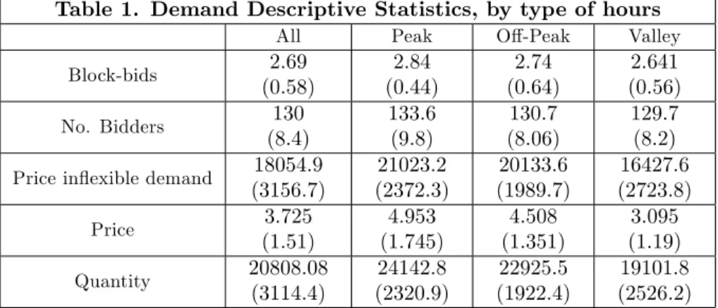
Table 1. Demand Descriptive Statistics, by type of hours
All Peak O¤-Peak Valley
Block-bids 2:69 (0:58) 2:84 (0:44) 2:74 (0:64) 2:641 (0:56) No. Bidders 130 (8:4) 133:6 (9:8) 130:7 (8:06) 129:7 (8:2)
Price in‡exible demand 18054:9
(3156:7) 21023:2 (2372:3) 20133:6 (1989:7) 16427:6 (2723:8) Price 3:725 (1:51) 4:953 (1:745) 4:508 (1:351) 3:095 (1:19) Quantity 20808:08 (3114:4) 24142:8 (2320:9) 22925:5 (1922:4) 19101:8 (2526:2)
It is noteworthy how the average number of block-bids is almost three (with a very low stadard deviation), regardless the type of hour, even though, by law, the maximum number of allowed bids is 25. Demanders facing uncertainty and very low real-time response consumers, bid as to get power so there are no disruptions in the service, therefore they have an incentive to bid high for most of the energy ther buy. As a result the price in‡exible demand amounts for 90 percent of the energy traded.
5.1.2 The supply schedule
There are four major …rms in the market that amount for the bulk of the total electricity generation
5.2
Linear demand speci…cation
We begin the empirical analysis with a test on the assumption of linearity of the demand. We estimate a demand function of the form,
Q(Pt) =s+ Pt +"t 8 < : If >1! concave If = 1! linear If <1! convex
where (s; ; ) are the parameters to be estimated. Thus if is signi…cantly close to one, we can proceed the analysis under a linear demand assumption. We estimate the demand functions corresponding to each hour of the entire data set using non-linear least squares (See Judge et al., 1985). Therefore, after the parameters’estimation, we have a time series for the exponentfbtg
T=23401 t=1 . We
run a test of means where the null hypothesis is the linearity of the demand function. The results reveal that on average = 1:015, however it is not signi…-cantly di¤erent from1. We also perform a test by type of hour, that is whether it is peak ( P), intermediate ( I) or low demand ( L) respectively. The test
is not rejected only during low demand hours, where L = 0:992. Still this
is just an average value, and this is precisely the target of our empirical study. This preliminary test should be interpreted as a starting point. It is not entirely clear that the aggregate demand schedule is approximately linear, specially dur-ing the year 2003. The variability in the estimation of the coe¢ cients is quite large, which explains the frequency of values di¤erent from1.
5.3
Slope of the Demand
We …t a linear demand function of the form,
Q(Pt) =s+ Pt+ tifPt 18:000
where the expected signs of estimation arebs >0andb<0respectively. Recall, there is a price cap atPt= 18:030, therefore not only equilibrium prices cannot
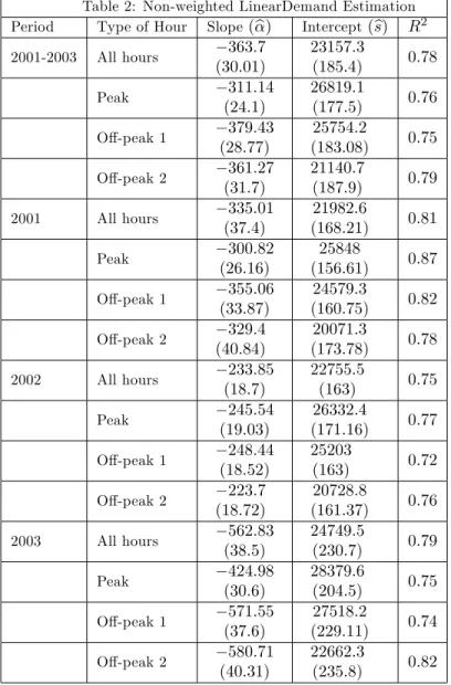
be above this level, but also price-dids are not considered. First, we report the non-weigthed average results in table 2 with the standard deviations into brackets. The price is measured in cents per KWh and the quantity in MWh.
Table 2: Non-weighted LinearDemand Estimation Period Type of Hour Slope(b) Intercept(bs) R2
2001-2003 All hours 363:7 (30:01) 23157:3 (185:4) 0:78 Peak 311:14 (24:1) 26819:1 (177:5) 0:76 O¤-peak 1 379:43 (28:77) 25754:2 (183:08) 0:75 O¤-peak 2 361:27 (31:7) 21140:7 (187:9) 0:79 2001 All hours 335:01 (37:4) 21982:6 (168:21) 0:81 Peak 300:82 (26:16) 25848 (156:61) 0:87 O¤-peak 1 355:06 (33:87) 24579:3 (160:75) 0:82 O¤-peak 2 329:4 (40:84) 20071:3 (173:78) 0:78 2002 All hours 233:85 (18:7) 22755:5 (163) 0:75 Peak 245:54 (19:03) 26332:4 (171:16) 0:77 O¤-peak 1 248:44 (18:52) 25203 (163) 0:72 O¤-peak 2 223:7 (18:72) 20728:8 (161:37) 0:76 2003 All hours 562:83 (38:5) 24749:5 (230:7) 0:79 Peak 424:98 (30:6) 28379:6 (204:5) 0:75 O¤-peak 1 571:55 (37:6) 27518:2 (229:11) 0:74 O¤-peak 2 580:71 (40:31) 22662:3 (235:8) 0:82
The estimation results reveal that, on average, the slope of the demand function is quite low, regardless whether the hour is peak, o¤-peak or valley. That is the demand is not price-responsive to changes in the price. In general, the goodness of …t is quite important, on average is around 80 percent. But, as demand grows it is becoming more price-responsive since more quali…ed agents are also becoming agents in the market without signing binding contracts with distributors.
5.4
Elasticity of Demand
We usebto compute estimations of the elasticity of demand around the system marginal price (SMP) as reported by the market operator. By de…nition, he elasticity of the demand,", at hourharound the system marginal price (Ph) is,
"h=
@Qh
@ph
Ph Qh
A local measure of the elasticity around the equilibrium is the arch-elasticity of demand. Let us consider Ph, and the market clearing quantity, Qh =
D(Ph). We take the highest price before the equilibrium price, Phhigh; such that D(Phhigh) < D(Ph), and the smallest price after the equilibrium price,
Plow
h , such thatD(Ph)< D(Phlow). The (absolute value of the) arch-elasticity
of demand, for hourh, is de…ned as,
"h= D(phighh ) D(plow h ) phighh plow h phighh +plow h D(phighh ) +D(plow h )
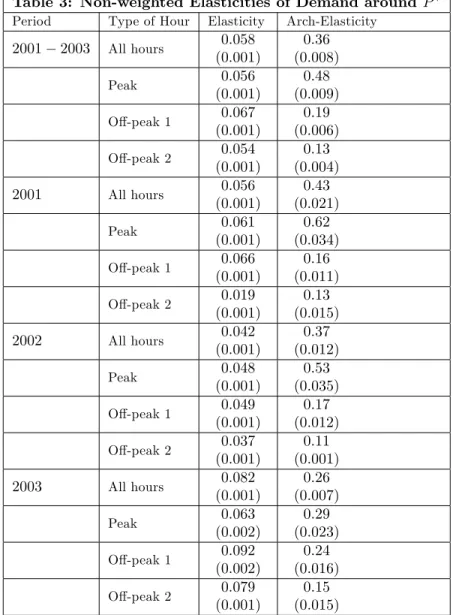
Table 3 reports the estimation results of both the elasticity of demand and the arch elasticity of demand.
Table 3: Non-weighted Elasticities of Demand aroundP
Period Type of Hour Elasticity Arch-Elasticity
2001 2003 All hours 0:058 (0:001) 0:36 (0:008) Peak 0:056 (0:001) 0:48 (0:009) O¤-peak 1 0:067 (0:001) 0:19 (0:006) O¤-peak 2 0:054 (0:001) 0:13 (0:004) 2001 All hours 0:056 (0:001) 0:43 (0:021) Peak 0:061 (0:001) 0:62 (0:034) O¤-peak 1 0:066 (0:001) 0:16 (0:011) O¤-peak 2 0:019 (0:001) 0:13 (0:015) 2002 All hours 0:042 (0:001) 0:37 (0:012) Peak 0:048 (0:001) 0:53 (0:035) O¤-peak 1 0:049 (0:001) 0:17 (0:012) O¤-peak 2 0:037 (0:001) 0:11 (0:001) 2003 All hours 0:082 (0:001) 0:26 (0:007) Peak 0:063 (0:002) 0:29 (0:023) O¤-peak 1 0:092 (0:002) 0:24 (0:016) O¤-peak 2 0:079 (0:001) 0:15 (0:015)
As we expected, the elasticity of demand is higher during peak hours than during the rest of the hours. Furthermore, as more quali…ed consumers enter the market, the demand schedule has more steps and becomes stepper. At the same time the arch elasticity of demand has reduced since there are more bolck-bids and the distance between D(phighh ); phighh and D(plow
h ); plowh is smaller.
5.5
Simulation values for
Finally, we simulate values for using thebestimations and for di¤erent number of …rms, n. We would also like to have estimations forc, but it is outside the
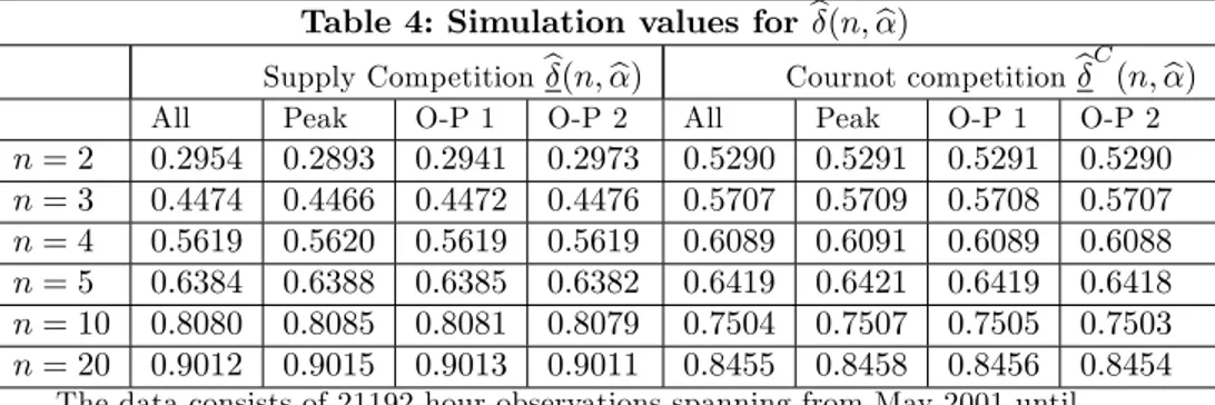
scope of the paper. We normalize c = 1, in the context of the model it is correct as long as we are not considering …rm asymmetries due to, for example di¤erent technology mix. Therefore we getb(n;b)as the estimated values for the lower bound of the discount factor such that collusion is sustainable using the estimations of the slope obtained in the previous section. We consider di¤erent values of the number of …rms under supply function competition and Cournot competition with increasing costs. The slope of the demand function has been normalized, in both cases, by the size of the market,s13.
Table 4: Simulation values forb(n;b)
Supply Competitionb(n;b) Cournot competitionbC(n;b)
All Peak O-P 1 O-P 2 All Peak O-P 1 O-P 2
n= 2 0:2954 0:2893 0:2941 0:2973 0:5290 0:5291 0:5291 0:5290 n= 3 0:4474 0:4466 0:4472 0:4476 0:5707 0:5709 0:5708 0:5707 n= 4 0:5619 0:5620 0:5619 0:5619 0:6089 0:6091 0:6089 0:6088 n= 5 0:6384 0:6388 0:6385 0:6382 0:6419 0:6421 0:6419 0:6418 n= 10 0:8080 0:8085 0:8081 0:8079 0:7504 0:7507 0:7505 0:7503 n= 20 0:9012 0:9015 0:9013 0:9011 0:8455 0:8458 0:8456 0:8454
The data consists of 21192 hour observations spanning from May 2001 until September 2003
We can conclude from the analysis of the demand of the Spanish electricity wholesale market that three structural characteristics could play an important role in the favor of collusive practices. One is the form of the competition à la Supply Function, which, despite the limitations of the model, we believe it is a better representation of the strategic interaction than Cournot or Bertrand competition. The second is about the nature of the demand curve, it is highly inelastic. The third one is the reduce number of …rms.The following corollary summarize the results.
Corollary 1 Collusive practices in electricity markets are easier to arise when the following conditions hold
the form of the competition is in supply functions as compared to Cournot. the demand curve is steeper.
the number of …rms is small.
5.5.1 Policy recommendations
Advocates of the Spanish Electricity Market restructuring argue that it should increase production and consumption e¢ ciency, by promoting competition among
1 3The reason for this normailzation is that the intercept in the X-axis and Y-axis are
a¤ected bys. Divided the demand function speci…ed we obtain qs= 1 spwhere qs 2[0;1] and the values of become relevant.
generators. We show how, besides the supply-side studies reviewed in the intro-duction, demand-side rigidities may actually be welfare-worsening, since …rms …nd easy to sustain collusive outcomes. Therefore, price-cap regulation when the price is set in the neighborhood of the marginal cost, is more desirable. The theory of demand-side price incentives is developing mechanisms to make demand more responsive towards price variability14. The problem to solve is
how to get a more active demand in the electricity market. Some contractual …gures could be implemented. Static time-varying prices, which are preset for determined hours and days, are actually not that di¢ cult to implement since a classi…cation of demand hours is available, and accordingly di¤erent tari¤s. Dynamic time-varying prices are similar in nature, but are allowed to vary within short notice. The main barrier is to make information available to …nal consumers on the bene…ts of the use of these type of tari¤s. For that reason in-dependent electricity retailers is a prerequisite, and break the vertically related tights among generators and distributors.
6
Conclusions
The paper has two major contributions to the literature. First, it is a con-tribution to the theory of repeated games, and second, another application to the empirical studies on electricity markets. First, we develope a supergame-theoretic framework for …rms that compete in supply functions; we evaluate collusion sustainability under this form of competition and for a certain market structure. We have shown how tacit collusion is easier to sustain as the will-ingness to pay for the good, given the size of the market, increases, and …rms compete in supply functions. These results are in contrast with the traditional Cournot framework: Collusion is more di¢ cult to sustain.
Second, we simulate the theoretical model with data from the Spanish Whole-sale Electricity Market. Empirical evidence shows that if the Spanish pool can be modeled as a supply function competitive market, …rms could sustain tacit collusion in a wide range of the discount factor. The result has to be inter-preted carefully since we just point out there are characteristics of the market that facilitate collusion, but the nodel is unable to detect actual collusion.
1 4For a survey on the literature of demand-side incentives, see Borenstein et al., UCEI-WP,
7
Appendix 1: Further Calculations
7.1
Supply Funtion Competition
JOINT-PROFIT CARTEL:The joint pro…t function is,
( i; i) = (n 1) i+ i ( + (n 1) i+ i)2 c(n 1) 2 j + (n 1) i+ i 2 c 2 i + (n 1) i+ i 2
therefore. there aren…rst order conditions
@ COL(
i; i)
@ i =
s[ i(c + 1) (c i+ 1)(n 1) i+ (n 1)c i] ( + i+ (n 1) i)3
imposing symmetry i= i= and solving for we obtain
=
n+c
PROFITS FROM DEVIATION: Given the equilibrium price and quantity for the colluding …rms, there is an incentive for deviation since the marginal revenue is above the marginal cost for each …rm. Thus the …rst order condition is,
@ i( i; i)
@ i =
s2(n+c )2[(c2 2+ 2nc +n) i (c + 2n 1) ] [(n+c ) i+ (c + 2n 1) ]3
solving in i(assuming symmetry) we obtain the optimal supply function for a potential deviator,
D
= [c + 2n 1]
c2 2+ 2nc +n
SUPPLY FUNCTION REVERSION: If competition occurs, then …rst order condition for each …rm is,
s2 i +c i+ (c i 1)(n 1) i + i+ (n 1) i 1= 0
solving in we obtain the optimal strategy SF for each …rm,
SF = [2c(n 1)] 1h
(n 2) c + ((c +n)2 4(n 1))1=2i
Replacing SF in the price expressionp( SF), we obtain
7.2
Cournot Competition
JOINT-PROFIT CARTEL:The joint maximization problem is
max fqigni=1 (q1; ::; qi; ::; qn) = n X i=1 i(qi; q i)
withn…rst order condition for interior solutions,
1q i+s 1 1[qi n X j6=i qj] cqi= 0; i= 1;2; ::; n
impose symmetry we obtain collusion quantity for each …rm,
qcll= s
c + 2n
replacing in the demand function, we obtain collusion price,
pcll=s(c + 2n 1) (2n+c )
and the pro…ts for each …rm are,
cll= s2 4n + 2c 2
PROFITS FROM DEVIATION: …rm i is the deviator …rm. Firms labelled iremain producing collusion quantitiesq i. The maximization problem for the deviator …rm is
max qi Cd(q i; q i) = [s 1 1(qi+ (n 1)q )]qi c 2q 2 i
with …rst order condition for interior solutions,
1q
i+s 1 1[qi (n 1)q ] cqi= 0
Solving we obtain,
qCd= s(n+c + 1) (2 +c )(2n+c )
thus the expressions for the rest of the endogenous variables are,
pCd = s(c
2 2 3 +n(3 + 2c )) (2 +c )(2n+c ) Cd = s2(1 +n+c )2
COURNOT REVERSION:The maximization problem for each …rm iis max qi C i (qi; q i) = [s 1 1(qi X i6=j qj)]qi c 2q 2 i
where q i is the vector with the strategies of the restj 6=i …rms. First
order condition for interior solutions,
1(2 +c )q
i 1[(n 1)qj s] = 0
under symmetry across …rms,
qC=s[c +n+ 1] 1 pC= s(c +n) c 2+ (n+ 1) C= s2(2 +c ) 2 (1 +n+c )2
8
References
References
[1] Allaz, B., Vila, J-L. (1991).”Cournot Competition, Forward Markets and E¢ ciency”. Journal of Economic Theory, vol 59, 1-16.
[2] Baldick, R., Grant, R and Kahn, E. (2000).”Linear Supply Function Equi-librium: Generalizations, Application, and Limitations”. POWER, PWP-078.
[3] Bolle, F.(1992).”Supply Fuction Equilibria and the Danger of Tacit Collu-sion: the Case of Spot Markets for Electricity”, Energy Economics, 94-102. [4] Borenstein, S., Bushnell, J.(1999). ”An empirical analysis of the potential for market power in California’s electricity industry”. Journal of Industrial Economics 47(3), 285-323.
[5] Borenstein, S., Bushnell, J., Khan, e., Stoft, S.(1995).” Market Power in California electricity markets”. Utilities Policy 5 (374), 219-236.
[6] Collie R. D, (2004). ”Collusion and the elasticity of demand” Economics Bulletin, Vol. 12, No. 3 pp. 1-6.
[7] Day, C., Hobbs, B., and Pang, J-S.(2002).”Oligopolistic Competition in Power Networks: A Conjectured Supply Function Approach”, POWER, PWP-090.
[8] Fabra, N. (2003).”Tacit Collusion in Repeated Auctions: Uniform versus Discriminatory”, Journal of Industrial Economics, Vol. L1, No. 3 (Septem-ber), pp. 271-293, 2003.
[9] Green, R.(1999).”The Electricity Contract Market in England and Wales”. The Journal of Industrial Economics, vol XLVII, 107-124.
[10] Green, R.(1996).”Increasing Competition in the British Electricity Spot Market”. The journal of Industrial Economics, vol XLIV, 205-216.
[11] Green, R.(2001).”Failing Electricity Markets: Should we shoot the Pools?”. Working Paper, University of Hull.
[12] Jacquemin, A and Margaret E. Slade, (1989). ”Cartel, Collusion, and Hor-izontal mergers” in Handbook of Industrial Organization, Vol 1, North Holland, Amsterdam.
[13] Klemperer, P. and Meyer, M.(1989) ”Supply Function Equilibria in Oligopoly Under Uncertainty”. Econometrica. vol 57, no 6, 1243-1227.
[14] Ramos, A ,Ventosa, M., and Rivier, M.(1998).”Modelling Competition in Electricity Energy Markets by Equilibrium Constraints”. Utilities Policy, vol 7,no 4, 223-242.
[15] Powell, A.(1993).”Trading Forward in an Imperfect Market: The case of Electricity in Britain”. The economic Journal, vol 103, 444-453.
[16] Selten, R., "A Simple Model of Imperfect Competition When 4 Are Few and 6 Are Many", International Journal of Game Theory 2 (1973), 141-201 [17] Stoft, S, Power Market Economics: Designing Markets for Electricity",
Wiley & Sons, 2000
[18] Wolak, F. A. (2003). ”Measuring Unilateral Market Power in the Wholesale Electricity Markets: The CAlifornia Market, 1998-2000”. AEA Papers and Proceedings, vol 93, NO. 2. May 2003, 425-430.
9
Appendix 2: Proofs
PROOF OF LEMMA 1. We are going to proceed in two steps. First, we proof the chain P C > SF > M. When1< n <1we obtain SF as a result of the pro…t maximization of the …rm’s pro…ts. Whenn! 1
we expected to obtain the result of perfect competition15; then,
lim n!1 (n 2) c + 2c(n 1) = 1 1
1 5This result is hold …xing exgenouslyp; then,
max i
i( ) = ip C[ ip]
dividing both, numerator and denominator withnwe obtain lim n!1 "(n 2) c n +n 2c(nn1) # =1 c
Whenn!1we expected to obtain the result of a monopoly16; then,
lim n!1 (n 2) c + 2c(n 1) = 1 1
numerator and denominator are derivables so applying L’Hopital’s theo-rem we obtain an equivalent limit
lim n!1 (1 +
c +n 2
)=2c = 1 +c
if we solve the lateral limitn!1+ with1+= 1 +"we obtain, lim
n!1+
(n 2) c +
2c(n 1) =1 "+c
then, if n > 1 we …nd that SF > M. Of course, 1c > 1 "+c )
1 "+c > c )1> because !0. As a result P C > SF > M. In the second, we want to proof that
@ ( SF)
@ SF =
s2( (n+c ) SF) ( +n SF)3 <0
the denominator is always positive ands2 too. Then,( (n+c ) SF)
must be less than zero, or n+c < SF. We know that SF > M = 1+c > n+c , so
SF
>n+c . This complete the proof.
PROOF OF PROPOSITION 1. Let us normalizec= 1. The expres-sion for is obtained by substituting pro…ts of collusion ( COL), deviation
( DEV) and supply function competition ( SF). These three pro…t
func-tions depend on the number of …rms and the slope of demand function, then the right hand side of equation [7] can be written as
( ; n) =
D( ; n) ( ; n) D( ; n) SF( ; n)
taking the partial derivate respect to we get,
@ ( ; n)
@ =
4(n 1)2( 2 + 6n n2 2n3+n4+ 10n 8n2 + (2n3 3n2+ 2n+ 2n + 2n3 + 2+ 5n2 2+
1 6This result is hold by …xingn= 1and
max ( ) = p( ) C[ p( )]
+6n3 + 5 2 4n 2+ 11n2 2+ 8n 3+ 2 4 (n+ ) (1 +n2+ 4n + 2)) +4n 3+ 4+ (1 + )(n+ )(2n+ 1) )2
We are interested in the sign of the e¤ect. The denominator is always positive. In particular, we want to know when this polynomial function change the value. Then, making it equal to zero and solving in , we get an expression that depends onn. Let us rename the expression as (n),
(n) =
p
(n 1)3
p
(n 3)p2 n
The function (n)takes positive values forn <4and negative values for the rest.
PROOF OF PROPOSITION 2. This proof has two parts. We can eliminate s2 from the expressions of C , SF , qC and qSF and makes
c = 1 because the e¤ect of this parameter in pro…ts is the same of the one, and cualitative result are mantained. First, we prove that an increase in the price-response of the consumers ( ) makes under Cournot competition bigger losses than under Supply Function competition. Then we are interested in the value of @@C and @@SF. The values of the partial derivates are, @ C @ = 3 + 2+n+ 1 2( +n+ 1)3 @ SF @ = ( +n+ )2 [(n+c )2+ (n+c ) 2n]2
This two expressions are always negative. Finally, we are interested to show that @@C @@SF 0, that is,
[3 + 2+n+1][(n+ )2+(n+ ) 2n]2 2( +n+1)3( +n+ )2 0
for all values of andn. Second, we prove that quantity decrease more un-der Supply Function competition than when …rms compete à la Cournot. Then, we are interested in the value of @q@C and @q@SF. The values of the partial derivates are,
@qC @ = 1 ( +n+ 1)2 @qSF @ = n(n2+n(4 + ) + 2( 2)) 2( + 2n)2
This two expressions are always negative. Finally, we are interested to show that @ C
@
@ SF
@ 0, that is,
2( + 2n)2 n(n2+n(4 + ) + 2( 2))( +n+ 1)2 0
for all values of andn. This complete the proof. Note: upon request, we report an extension of the proof with calculus and gra…cs with the Mathematica Program.
PROOF OF PROPOSITION 3.Let us normalize c = 1: From the expressions [7] and [8] we are interested to check when both expressions are equal. Taking the right hand side,
Cd+ 1 C ? = D+ 1 SF
It could be equal when Q! ; let us call this valueb. Then,
D Cd= b
1 b(
C SF) (9)
The intuition of the equation is the following: when the gap of the de-viation’s pro…tability between Supply function and Cournot is equal to the discounted gap between Cournot and supply function reversion, col-lusion under Cournot and supply function are equally sustained. Solving equation [9],
b= (
D Cd)
( D Cd) ( C SF)
when n < 6 there isn’t any value of b 2 (0;1) which can balance the equation. For values n>6we …nd a positive relation between , n, and
b. That is,
@b @n@ =
2(n 1)(n3 13 26 18 2 4 3 n2(2 + 7) n(13 + 20 + 6 2)) (1 +n2+ 4 + 2 2+n(6 + 4 ))3 >0