The dynamics of international asset price linkages and
their effects on German stock and bond markets
Dietrich Domanski and Manfred Kremer
11.
Introduction
The financial market turbulences in 1998, as other crises previously, produced strong price movements in the securities markets worldwide. This reflected, first, a general reassessment of credit risk, and, second, a drying-up of liquidity even in some of the largest mature securities markets.2 As a result, cross-market return correlations temporarily underwent dramatic changes, challenging portfolio allocation and risk management strategies which rely on constant historical comovements of asset prices. Against this background, the immediate question arises of how asset price linkages can be properly measured when they are subject to periodic changes as observed in times of market stress. The main purpose of the present paper is to address this question more thoroughly.
In order to measure the dynamics of international asset price linkages, we first employ bivariate GARCH models to analyse the comovements between weekly stock and bond market returns across the G3 countries. GARCH models take account of the specific time-series properties of short-term asset returns, which is needed to obtain reliable estimates of the cross-country linkages. Next, switching-regime ARCH or “SWARCH” models are applied which can identify different volatility regimes for short-term asset prices endogenously. We use this methodology to address two issues: first, “Are international short-term return linkages state-dependent?”, and second, “Do volatility spillovers affect individual segments of the domestic bond or stock market differently (i.e. are they market-segment-dependent)?” The first question may also be referred to as the “contagion hypothesis”. This states that contagion leads to a significant increase in the cross-market correlation during states of financial market turmoil. Hence, contagion differs from mere “interdependence” in that it demands a stronger-than-normal market linkage during periods of stress.3
The paper is organised as follows: Section 2 presents some stylised facts on short-term asset returns derived from summary statistics and simple cross-market correlations. In the third section, we outline the ARCH and SWARCH techniques employed to assess the comovements of weekly returns on various bond and stock price indices. In Section 4, the hypothesis of state-dependent international volatility spillovers between the United States, Japan and Germany is tested. The fifth section examines the question of market-segment-dependent contagion within the German financial system. Section 6 concludes by addressing some possible implications of the results.
2.
Measuring international asset price linkages: some stylised facts
The asset universe considered in this paper comprises G3 bond and stock markets, the former represented by the prices of 10-year benchmark government bonds, the latter by broad-market price indices of Datastream (DS country indices).4 Additionally, the following segments of German
1
The views expressed in this paper are those of the authors and do not necessarily reflect the opinion of the Deutsche Bundesbank.
2
See International Monetary Fund (1998), p. 38.
3
See Forbes and Rigobon (1999), p. 1, and Baig and Goldfajn (1999), p. 169.
4
financial markets are analysed: in the bond market, different maturities for benchmark government bonds (besides the year maturity, also two, five and seven years), as well as the price index for 10-year Pfandbriefe (“PEX”) are considered. The stock market is broken down into the blue chips contained in the DAX, and a segment for medium-sized and small stocks, respectively (MDAX and SMAX).5 Asset price movements are measured as weekly returns, based on Thursday figures for Germany and Japan. For the United States, Wednesday figures are used, taking into account the asynchrony between these markets with the US market performing a lead function for the others.6 The stock market data cover the period from January 1980 (MDAX and SMAX: October 1988) until September 1999. The bond market sample ranges from January 1984 (PEX: January 1988) to September 1999.
Table A1 in the Appendix shows some univariate summary statistics for all time series of weekly asset returns analysed in this paper. Over the entire sample period, stock markets generate higher, less autocorrelated and more volatile returns than bond markets do. Despite these marked differences, both asset classes share many other features typical of higher-frequency asset prices. First, returns exhibit substantial non-normality (as can be seen from the Jarque-Bera statistic) which mainly stems from excess kurtosis. That is, the distributions of short-term returns are characterised more by fat tails than by asymmetry (skewness). Moreover, autocorrelation is generally low and often insignificant. Finally, ARCH tests reveal strong volatility clustering in bond and stock returns. These properties suggest using a time-series framework for modelling short-term asset returns which captures serial correlation in the conditional means and variances, and which generates unconditionally leptokurtic, but not necessarily skewed returns.
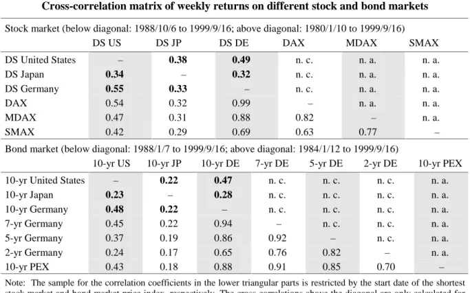
Table 1
Cross-correlation matrix of weekly returns on different stock and bond markets
Stock market (below diagonal: 1988/10/6 to 1999/9/16; above diagonal: 1980/1/10 to 1999/9/16)
DS US DS JP DS DE DAX MDAX SMAX
DS United States – 0.38 0.49 n. c. n. a. n. a. DS Japan 0.34 – 0.32 n. c. n. a. n. a. DS Germany 0.55 0.33 – n. c. n. a. n. a. DAX 0.54 0.32 0.99 – n. a. n. a. MDAX 0.47 0.31 0.88 0.82 – n. a. SMAX 0.42 0.29 0.69 0.63 0.77 –
Bond market (below diagonal: 1988/1/7 to 1999/9/16; above diagonal: 1984/1/12 to 1999/9/16)
10-yr US 10-yr JP 10-yr DE 7-yr DE 5-yr DE 2-yr DE 10-yr PEX 10-yr United States – 0.22 0.47 n. c. n. c. n. c. n. a.
10-yr Japan 0.23 – 0.28 n. c. n. c. n. c. n. a. 10-yr Germany 0.48 0.22 – n. c. n. c. n. c. n. a. 7-yr Germany 0.45 0.22 0.94 – n. c. n. c. n. a. 5-yr Germany 0.37 0.19 0.86 0.92 – n. c. n. a. 2-yr Germany 0.24 0.17 0.65 0.76 0.82 – n. a. 10-yr PEX 0.43 0.18 0.88 0.91 0.85 0.70 –
Note: The sample for the correlation coefficients in the lower triangular parts is restricted by the start date of the shortest stock market and bond market price index, respectively. The cross correlations above the diagonal are only calculated for the representative price indices of each country. – n. c.: not calculated; n. a.: not available.
5
Some information about the structure of these market segments is provided in Section 5.
6
This lead property of the US bond and equity market is confirmed by the lead and lag structure of correlations between daily price changes with other markets. Returns in both the German and the Japanese markets exhibit the highest correlation for a one-day lead of the US market; contemporaneous correlations are only about half as high as this lead.
Longer-term cross-market linkages are usually measured by the simple correlation coefficient between asset returns over a certain sample period. Table 1 displays cross-correlation coefficients for the stock and bond markets under study. The average stock and bond market linkages measured in this way are much stronger between the United States and Germany than they are between Japan and either the United States or Germany. Furthermore, international linkages seem to be somewhat closer across stock markets than across bond markets. Regarding German market segments, the almost identical correlation structure of the DAX and the German DS index proves that the latter – being a broad value-weighted index – is, in fact, dominated by the prices of blue chip titles. The correlation of the DS index then decreases with the aggregate size of the stocks included in the MDAX and the SMAX, respectively. The correlation pattern between German government bond segments suggests that the “substitutability” of bonds decreases as the maturity difference becomes larger.
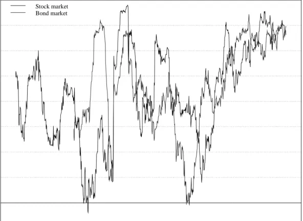
To assess possible time-variation or structural breaks, the correlation is often calculated over either non-overlapping sub-periods or a moving window.7 As an example, moving 52-week correlations between German and US returns on bonds and stocks, respectively, are shown in Figure 1. It demonstrates how strongly moving correlations can change over time. However, the marked ups and downs may only reflect the strong influence of single large price shocks on such “short-memory” correlations. This sensitivity renders a structural interpretation of this measure of international asset price linkages rather doubtful.
7
See, for example, Deutsche Bundesbank (1997), p. 30 f.
Figure 1: Moving cross-country return correlation on stock and bond markets
Germany vs the United States; moving 52-week window
81 82 83 84 85 86 87 88 89 90 91 92 93 94 95 96 97 98 99 -0.1 0.0 0.1 0.2 0.3 0.4 0.5 0.6 0.7 0.8 Stock market Bond market
3.
The methodological framework: ARCH and SWARCH models
In order to measure and model international asset price linkages more reliably, an econometric modelling technique should be applied which takes into account the specific time-series properties of short-run asset returns (and which should be less sensitive to single price shocks). Most importantly, the strong volatility clustering in weekly stock and bond market returns as well as their unconditional non-normality have to be modeled. For this purpose, ARCH-type models (AutoRegressive Conditional Heteroskedasticity) have become a widely applied tool.8 They can be specified very flexibly according to the specific data needs, which has led to the development of a wide variety of types.9 We shall begin with a bivariate AR(1)-GARCH(1,1) specification for each pair of either stock or bond returns. In most cases such a parsimonious specification suffices. First, the near-unpredictability of short-run asset returns allows us to restrict the forecast equations for the conditional means to simple AR(1) processes.10 Second, while the volatility of returns contains substantial predictability, most of its dynamics can usually be captured by a low-order GARCH system.
The AR(1) part describes the conditional means as:
(1) rj,t =µj,t+εj,t with µj,t =Et
[
rj,t Ωt−1]
=αj +βjrj,t−1 for j=asset x,assetywhere rj,t denotes the weekly return of asset j, µj,t for the expected return conditional on information Ωt-1 (in a linear projection), and εj,t a random error. The error vector εt is assumed to follow a bivariate
normal distribution, with zero mean and a time-varying covariance matrix Ht:
(2) εt Ωt−1∼N(0,Ht)
The system is completed by three equations which describe the dynamics of the distinct elements of
Ht. Because of the symmetry of Ht , this subsystem can be summarised with the “vech representation”
of our bivariate GARCH(1,1) model:11
(3) + ε ε ε ε + = − − − − − − − 1 , 1 , 1 , 33 32 31 23 22 21 13 12 11 2 1 , 1 , 1 , 2 1 , 33 32 31 23 22 21 13 12 11 22 12 11 , , , t y t y x t x t y t y t x t x t y t y x t x h h h b b b b b b b b b a a a a a a a a a c c c h h h
with hj,t the conditional error variance of the return of asset j, and hxy,t the conditional covariance. In
this unrestricted system, international “volatility transmission” can occur through a variety of mechanisms. For example, the variance hx,t depends – via the parameters a12, a13, b12and b13 – directly
on the lagged residuals and lagged variance of asset y. Moreover, there is also a mutual contemporaneous dependency which comes through the covariance function hxy,t. In effect, this
function determines the expected comovement between asset returns, although the causal direction of this interrelationship is not identified a priori.12 We can estimate the degree of comovement dimension-free by the time-varying (conditional) correlation coefficient:
8
For a review of the theory and broad empirical evidence, see Bollerslev et al. (1992).
9
See Bollerslev et al. (1992) or Bera and Higgins (1993).
10
See Cochrane (1999), p. 37. The same does not generally hold for long-run returns, which is often partially predictable. For a discussion of this issue and some recent evidence, see, for example, Campbell et al. (1998), Chapter 2, and Domanski and Kremer (1998, 1999).
11
The general form of the vech representation is:
∑ ∑ = − = ε−ε − + + = p j j t j q i i t i t i
t vech C Avech Bvech H
H vech 1 1 ) ( ) ’ ( ) ( ) ( .
The vech operator stacks all elements on and below the main diagonal of an n×n symmetric matrix column by column into an n(n+1)/2-dimensional vector. The coefficient matrices A and B are accordingly of dimension n(n+1)/2×n(n+1)/2).
12
To determine causality, one would have to impose identifying restrictions on the variance covariance matrix which would make the residuals orthogonal as in many structural VAR representations.
(4) ρt = hxy,t/(hx,t hy,t)
0.5
This measure should be superior to the simple correlations as used in Section 2 since it is estimated within a consistent econometric framework. Nevertheless, estimating the full vech representation faces two serious drawbacks. First, positive definiteness of the variance covariance matrix is not guaranteed. Second, the system is heavily overparameterised (bivariate GARCH(1,1) models require 21 coefficients to be estimated for the variance covariance process alone). To mitigate these problems, two restricted representations are applied: first, we impose zero-restrictions on all elements below and above the main diagonal of the coefficient matrices A and B. This “diagonal representation” suggested by Bollerslev et al. (1988) reduces the estimating burden to nine parameters. The conditional variance processes equal those of univariate GARCH models since neither squared lagged residuals nor the lagged variance of one variable appear in the variance equation of the other. Hence, the international volatility transmission can now occur only through the conditional covariance process. The diagonal representation of the bivariate base model (with some convenient changes in notation) looks as follows: (5) + ε ε ε ε + = − − − − − − − 1 , 1 , 1 , 2 1 , 1 , 1 , 2 1 , , , , 0 0 0 0 0 0 0 0 0 0 0 0 t y t y x t x y xy x t y t y t x t x y xy x y xy x t y t y x t x h h h b b b a a a c c c h h h
Second, the model can be further simplified by assuming a constant correlation coefficient ρt = ρ as
proposed by Bollerslev (1990). In this case, the conditional covariance function degenerates to the identity:
(6) hxy,t = ρ (hx,t hy,t)
0.5
Together with the two unchanged conditional variance processes, it forms the “constant correlation representation” which leaves seven parameters to be estimated.13 Positive definiteness of the variance covariance matrix can now be guaranteed. Despite its restrictive nature (it does not permit any lagged international volatility spillovers), the constant correlation representation renders it quite useful. First, it provides a simple summary measure of international asset price linkages, immediately challenging the simple return correlation. Second, it offers an easy way of directly testing specific hypotheses about possible determinants and the structural stability of the correlation coefficient. Concerning its presumed dependence on volatility regimes, the parsimony of the constant correlation representation makes it a natural candidate for multivariate switching-regime ARCH (SWARCH) models which multiply the number of parameters to be estimated.14
However, since multivariate SWARCH models soon become intractable when more than two or three endogenous variables are involved, the present paper confines itself to univariate SWARCH models which are used to identify volatility regimes in certain asset returns. SWARCH models date back to the independent work of Cai (1994) and Hamilton and Susmel (1994). This model class allows conditional volatility to be both time- and state-variant while the volatility regimes are identified and estimated endogenously. The appropriate number of states remains an empirical question and can be tested statistically. We further the hypothesis of two states, i.e. periods of high and low volatility. In the univariate case, the variance equation when allowing for two different states St = 1 or 2 is given
by:15
13
The BEKK representation, as another variant of multivariate GARCH models, works without (a priori) imposing zero-restrictions upon the off-diagonal elements of the matrices A and B. Instead, it uses non-linear cross-equation zero-restrictions to reduce the estimating burden. A recent application to bond rates for the G3 countries is Herwartz and Reimers (1999).
14
Ramchand and Susmel (1998) successfully applied univariate and bivariate SWARCH models to assess regime-dependent cross correlations between weekly stock returns of a broad set of countries.
15
To save degrees of freedom, the AR(1) model for the mean return equation 1 remains state-independent as is the case in related work. This assumption is not very restrictive due to the near-unpredictability of weekly returns.
(7) hS,t =cS +aSεt2−1+bSht−1
t t
t
t for St = 1, 2
This specification follows the “generalised regime switching” (GRS) model of Gray (1996) and differs from the models of Cai and Hamilton and Susmel. The original SWARCH models were restricted to low-order ARCH processes because they assumed that regime-switching GARCH models would be “intractable and impossible to estimate due to the dependence of the conditional variance on the entire past history of the data in a GARCH model”.16 Gray (1996) solved the problem of path dependence by recognising that the conditional density of the endogenous variable is essentially a mixture of distributions with time-varying mixing parameters. If conditional normality is assumed within each regime, the variance at time t can be calculated, in our case very simply, as:
(8) t t t t t t t t t h p h p r E r E h , 2 , 1 , 1 , 1 2 1 1 2 ) 1 ( ] [ ] [ − + = Ω − Ω = − −
where p1,t =Prob
[
St =1Ωt−1]
denotes the conditional probability at time t of being in state 1 given information at time t-1.17 Now ht, which is not path-dependent, can be used as the lagged conditionalvariance in constructing h1,t+1 and h2,t+1 as described in equation 7. However, the main feature of
Markov switching models is the parameterisation of the probability law that causes the unobserved (latent) regime indicator St to switch among regimes.
18,19
In this study, we focus on the simplest case of a two-state, first-order Markov process (where St only depends on the state of the previous period)
with constant “transition probabilities”:
(9) Prob
[
St = jSt−1=i,Ωt−1]
=Prob[
St = jSt−1=i]
= pij for i = 1, 2 and j = 1, 2The probability pi j gives the probability that state i will be followed by state j. However, since the
restriction:
(10) pi1+pi2 =1 for i = 1, 2
applies, only two of these four probabilities can be determined independently. We focus on the regime probabilities p11 and p22 and substitute out the switching probabilities p12 and p21 by using (10). Since the conditional probability p1,t only depends on the regime the process is in at time t-1, it can be expressed as: (11)
[
]
[
] [
]
[
1 1]
22[
1 1]
11 1 1 2 1 1 1 1 2 Prob ) 1 ( 1 Prob Prob , 1 Prob 1 Prob − − − − − − = − − − Ω = − + Ω = = Ω = Ω = = = Ω =∑
t t t t t t i t t t t t S p S p i S i S S SThe Prob
[
St−1=iΩt−1]
can be obtained by updating the probabilities Prob[
St−1=iΩt−2]
using the incoming information rt-1 (since Ωt-1 = {rt-1, Ωt-2} in our case) according to Bayes’ Rule:(12)
[
]
[
]
[
]
[
]
∑
= − − − − − − − − − Ω = Ω = Ω = Ω = = Ω = = Ω = 2 1 2 1 -t 2 1 -t 1 2 1 -t 2 1 -t 1 2 , 1 1 -t 1 1 -t S Prob ) , S ( S Prob ) , S ( S Prob S Prob i t t t t t t t t t i i r f i i r f r i i 16 Gray (1996), p. 34. 17See equation 8 in Gray (1996), p. 34.
18
Markov switching models owe their name to the assumption that St depends upon St-1, St-2, ..., St-r, in which case the
stochastic process of St is named as an r-th order (in general K-state) Markov chain. 19
If the whole path of St is known a priori, the estimation problem would be reduced to that of a simple GARCH model
where: (13) − −α−β π = = = Ω = − − − − − − − 1 , 2 2 1 1 , 1 -t 1 2 1 -t 1 2 ) ( exp 2 1 ) S ( ) , S ( t i t t t i t t t h r r h i r f i r f
is the density of the conditionally normally distributed returns variable rt-1 conditional on a given state
i. Combining (11) and (12) provides a relatively simple non-linear recursive scheme for the “filtered
probability” of regime 1:20 (14) − = + = − = − + − = + = = = − − − − − − − − − − − − − − − − − − ) 1 ( ) 2 ( ) 1 ( ) 1 ( ) 2 ( ) 1 ( ) 1 ( ) 2 ( ) 1 ( ) 1 ( 1 , 1 1 1 1 , 1 1 1 1 , 1 1 1 22 1 , 1 1 1 1 , 1 1 1 1 , 1 1 1 11 , 1 t t t t t t t t t t t t t t t t t t t p S r f p S r f p S r f p p S r f p S r f p S r f p p
The log-likelihood function log L can then be written as:
(15)
∑
[
]
= = − + = = T t t t t t t t f r S p f r S p L 1 , 1 , 1 ( 1) (1 ) ( 2) log logHence, it also possesses a recursive structure similar to the log likelihood of conventional GARCH models. The function can be maximised with respect to p11, p22, α, β, c1, c2, a1, a2, b1, b2 after choosing appropriate starting values.21
All GARCH and SWARCH models in this paper were estimated by maximising the respective log-likelihood functions numerically using the RATS instruction MAXIMIZE with the BFGS algorithm. We always maintained the assumption of normally distributed errors, although in many cases the standardised residuals, while otherwise quite well-behaved, still showed a substantial degree of excess kurtosis. Even under this condition, maximisation of the log-likelihood function should still yield reasonable parameter estimates. This procedure is described as pseudo or quasi-Maximum Likelihood (QML).22 But since the standard errors are likely to be severely biased, we computed them from the heteroskedasticity-consistent variance covariance matrix as proposed by White (1982).
4.
International correlation of asset price movements: does market
turbulence matter?
The empirical analysis starts with an estimation of the constant correlation representation of bivariate AR(1)-GARCH(1,1) models as the most restricted specification. Following this “base model”, we estimate the diagonal representation, which delivers a time-varying correlation coefficient as described in equation 4. This allows us to obtain a first visual impression about the dynamics of international asset price linkages. However, to test hypotheses about the driving factors behind these dynamics, the constant correlation representation is more often used in the literature because of its ease and
20
The literature makes a distinction between “filtered probabilities” and “smoothed probabilities”. The smoothed probabilities use all information available for the entire sample t = 1,...,T to make inferences about the state prevailing at each date t. They are thus more ex post in character. The filtered probabilities, by contrast, use only information up to the respective forecast origin and are therefore more ex ante-oriented. See Kim and Nelson (1999), chapter 4, for details.
21
In fact, to ensure that the estimated transition probabilities p11 and p22 lie in the interval (0, 1), they are constrained by the transformation pii = exp{π ii}/(1+ exp{π ii}). The numerical optimisation is then applied with respect to the unconstrained π ii.
22
tractability. Within the present context, it allows the correlation coefficient to be modelled as a function of different economic states.23 For example, Longin and Solnik (1995) test whether the correlation changes with a priori defined variance regimes (smooth versus turbulent periods) which enter the model as shift dummies in the correlation function. As a methodology that does not rely on a priori defined regimes, we apply parsimonious SWARCH models to identify different volatility states endogenously and to see whether simple return correlations change with the regimes.
4.1 Correlation across major stock markets
Table 2 reports the results of the bivariate GARCH models for each pair of the US, German and Japanese weekly stock returns. There are some general results which hold for each pair of countries irrespective of the model’s representation. As is to be expected, stock returns are materially unpredictable on the basis of the past week’s returns as indicated by the β coefficients, with the result that the constants α in the conditional mean equations roughly equal the respective sample means as shown in Table 1.24 The variance equations all look reasonable and are in line with results generally found in the literature using higher-frequency financial data. The conditional variances are highly persistent as judged by the sum of the autoregressive coefficients (aj + bj), which in all cases never
reaches, but still comes close to, one.25 Most of the persistence derives from the lagged variance rather than the lagged squared residuals, which tends to smooth out the conditional variance process somewhat. The last three lines of Table 2 show the unconditional moments of the variance covariance matrix. The unconditional variances also appear reasonable except for two of the three Japanese equations. In these two cases, the implied steady-state volatilities (with 8.89 and 9.13) seem to be biased upwards when compared with the ordinary sample variance (5.86).26
The correlation coefficients are very precisely estimated with the constant correlation representation. Furthermore, they do not differ much from the unconditional sample moments except in the German-Japanese case, where they are considerably lower. This result changes somewhat under the diagonal representation. The implied unconditional correlation is much higher in the US-German case but lower for both the US-Japanese and the German-Japanese case. However, these results may be overstated since the constants in the three conditional covariance equations – and thus the unconditional moments, too – are rather imprecisely estimated and may therefore contain a substantial bias.
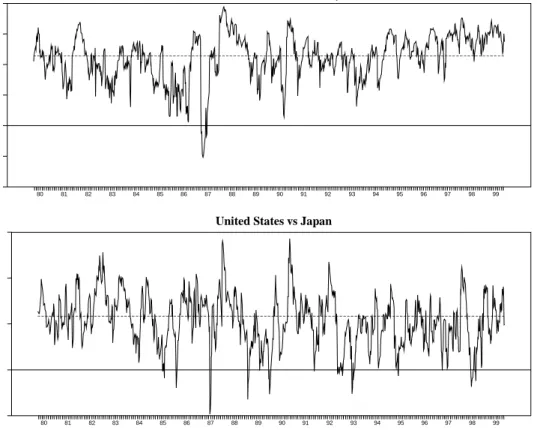
We now turn to the dynamics as implied by the time-varying correlation coefficient from the diagonal GARCH representation as defined in equation 4. Figure 2 shows the time series of this correlation for the US-German case and the US-Japanese case respectively (solid line). The dashed line marks the correlation as estimated by the constant correlation representation. For one thing, the US-Japanese correlation is more variable than the US-German correlation. For another, the first seems to revert rather quickly to its “mean” value over the entire sample, while the latter remains for quite a long time either below or above its supposed attractor level. Furthermore, the visual inspection might suggest that the US-German correlation has been following a moderate upward trend at least since 1993 (or even since 1988). However, we were unable to confirm this hypothesis statistically.27
23
Alternatively, the correlation could also be modelled as a function of deterministic time trends or of any information variable. Recent related studies which have applied this framework are Longin and Solnik (1995) and Bodart and Reding (1999).
24
This picture does not change when estimating first-order VAR(1)-GARCH(1,1) models that add the other country’s lagged return to the explanatory variables.
25
The approximate unit root in the autoregressive polynomial questions the stationarity of the conditional variance process and has led to the development of so-called IGARCH models (integrated in variance). See Bollerslev et al. (1992), p. 14f.
26
The unconditional variance, for example, can be calculated as cj/(1 – aj – bj ) by applying the law of iterated expectations.
See Bera and Higgins (1993), p. 314.
27
We tried deterministic trend variables – beginning in either 1988 or 1993 – as an explanatory variable in a linear function for the correlation coefficient in the constant correlation representation. However, the estimated coefficients were highly insignificant in both cases. We also tested for secular trends in correlation over the whole sample, but this test also failed.
Table 2
Bivariate AR(1)-GARCH(1,1) models for major stock markets
tion representa diagonal (5b) tion representa n correlatio constant ) ( (6) (5a) y) country vs (country x , for (1) 1 , 1 , 1 , , 5 . 0 1 , 1 , , 1 , 2 1 , , , 1 , , − − − − − − − − + ε ε + = ρ = + ε + = = ε + β + α = t xy xy t y t x xy xy t xy t y t x t xy t j j t j j j t j t j t j j j t j h b a c h h h h h b a c h y x j r r
Constant correlation representation Diagonal representation
US vs DE US vs JP DE vs JP US vs DE US vs JP DE vs JP α x 0.267 (0.057) 2 0.297 (0.055)2 0.263 (0.062)2 0.286 (0.058)2 0.303 (0.051)2 0.274 (0.065)2 β x –0.035 (0.031) –0.042 (0.034) 0.044 (0.035) –0.046 (0.032) –0.039 (0.029) 0.049 (0.036) α y 0.249 (0.057) 2 0.249 (0.053)2 0.235 (0.051)2 0.244 (0.047)2 0.245 (0.055)2 0.249 (0.059)2 β y 0.030 (0.030) 0.039 (0.031) 0.043 (0.034) 0.037 (0.028) 0.048 (0.030) 0.031 (0.032) cx 0.245 (0.153) 0.250 (0.229) 0.351 (0.133) 2 0.232 (0.135) 0.208 (0.106)1 0.387 (0.165)1 cy 0.367 (0.115) 2 0.143 (0.062)1 0.130 (0.070) 0.351 (0.156)1 0.155 (0.070)2 0.175 (0.069)1 cxy – – – – – – 0.126 (0.076) 0.104 (0.054) 0.209 (0.123) ax 0.099 (0.041) 1 0.098 (0.056) 0.170 (0.046)2 0.088 (0.036)1 0.087 (0.029)2 0.165 (0.051)2 ay 0.161 (0.038) 2 0.141 (0.030)2 0.136 (0.029)2 0.148 (0.047)1 0.154 (0.028)2 0.133 (0.024)2 axy – – – – – – 0.087 (0.037) 1 0.115 (0.026)2 0.129 (0.051)1 bx 0.845 (0.064) 2 0.845 (0.098)2 0.758 (0.057)2 0.858 (0.053)2 0.865 (0.042)2 0.752 (0.069)2 by 0.761 (0.045) 2 0.842 (0.033)2 0.849 (0.032)2 0.776 (0.066)2 0.829 (0.032)2 0.842 (0.028)2 bxy – – – – – – 0.846 (0.065) 2 0.813 (0.061)2 0.679 (0.148)2 ρ 0.457 (0.019)2 0.352 (0.028)2 0.273 (0.033)2 – – – – – – hx* 4.395 – 4.374 – 4.878 – 4.280 – 4.392 – 4.680 – hy* 4.692 – 8.575 – 8.890 – 4.597 – 9.126 – 6.798 – ρ* – – – – – – 0.578 – 0.227 – 0.194 –
Note: The table gives the estimated coefficients calculated by Maximum Likelihood using the BFGS algorithm. Heteroskedasticity-consistent standard errors in parentheses. Effective sample: 24 January 1980 to 16 September 1999 (1,026 usable observations). 1(2) indicates significance at the 5% (1%) level. hj* is the unconditional variance of country j’s
unexpected return, and ρ* is the unconditional correlation coefficient, both calculated as the steady-state solutions to the variance and covariance equations 5a and 5b and using the definition of the correlation coefficient.
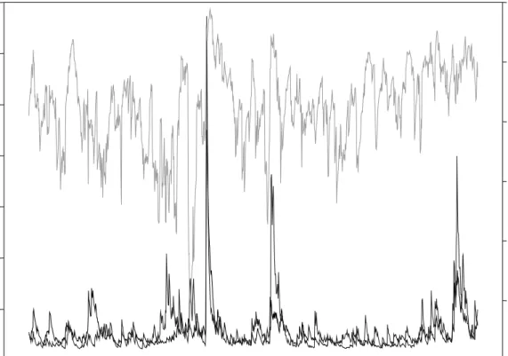
It is often argued that international stock market correlations increase in periods of stress with high conditional return volatilities. Figure A1 in the Appendix gives a visual impression of why this hypothesis is raised so often. The conditional variance series for both the United States and Germany are shown in the lower part, while the corresponding correlation coefficient appears in the upper part. Obviously, the correlation jumps upwards when both markets are hit by large shocks, as in October 1987 and August 1990. Empirical evidence in favour of this hypothesis is provided, for instance, by Koch and Koch (1991), and Longin and Solnik (1995). However, these studies did not find a statistically fully convincing solution to the problem of separating volatility regimes. Lacking a proper methodology, they had to define the sub-periods of high versus low volatilities exogenously in an ad hoc fashion. SWARCH models now provide a technology for doing this job endogenously. They were first applied in this context by Ramchand and Susmel (1998), who find strong evidence for state-dependent correlations across weekly stock returns for a large set of countries.
This result does not necessarily contradict the findings in Longin and Solnik (1995), who used a much larger sample (1960 to 1990) with monthly stock returns for their bivariate GARCH models.
Table 3 presents our results of univariate SWARCH specifications. The model produces similar estimates for all of the stock returns. Most noticeable are the clear-cut and highly significant differences in the two identified, country-specific variance regimes.28 The unconditional variances of the high volatility state are three to five times larger than those of the low volatility state. Moreover, the use of the generalised regime-switching model specification of Gray (1996) proves to be advantageous since it allows the persistence parameter aSt to differ between regimes in contrast to the
original SWARCH specifications. Within the low volatility state, the variances remain virtually constant due to the negligible (and insignificant) autoregression coefficients a1. In the high volatility state, however, lagged squared residuals do have a significant and materially important influence on current conditional variances via parameters a2. This makes large initial shocks, as typically observed
in market crashes, persist for some time.
Furthermore, each regime itself is highly persistent as evidenced by the large (and, in general, highly significant) constant regime probabilities p11 and p22, respectively.29 This result is consistent with applications of Markov switching in many other contexts. Accordingly, the time series for the conditional regime probabilities look quite reasonable. As an example, Figure 3 presents the conditional probability of German stock returns being in state 1 (p1,t), the low variance regime. This
28
We have to admit that individual standard errors of the parameters of the state-dependent variance equations do only provide an informal test of the two-state model against a simple one-state specification, since under the null hypothesis of no-regime switching the parameters of the second state’s variance equation are not identified. However, we regard the evidence in favour of the two-state model as so strong that we dispensed with a proper non-standard test such as that developed by Hansen (1992).
29
Table 3 does not show standard errors for the “constrained” transition probabilities since standard errors were only obtained for the unconstrained probability parameters which are not directly interpretable and thus not shown in the table.
Figure 2: International stock return correlations from bivariate GARCH models
Constant correlation representation (dashed) and diagonal representation (solid)
United States vs Germany
80 81 82 83 84 85 86 87 88 89 90 91 92 93 94 95 96 97 98 99 -0.4 -0.2 0.0 0.2 0.4 0.6 0.8
United States vs Japan
80 81 82 83 84 85 86 87 88 89 90 91 92 93 94 95 96 97 98 99 -0.30 0.00 0.30 0.60 0.90
probability is (i) either near one or close to zero, and this (ii) for extended periods of time. The second quality reflects the high regime (or low transition) probabilities. The first property indicates the good performance of the conditional probability in classifying volatility regimes since, being close to its boundaries, it provides a clear signal as to whether a given observation belongs to a certain regime or not. This quality can be measured statistically by the Regime Classification Measure (RCM) proposed by Ang and Bekaert (1998). The RCMs for the SWARCH models of German, Japanese and US returns lie between 35 and 55 (see Table 3). Being so low, the RCMs prove our visual impression that the regime inference of the SWARCH models is generally strong and, hence, quite reliable.30
Table 3
Univariate SWARCH(2,1) models for major stock markets
[
S S]
for 1,2in thiscaseProb (9) 2 , 1 for (7) (1) 1 -t t 2 1 , 1 = = = = = = ε + = ε + β + α = − − j i i j p S a c h r r j i t t S S t S t t t t t t
United States Germany Japan
Parameter Estimate Std. Error Estimate Std. error Estimate Std. error
α 0.304 (0.061)2 0.244 (0.097) 1 0.169 (0.060)2 β –0.037 (0.034) 0.021 (0.038) 0.063 (0.038) c1 2.249 (0.281)2 2.301 (0.354)2 2.148 (0.284)2 c2 7.146 (1.747)2 7.326 (2.562)2 9.785 (1.409)2 a1 0.039 (0.058) 0.005 (0.035) 0.032 (0.064) a2 0.173 (0.158) 0.226 (0.091)1 0.151 (0.060)1 p11 0.973 – 0.991 – 0.982 – p22 0.939 – 0.985 – 0.972 – h1* 2.339 – 2.312 – 2.220 – h2* 8.644 – 9.469 – 11.521 – ARCH(4) 0.75 (0.55) 1.70 (0.15) 2.27 (0.06) RCM 55.7 34.9 40.9
Note: The table gives the estimated coefficients calculated by Maximum Likelihood using the BFGS algorithm. Heteroskedasticity-consistent standard errors in parentheses. – ARCH(4) is an F-test statistic for the null hypothesis of no ARCH effects in standardised residuals up to lag 4 with p-values in brackets. – RCM is the regime classification measure as proposed by Ang and Bekaert (1998) which lies between 0 (perfect classification) and 100 (no information). Effective sample: 31 January 1980 to 16 September 1999 (1,025 usable observations). 1(2) indicates significance at the 5% (1%) level. h1* is the unconditional variance in the low volatility state, and h2* is the unconditional variance in the high volatility state. They are calculated as the steady-state solutions to each state’s variance equation, i.e.: * /(1 )
t t t S S S c a h = − for St = 1, 2.
Also note that we specified the variance processes without a GARCH term. We can dispense with lagged conditional variances since they proved to be insignificant in all cases. This fact is consistent with the presumption that the near-unit root in the conditional variance process of conventional GARCH models (as mentioned above) does not reflect “true” volatility persistence, but instead results
30
Ang and Bekaert (1998), p. 15, define the RCM statistic (here for two states) as:
∑
= − ⋅ = T t t t p p T RCM 1 , 1 , 1 (1 ) 1 400 . In a
perfectly classifying regime-switching model the conditional probability would always be infinitesimally close to 1 or 0, keeping the RCM at value 0. On the other hand, if the probabilities hover around 0.5, the model would provide no regime information, boosting the RCM to 100. The fact that the RCM for the German model is indeed rather low can be judged from the average product of regime probabilities RCM/400 = 0.087. It implies that the dominating regime probability on average equals 0.903, which is rather high.
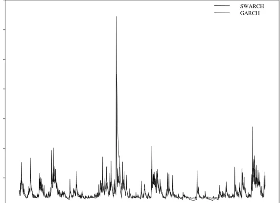
as a bias from the neglect of structural breaks such as different variance regimes.31 The fact that we can actually take out the GARCH terms without rendering the SWARCH model less powerful may be seen from Figure 4, which compares the conditional variance process for US stock returns of the SWARCH model with that of a GARCH model.32 The conditional variance of the SWARCH model is calculated according to equations 7 and 8, i.e. the variance processes of each state are weighted by their time-varying conditional regime probability. The degree of overlap between the two time series is impressive, so that even a parsimonious SWARCH specification is able to generate rich volatility dynamics stemming from the non-linearities implied by Markov switching variance regimes.
We are now in a position to calculate regime-dependent cross correlations, as is done by Ramchand and Susmel (1998). The low variance and high variance states in each market were identified using the classification system of Hamilton (1989), wherein an observation belongs to state 1 or 2 whichever state’s conditional probability pi,t =Prob
[
St =iΩt−1]
is higher than 0.5.33 Under this assumption, four possible states have to be considered in a bivariate setting. For instance, if we want to correlate US and German stock returns, the following four states emerge:3431
Lamoureux and Lastrapes (1990) studied this point in more depth.
32
The GARCH process is taken from the bivariate US-German model in the constant correlation representation as given in Table 2, but any other estimated GARCH model for US returns produces almost identical results.
33
While Hamilton proposes the smoothed probabilities for defining regimes, we shall use the filtered probabilities instead, because they are also used for the calculation of the conditional variance process and owing to their ex ante nature.
34
Instead of estimating bivariate four-state SWARCH models, this paper focuses on separately calculated simple correlation coefficients for each of the four states. First, unrestricted four-state SWARCH models are difficult to estimate. The transition matrix alone contains 12 transition probabilities to be estimated without further restrictions. Second, the
Figure 3: Conditional probability of being in the low variance regime
From a SWARCH model of German stock returns
80 81 82 83 84 85 86 87 88 89 90 91 92 93 94 95 96 97 98 99 0.00 0.25 0.50 0.75 1.00
St = 1: US variance low, German variance low
St = 2: US variance low, German variance high
St = 3: US variance high, German variance low
St = 4: US variance high, German variance high
35
The results of the return correlations across these four states are given in Table 4.36 They confirm the general hypothesis of correlations increasing along with volatility. Hence, “market turbulence matters” indeed. For example, the US-German correlation increases to 0.63 when both countries experience high volatilities (state 4) compared with 0.40 in the case of low volatilities (state 1). The same pattern holds for the remaining country pairs. The intermediate states suggest the following interpretation: the US market seems to dictate the degree of international stock price synchronisation. If US returns are in the high volatility state, the correlation with German and Japanese returns is also high, regardless of whether foreign returns belong to the high or to the low volatility state. Conversely, if US returns are in the low volatility state, the correlation with foreign returns also diminishes. Furthermore, the correlation between German and Japanese returns is minor except when both returns become more
two-step, “system-free” procedure provides a tractable way of obtaining state-dependent correlations even when a larger set of countries or asset classes is considered. However, this entails the disadvantage of not obtaining an independent estimate of the conditional regime probabilities which could be used for forecasting purposes.
35
Comparing the conditional variance series of different countries suggests that the distinction between four states does make sense. Figure 3, for example, shows volatility hikes in Germany which occur independently of volatility movements in the United States, and vice versa. Thus, volatility cycles are generally not fully synchronised, which argues against the general validity of the contagion hypothesis.
36
We also calculated the correlations between the residuals from the SWARCH models instead of total returns, but the results were absolutely unchanged to the first and second decimal place.
Figure 4: Conditional variance from a SWARCH and GARCH model
US stock returns 80 81 82 83 84 85 86 87 88 89 90 91 92 93 94 95 96 97 98 99 0 8 16 24 32 40 48 56 SWARCH GARCH
volatile at the same time. This may again be the result of a common dependency on US returns. It is also worth mentioning that each state for each pair of countries occurs sufficiently often to enable a reasonable estimate of the corresponding correlation coefficient to be obtained, although tranquil periods are more frequent than turbulent ones.
Table 4
Stock market cross correlation in different volatility regimes
Correlation Observations United States vs Germany
State 1: US low, Germany low 0.40 601
State 2: US low, Germany high 0.44 185
State 3: US high, Germany low 0.61 88
State 4: US high, Germany high 0.66 151
United States vs Japan
State 1: US low, Japan low 0.30 542
State 2: US low, Japan high 0.27 244
State 3: US high, Japan low 0.44 102
State 4: US high, Japan high 0.59 137
Germany vs Japan
State 1: Germany low, Japan low 0.24 531
State 2: Germany low, Japan high 0.23 158
State 3: Germany high, Japan low 0.21 113
State 4: Germany high, Japan high 0.42 223
Note: State classification according to the conditional regime probabilities derived from univariate SWARCH(2,1) models for weekly stock returns. Total sample: 31 January 1980 to 16 September 1999 (1,025 usable observations).
4.2 Correlation across major bond markets
Table 5 presents the estimated coefficients of the bivariate GARCH models for each pair of US, German and Japanese bond returns. Essentially, the models yield the expected results. First, bond returns are lower and less volatile than stock returns, which is properly reflected in the estimated unconditional means and variances. Second, although not economically significant, bond returns contain some predictable elements, as is evidenced by the statistical significance of seven out of 12 autoregressive coefficients in the mean equations. Third, the conditional variance equations look quite familiar, like their stock market counterparts. However, this holds only for the constant correlation representation. The diagonal representation delivers some awkward-looking conditional covariance equations for the bivariate models of Japanese returns, which makes us less confident in this specification.37 Instead, the time-varying correlation between US and German returns follows rather smooth and extended cycles around its steady state (see Figure A2 in the Appendix). Moreover, there exists no discernible time trend in the coefficient, suggesting a structural break with higher correlation in the recent past. Overall, the GARCH models prove again that the short-term linkage between German and US returns is much higher and, at the same time, more stable than the correlation of either of these countries with Japanese bond returns.
37
The structure of these covariance equations implies that the time series of covariances and, hence, the correlation coefficients regularly jump up and down around their medium-term trend. This behaviour is economically unconvincing and leads to the rejection of this specification. Technically speaking, it results from the fact that bond prices in Japan quite frequently do move in the opposite direction to US or German prices, but not for long enough; in turn, this may be caused economically by asymmetric market conditions such as monetary and fiscal policy shocks.
Table 5
Bivariate AR(1)-GARCH(1,1) models for major bond markets
tion representa diagonal (5b) tion representa n correlatio constant ) ( (6) (5a) y) country vs (country x , for (1) 1 , 1 , 1 , , 5 . 0 1 , 1 , , 1 , 2 1 , , , 1 , , − − − − − − − − + ε ε + = ρ = + ε + = = ε + β + α = t xy xy t y t x xy xy t xy t y t x t xy t j j t j j j t j t j t j j j t j h b a c h h h h h b a c h y x j r r
Constant correlation representation Diagonal representation
US vs DE US vs JP DE vs JP US vs DE US vs JP DE vs JP α x 0.047 (0.038) 0.038 (0.035) 0.051 (0.021) 1 0.046 (0.031) 0.042 (0.031) 0.049 (0.022)1 β x –0.038 (0.031) –0.016 (0.038) 0.077 (0.039) 1 –0.046 (0.039) –0.019 (0.033) 0.081 (0.027)2 α y 0.047 (0.025) 0.067 (0.031) 1 0.073 (0.026)2 0.044 (0.026) 0.068 (0.024)2 0.074 (0.025)2 β y 0.077 (0.034) 1 0.086 (0.037)1 0.090 (0.036)1 0.069 (0.039) 0.091 (0.039)1 0.095 (0.044)1 cx 0.087 (0.035) 1 0.075 (0.043) 0.019 (0.007)2 0.080 (0.033)1 0.074 (0.035)2 0.022 (0.007)2 cy 0.028 (0.011) 1 0.076 (0.023)2 0.075 (0.021)2 0.033 (0.016)1 0.074 (0.020)2 0.080 (0.022)2 cxy – – – – – – 0.018 (0.006) 2 0.296 (0.052)2 0.225 (0.051)2 ax 0.078 (0.028) 2 0.072 (0.024)2 0.114 (0.027)2 0.079 (0.025)2 0.072 (0.022)2 0.108 (0.022)2 ay 0.116 (0.031) 2 0.143 (0.037)2 0.135 (0.036)2 0.105 (0.032)2 0.139 (0.033)2 0.126 (0.034)2 axy – – – – – – 0.053 (0.011) 2 –0.026 (0.021)2 –0.034 (0.026)2 bx 0.839 (0.047) 2 0.856 (0.054)2 0.855 (0.026)2 0.844 (0.043)2 0.857 (0.045)2 0.853 (0.024)2 by 0.832 (0.040) 2 0.756 (0.054)2 0.763 (0.047)2 0.831 (0.055)2 0.762 (0.042)2 0.763 (0.049)2 bxy – – – – – – 0.893 (0.016) 2 –0.805 (0.121)2 –0.627 (0.240)2 ρ 0.472 (0.026)2 0.215 (0.036)2 0.267 (0.032)2 – – – – – – hx* 1.040 – 1.042 – 0.624 – 1.040 – 1.041 – 0.580 – hy* 0.549 – 0.745 – 0.733 – 0.523 – 0.744 – 0.719 – ρ* – – – – – – 0.451 – 0.183 – 0.210 –
Note: The table gives the estimated coefficients calculated by Maximum Likelihood using the BFGS algorithm. Heteroskedasticity-consistent standard errors in parentheses. Effective sample: 26 January 1984 to 16 September 1999 (817 usable observations). 1(2) indicates significance at the 5% (1%) level. h
j* is the unconditional variance of country j’s
unexpected return, and ρ* is the unconditional correlation coefficient, both calculated as the steady-state solutions to the variance and covariance equations 5a and 5b and using the definition of the correlation coefficient.
In testing for regime dependency of bond market correlation, our two-state SWARCH model failed to identify different volatility regimes in the US case.38 We therefore have recourse to the “threshold” approach, where an exogonenously defined threshold value separates high from low volatility observations.39 Accordingly, an observation belongs to the high (low) volatility regime when squared returns are higher (lower) than the threshold value. While in most cases the threshold is set to the sample standard deviation, we apply different scaling parameters to the unconditional standard deviation in order to mitigate the problem of ad-hocery. The corresponding regime-dependent cross correlations are presented in Table 6. Again, the results strongly confirm the positive relation between market turbulence and international correlation. For example, irrespective of the scaling parameter, the US-German correlation more than doubles when both countries move together from a low volatility to a high variance state. In the US-Japanese case, correlation even increases about five times on average, although it never reaches the absolute values of the US-German linkage. The mixed states 2 and 3 only matter for the relationship between US and German bond returns. The correlation is higher than in the
38
For Germany and Japan, instead, we obtained reasonable results.
39
“low-low state” and almost identical, regardless of whether prices move more in the United States or in Germany. This pattern suggests that larger price movements in one market, which may result from pure idiosyncratic shocks (such as monetary policy shocks), do always spill over to the other market to some degree and thus tighten the measured linkage significantly, without necessarily “exporting” the underlying market uncertainty. Experience suggests that this typically occurs when a market is said to “decouple” from the other, with relative interest rates gradually adjusting to asymmetric outlooks for their fundamental factors while both rates still move synchronously.40
Table 6
Bond market cross correlation in different volatility regimes
η = 0.75 η = 1.00 η = 1.50 Corr. Nobs. Corr. Nobs. Corr. Nobs.
0.25 331 0.28 468 0.33 648 0.35 153 0.47 123 0.65 69 0.37 179 0.49 140 0.60 73 0.71 154 0.79 86 0.83 27 0.10 356 0.10 483 0.12 653 0.09 128 0.10 108 0.38 64 0.13 217 0.25 167 0.24 80 0.44 116 0.54 59 0.62 20 0.12 379 0.10 504 0.17 659 0.11 131 0.42 104 0.44 62 0.12 194 0.28 146 0.22 74
United States vs Germany State 1: US low, Germany low State 2: US low, Germany high State 3: US high, Germany low State 4: US high, Germany high United States vs Japan
State 1: US low, Japan low State 2: US low, Japan high State 3: US high, Japan low State 4: US high, Japan high Germany vs Japan
State 1: Germany low, Japan low State 2: Germany low, Japan high State 3: Germany high, Japan low
State 4: Germany high, Japan high 0.53 113 0.55 63 0.71 22
Note: “Corr.” And “Nobs.” stand for “correlation coefficient” and “number of observations”, respectively. State classification according to an exogenous threshold based on the unconditional standard deviation σ of weekly stock returns rt scaled by the parameter η:
low volatility state, if | rj, t | <η⋅σj
high volatility state, if | rj, t | ≥η⋅σj .
Assuming normally distributed returns, η-values of 0.75, 1.00 and 1.50 predict that approximately 45%, 30% and 13% of absolute returns lie above the threshold, respectively. Total sample: 26 January 1984 to 16 September 1999 (817 usable observations).
Before turning to the empirical results for different German market segments, we have to add a few words of caution, however. As recent studies have demonstrated, even substantial increases in correlation during market turbulence must not be interpreted per se as conclusive evidence of contagion opposed to normal interdependence.41 In fact, the sample correlation should always increase (decrease) relative to its constant population moment when the sampling variance of linearly dependent return variables exceeds (falls below) its “true” unconditional variance (see equation 1 and the corresponding theorem in Loretan and English (1999, this volume)). Hence, upward jumps in asset return correlations in periods of high volatility are to be expected even if the true unconditional correlation – which measures normal interdependence – remains unchanged. The presumed
40
How level linkages (“convergence”) and comovements (“synchronisation”) can be estimated separately within a single empirical framework is shown by Kremer (1999).
41
breakdown in measured correlation may therefore result from such normal interdependence rather than from contagion accompanied by a shift in the unconditional distribution of asset returns.42
How should our results be interpreted in the light of this sampling-bias argument? As a kind of robustness check, we calculated “theoretical” or “expected” correlations between US and German or US and Japanese stock returns according to Loretan and English’s equation 1 under the assumptions that, first, the variance of US returns in the low volatility regime equals the unconditional variance and, second, that volatility regimes are fully synchronised in all countries so that only two states can occur. In the US-German case, the increase in the variance of US returns over high volatility periods justifies an increase in the correlation from 0.41 in tranquil times to 0.58 in turbulent times. The last value comes very close to the measured correlation in the high volatility regime of 0.60. In the US-Japanese case, by contrast, the expected correlation only increases from 0.28 to 0.41, which is substantially lower than the measured correlation of 0.55 in the high volatility state.
This mixed evidence implies some ambiguity in the interpretation of our results, i.e. it remains an open question whether observable changes in stock or bond market correlations result from contagion or merely reflect normal but strong international market linkages. Both hypotheses are observationally equivalent. However, we wish to mention one argument which favours the contagion hypothesis. Regime-switching models actually try to identify shifts in the underlying asset return distributions which may result from significant differences in market participants’ behaviour during periods of stress. Since we have found strong evidence that variance regimes switch over time, it is also plausible to allow unconditional (“structural”) cross-market correlations to switch with changes in the variance regimes.
5.
Spreading of international volatility spillovers through the national
financial markets: do market segments matter?
Volatility spillovers measured on the basis of benchmark segments, such as the yield of 10-year government bonds, do not necessarily reflect the situation in the market as a whole. Instead, a certain decoupling of particular segments of national markets may occur in the wake of international volatility spillovers. If asset price movements in a very general sense are interpreted as the result of information processing, several reasons may be put forward for such a market segmentation: first, the information relevant for price formation may differ between market segments; second, even if the information basis is the same, the processing of information might differ systematically according to the different groups of investors which are most active in the respective markets; third, even if information input and processing are congruent over market segments, the price effect may deviate owing to differing transaction costs or market liquidity.
In order to test the “market segmentation” hypothesis, we calculate return correlations over different volatility regimes between each German stock and bond market segment and the corresponding US benchmark market. The selection of national market segments is based on the presumption that they differ with respect to the set of price-relevant information, the dominant market participants and market liquidity from the 10-year government benchmark bond and the value-weighted DS German equity index, respectively. If the structural differences really matter, they should show up in different international correlation patterns. Table 7 summarises some structural features of the German market segments. In the stock market, the blue chip DAX segment is by far the most liquid and presumably also the most international one. In contrast to this, the medium-sized companies represented in the MDAX as well as the small SMAX shares are far less actively traded. Additionally, different information sets might be relevant for each market if one supposes that MDAX and SMAX companies are less international (in terms of business activity) than those in the DAX.
42
Actually, the empirical results presented in Forbes and Rigobon (1999) as well as Loretan and English (1999, this volume) argue against the contagion hypothesis.
Table 7
Features of German securities markets
Market segment Market capitalisation
(euro bn)
Number of issues
Average market value per issue outstanding
(euro bn) Futures contracts traded Turnover/ market capitalisation1 Foreign participation2 Stock market
DS Germany 965.4 no derivative n.a. n.a.
DAX 791.2 30 26.4 1.0883 0.68 n.a.
MDAX 116.7 70 1.7 743 0.24 n.a.
SMAX 19.9 107 0.2 no derivative 0.29 n.a.
Bond market
Bund 10-yr 54.1 4 13.5 99.0934 n.a.
Bund 7-yr 22.5 2 11.3 no derivative n.a.
Bund 5-yr 47.6 7 6.8 32.5094 n.a.
130%
Bund 2-yr 50.6 8 6.3 10.9784 n.a. 75%
Pfandbriefe 10-yr 177.3 2.94 0.1 no derivative n.a. 30%
Note: Figures are as of August 1999 or as indicated. 1
Average monthly turnover from September 1998 to August 1999 divided by market capitalisation as of end-August 1999. 2 Cumulated net purchases by foreigners from January 1994 to June 1999 related to total net issues. 3 In billions of euros. 4
Number of contracts traded from January 1999 to August 1999 in thousands. Sources: Deutsche Börse; Deutsche Bundesbank; Eurex Germany; own calculations.
For the bond market, the 10-year government bond segment is clearly the most liquid one (as is indicated by the average size of issues and the availability of one of the most actively traded futures contracts worldwide as a hedging instrument) and also the most “international” one. (The available statistics do not allow for a separation of ownership for individual issues. However, anecdotal evidence suggests that international participation – and particularly short-term position-taking – is concentrated in this segment.) The five- and two-year maturities can also be assessed as very liquid and “international”, although less so than the 10-year segment. A stark contrast exists between the structure of the 10-year bund and bank bond segment. The latter is relatively scattered and international participation is only a fraction of that of the bund market (the picture would be different for the liquid Jumbo Pfandbriefe; however, it is not possible to separate them statistically). Compared with the stock market, the information relevant for bond prices could mainly depend on the maturity of the instrument (giving domestic monetary policy a particularly strong and more direct impact at the short end of the yield curve).
5.1 Stock market
The correlation of stock returns between the US market and the different segments of the German market supports the presumption sketched out above that less liquid and less international market segments may be less prone to international turbulence (see Table 8). The correlation pattern between the US market and the DAX is again (see Table 1) very similar to that of the DS index due to the dominance of the blue chips in the latter. The correlation increases by about 50% if both markets switch from a low volatility regime to a high volatility regime at the same time. By contrast, the correlation of MDAX and SMAX shares with the US stock market is significantly lower than that of the DAX if market conditions are calm in Germany. However, all German markets exhibit a similar comovement with US stock prices if Germany is in a high volatility regime. But, in both cases, MDAX and SMAX correlation is broadly unaffected by a switch in the volatility regime in the United States.
Table 8
Cross correlation with the US stock market for different market segments in Germany over different volatility regimes
Correlation with DS United States: German market segment
Volatility regime DS Germany DAX MDAX SMAX
Germany low US low (364) 0.46 0.44 0.39 0.28 US high (13) 0.51 0.54 0.31 0.26 Germany high US low (99) 0.58 0.54 0.54 0.53 US high (94) 0.65 0.65 0.54 0.55
Note: Volatility regimes identified by univariate SWARCH(2,1) models for US and German total market returns (DS indices). Effective sample: 21 October 1988 to 16 September 1999. Number of regime observations in parentheses.
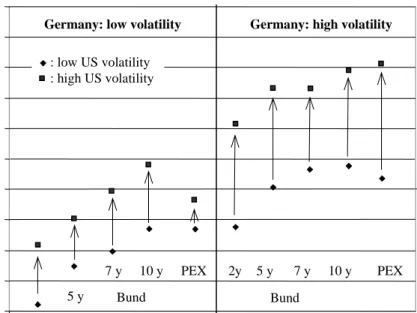
5.2 Bond market
For the bond market, the level of return correlations under different volatility regimes and the impact of a volatility regime shift in the US bond market on the various German market segments support the view that market segments matter (see Figure 5). If both the domestic and the US market are in a low volatility regime, correlation is generally low but increases with longer maturities of German government bonds. This correlation pattern may simply be explained by the fact that the substitutability of 10-year US government bonds and German bonds decreases with shorter maturities
of the latter. From the viewpoint of the information contained in bond prices, this may be a reflection of cyclical differences in domestic factors – namely monetary policies – becoming less important with
0,1 0,2 0,3 0,4 0,5 0,6 0,7 0,8 0,9 PEX PEX Bund 10 y 7 y 5 y 2y Bund 10 y 7 y 5 y 2y
Figure 5: Volatility regime shifts in the US bond market and their impact on the correlation with the German bond market*
*Correlation of weekly returns on 10- year US government bonds and the return in the respective German market segment. Volatility regimes identified by exogenous threshold for unconditional standard deviation (UStd) with low variance regime: |r(t)| < 1.0*UStd, and high variance regime: |r(t) | > 1.0*UStd.
Germany: low volatility Germany: high volatility
: low US volatility : high US volatility
increasing maturities relative to long-term expectations about growth and inflation. The correlation between the highly liquid 10-year bunds and the less liquid Pfandbriefe, on the one hand, and US bonds, on the other, differs only slightly. This may be seen as an indication that arbitrage between both domestic market segments works well during calm periods. A reason for this could be that market liquidity plays a minor role in calm periods.
This picture changes during episodes of high volatility: if the US market switches to a high volatility regime (while Germany remains in the low volatility state), correlation between German government bonds and US Treasuries almost doubles, irrespective of the maturity of the former. The Pfandbrief segment, in contrast, exhibits only a slightly higher correlation. An explanation for this phenomenon might be that the German government bond market, as the most liquid and international segment, is directly affected by the reallocation of international bond portfolios induced by the US market. The Pfandbrief segment might remain relatively unaffected by these transactions because domestic portfolios do not need to be reallocated against a background of still-low domestic volatility. This view changes dramatically if the domestic market switches to a high volatility regime, too. In this case, the correlation between the Pfandbriefe and US Treasuries jumps to 0.81, about the level of the bunds’ correlation.
6.
Conclusion and outlook
The purpose of this paper is twofold. First, we suggest GARCH techniques to measure international asset price linkages when higher-frequency data are used. The proposed measure is either a constant or a time-varying correlation coefficient of (unexpected) weekly asset returns. Second, we investigate whether correlations between German and US bond and stock returns depend on different volatility regimes and, moreover, whether they vary across benchmark products and minor market segments in Germany. The results generally support the view that both the volatility regime and the market structure are important for the strength of international price linkages. Given these results, two questions arise: first, “How can the empirical evidence presented in this paper be interpreted and explained economically?”, and second, “What are the policy implications at the micro and the macro level?”.
GARCH models are essentially descriptive in nature. As in most applications, the models employed here were not derived from first economic principles and thus lack a straightforward theoretical interpretation. Consequently, the theory behind the model has to be superimposed a posteriori. Furthermore, the forces that drive short-term asset prices are modelled as “latent” and hence unobservable variables. Both issues leave a wide range of options among competing theories for the model’s interpretation. Unless the theory imposes a certain structure on the model which leads to testable restrictions, this choice will always be ad hoc and somewhat arbitrary.
A very general approach to interpretation is to view asset price movements as the result of an information-processing activity, comprising the arrival of new information, its analysis by market participants and the interplay of market transactions carried out on the basis of this new information. In this perspective, ARCH effects in high-frequency data can be seen as a manifestation of serial correlation or “time dependence” in the amount of information or the quality of information arriving to the market per period of time, i.e. short-term asset returns are driven by the amount or quality of news reaching the market in clusters.43 This view can be broadened to include the time it takes market participants to assess the information fully (information-processing hypothesis) and the price dynamics created by the responses of market agents to news. For example, traders with heterogeneous
43
For different interpretations of ARCH models, see Bera and Higgins (1993), pp. 322-30, and Bollerslev et al. (1992), p. 40f.
prior beliefs and private information may need some time for information processing and trading – after news has come in – to resolve the expectational differences.44
This framework is able to explain volatility clustering, but not necessarily the closer international comovement of assets prices – i.e. contagion – in turbulent periods. To explain this fact, one has to make assumptions about the nature of shocks behind asset price movements in each market. For example, the study by Engle et al. (1990) suggests that the volatility of short-term asset prices derives mostly from common and hence “international” shocks (“meteor showers”) and less from changes in country-specific fundamentals (“heat waves”). Adopting this framework, we could argue that, first, more tranquil periods are dominated by independent country-specific shocks. The independence assumption implies that international price correlation tends to be lower in such per