MODEL MIXING FOR LONG-TERM
EXTRAPOLATION
Pavel Ettler
1, Miroslav K´arn´y
2, Petr Nedoma
2 1COMPUREG Plzeˇn, s.r.o.
306 34 Plzeˇn, Czech Republic
2
Institute of Information Theory and Automation (UTIA)
182 02 Praha, Czech Republic
[email protected] (Pavel Ettler)
Abstract
Reliable extrapolation – simulation or prediction – of system output is an invaluable departure
point for the control system design. For application of model-based techniques, the
knowl-edge of the model structure is essential. It can be based purely on the physical point of view
or estimated from process data while the system is considered as a black box. Mixing of both
methods results in grey box modelling. Often, modelled systems are governed by several known
physical laws and each of these laws implies a model, which should match the data.
Neverthe-less inevitable uncertainties often make simulated outputs of respective models unreliable. The
problem is especially pronounced for systems with a significant time delay. This motivates
search for methods, which utilize all available models at once and mix their outputs with the
aim to get better results. In the paper, four variants of mixing are considered, discussed and
their performance compared on industrial data. Seeming alternative – a simple complex model
is discussed as well. Data for experiments came from a cold rolling mill.
Keywords: Simulation, modelling, estimation, multiple models.
Presenting Author’s Biography
Pavel Ettler received the doctor degree in cybernetics from the University
of West Bohemia in Plzeˇn. He worked as researcher at ˇSkoda (Rolling
Mills branch) for eleven years. In 1993 he joined COMPUREG, a company
oriented to industrial control systems. His interests include identification
and control of systems subject to uncertainties with application to metal
processing and machine control. His involvement with research includes
participation in several international and national research projects, mainly
in co-operation with UTIA.
1
Introduction
Having data from a real system at disposal, construc-tion of a linear model that extrapolates measured data seems to be simple. The construction relies on the fol-lowing key steps: i) determine the sampling period; ii) choose the maximal model order respecting the dy-namic properties of the system; iii) create the regression vector containing all available explanatory data (regres-sors); and iv) estimate model parameters, typically by least squares [1, 2]. Unfortunately, this purely “black box” modelling often fails in practice due to unknown correlation of data channels, imperfect measurements, unmeasurable disturbances, etc. Moreover, the gained models are usually over-parameterized and unsuitable for simulation or multi-step prediction. Thus, at least rough respecting of known physical relations seems un-avoidable in model building.
Many real systems behave according to several known physical laws. A simple model based on a particu-lar law could be sufficient providing the available data are uncorrupted and informative enough. This case is, however, rare. The systematic grey-box model build-ing [3] is to be used whenever possible to counteract this problem. Often, however, the complexity of the resulting model is too high. Under this situation, ad-dressed here, it is necessary to utilize all available sim-ple models, each representing a particular anticipated relation among data. The particular model outputs are then combined into the overall model output. The paper inspects promising combination possibilities and tests them on real data. They are related to rolling mills [4, 5]. The tested case is exceptional by an inherent significant transport delay and high demands on extrap-olation quality.
All considered models ιM,ι∈ι∗≡ {1,2, . . . ,˚ι}, of a
systemShave the form: ιM: y t= ιθιψ ′ t+ ιξ t, (1)
whereιlabels the model;tstands for the discrete time;
yt denotes system output; ιθ is a vector of unknown regression coefficients; ιψtis the regression vector; and ιξ
tdenotes the zero mean white noise. Often, the noise can be assumed to be normal with a constant variance
rι. Then, the outputytis equivalently described by the normalNyt(·,·)probability density function (pdf)
f(yt|ιψ
t,ιΘ) =Nyt(
ιθιψ′
t, rι),
ιΘ≡(ιθ, rι). (2)
Parameters ιΘ are estimated recursively using data measured on the system. Estimates ιθbof parameters ιθ serve for extrapolation of the output course. They provide output predictions ι
b
yt
ι
b
yt= ιθbt−kιψt′. (3) The subscriptt−kat ιθbt−kstresses that the estimates are based on data recordsd1:t−k ≡ (d1, . . . .d
t−k), where
k≥1is a known estimation delay. The data recorddt contains all measurements made at timet.
2
Mixing principles
Use of a single model with regressors obtained as a union of regressors of all models is the most straight-forward combination way. This approach is often applicable. Generally, it has a tendency to over-parametrization and consequently to unreliable extrap-olations. This property is expected to be fatal for the considered systems with a significant estimation de-lay. Moreover, the computational complexity increases sharply as the estimation complexity increases quadrat-ically with the size of regression vector. This makes us avoid this option completely and focus on mixing of simple models. Considered mixing principles are dis-cussed below.
2.1 Bayesian averaging (BA)
Bayesian paradigm [1] interprets all unknown quanti-ties as random variables. Estimation then evaluates pos-terior pdf on them. For linear normal models of the type (2), the Gauss-inverse-Wishart pdf [6] of the un-known Θ = (θ, r) reproduces during updating. The updating algorithmically coincides with recursive least squares (RLS) initiated via prior pdf. The predictive pdf f yt
ιψ
t, d1:t−k, ι
is then Student pdf with ex-pected value ιybt(3). Under uncertainty about the ade-quate model structure, the pointerιto respective models ιMis to be taken as random variable. Then, the proper combined predictor becomes
˚ι+1M: f y t {ιψt}ι ∈ι∗, d1:t −k= (4) X ι∈ι∗ f ιd1:t−kf y t ιψ t, d1:t−k, ι ,
where the probabilistic weightsf ιd1:t−kevolve ac-cording to the Bayes rule
f ιd1:t−k= (5) f yt ιψ t, d1:t−k, ι P ι∈ι∗f yt ιψ t, d1:t−k, ι f ιd1:t−k−1
starting from some, say uniform, prior pdf. The corre-sponding point prediction is
b yt= X ι∈ι∗ f ιd1:t−kι b yt. (6)
This Bayesian processing [7] was given the name Bayesian averaging [8].
The computational overhead is small compared to par-allel estimation and prediction with˚ιsimple models.
2.2 Mixture model (MM)
Bayesian averaging weights individual predictions well. At the same time, it does not respect the pos-sibility that for some data configurations some simple models should not be updated as the data do not belong to the model-validity domain. Noticing that the overall predictor is a mixture of predictors, it is reasonable to
consider the mixture model as the basic one ˚ι+1M : f(yt| {ι ψt,ιΘ, αι}ι∈ι∗) = (7) X ι∈ι∗ αιNyt( ιθιψ′ t, rι)
in which probabilistic weightsαι, ι∈ι∗extend the set of unknown parameters. The choice is supported by the universal approximation property [9] of the popular mixture models [10].
The mixture (7) of a fixed structure can be effectively estimated in recursive mode using so called projection-based Bayesian estimation [11]. Algorithmically, it runs˚ιweighted RLS. The weights reflect a degree with which the processed data are in harmony with the up-dated model. In this way, drawback of the Bayesian averaging is suppressed. It makes us expect a better per-formance of the obtained predictor. At the same time, the computational overhead is still relatively small.
2.3 Predictions as regressors (PR)
Both Bayesian averaging BAand prediction by mix-ture modelMMprovide the overall prediction as a con-vex combination of individual predictions. This causes troubles if the predicted output is outside the convex hull of individual model outputs. This problem can be simply overcome if we take individual predictions as regressors in the overall model ˚ι+1Mcombining them.
It has the form (1) with
˚ι+1ψ
t= [1ybt, . . . ,˚ιbyt,1]. (8) The(˚ι+ 1)stmodel provides the combined prediction
˚ι+1
b
yt=˚ι+1θˆt−k˚ι+1ψ′t (9) with parameter estimate ˚ι+1θˆ′
t−k updated by ordinary RLS. The weights of the respective predictions are gen-erally real numbers. This, together with estimation of the offset, can provide predictions outside the convex hull. This overcomes the drawback of previous meth-ods. Thus, we expect that it outperforms Bayesian av-eraging. At the same time, it suffers from the drawback justifying use of mixtures: the estimated parameters of the model ˚ι+1M are assumed to be good for all data configurations.
The combination costs just a single RLS of size˚ι+ 1.
2.4 Predictions as regressors in mixture (PM)
The remaining drawback implies the favorite model for combining predictors, namely, mixture with its compo-nents “sitting” on scaled individual predictions
˚ι+1M : f(yt| {ι b yt, aι, bι, rι, αι}ι∈ι∗) = (10) X ι∈ι∗ αιNyt(aι ι b yt+bι, rι).
The combination reduces to estimation of this simple mixture. Projection-based estimation runs on compo-nents parameterized by scaling parameters(aι, bι),and variancerι. The resulting point prediction need not be within the convex hull of individual predictions.
2.5 Expected performance of respective variants
Previous discussion implies that mixturesMM,PMare expected outperform both Bayesian averaging and use of predictions as regressors. Behavior of the last com-bined extrapolator should be the best from those dis-cussed. Taking into account the form of individual pre-dictions, we see, that it may happen that the mixture model MM will outperform PM if: i) all individual
models are enriched by offset; ii) estimated regression coefficients become product of the scaling factor ιaand of original, physically motivated, coefficients. On the other hand, the use of predicted values as regressors brings added advantage: noise entering the regression vector is suppressed.
Approximate nature of mixture estimation may even destroy advantageous properties of mixture models. Thus, at the current state of the knowledge, just exper-imental evidence and computational demands may de-termine preferences between the proposed methods. At the same time, we do not expect a substantial gain by considering the most general mixtures with probabilis-tic weights depending on regression vectors. This is due to the need to cope with the considered time-delay in es-timation, see the next section. Essentially, we have to make very long-term extrapolations and thus we have to either: i) rely on a weak dependence of individual-predictors quality on data or: ii) find time-invariants of such dependence. At present, the latter case cannot be practically solved as it requires numerical integrations in high dimensions. Thus, we have to rely on assump-tion that i) is valid. Possible slow variaassump-tions are coun-teracted by a version of forgetting [6, 12].
3
Time delay problem
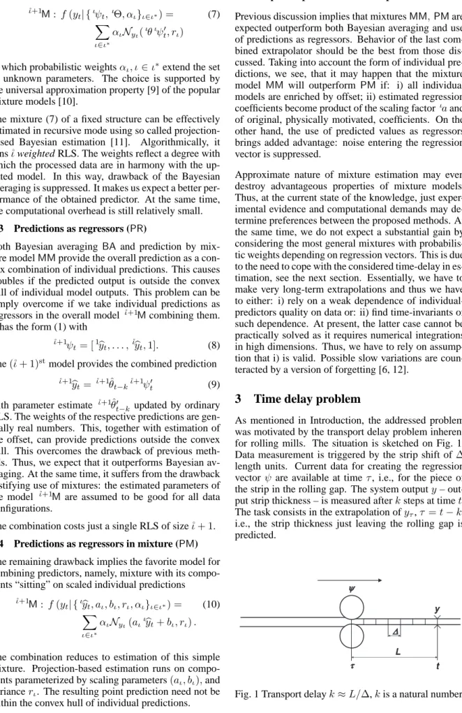
As mentioned in Introduction, the addressed problem was motivated by the transport delay problem inherent for rolling mills. The situation is sketched on Fig. 1. Data measurement is triggered by the strip shift of∆ length units. Current data for creating the regression vector ψare available at timeτ, i.e., for the piece of the strip in the rolling gap. The system outputy– out-put strip thickness – is measured afterksteps at timet. The task consists in the extrapolation ofyτ,τ =t−k, i.e., the strip thickness just leaving the rolling gap is predicted.
Estimates ιθˆ of ιθ parameterizing particular models ιM (1) can be updated at time t when the output y
t complements the regression vector ιψ
tinto data vector ιΨt = [y
t, ιψt]. For prediction at timeτ, justk-steps “old” parameter estimates and weights are available as indicated in (3). Utilization of the “old” parameters ob-viously deteriorates particular predictions. Therefore, the mixing of several predictions can be vital for coun-teracting this drawback.
4
Experiments
Experiments provide an insight into behavior of pro-posed methods and help us select the favorite one for the considered application. Moreover, they indicate whether the achieved improvement is worth increased computational demands. Comparisons are made on a typical data sample of the length 2000. In order to sup-press influence of the tuning phase, characteristics of predictions are computed for the last 1600 data records. Three underlying models ιMof the first order are used. They deal with the physical signals measured on the cold rolling mill. The signals are characterized in Ta-ble 1.
Tab. 1 Signals used in the combined models
No Meaning Units
1 output strip thickness µm 2 input strip thickness µm
3 rolling force MN
4 input strip speed m/s 5 output strip speed m/s 6 ratio of speeds
7 screwdown position µm
All models predict signal on channel 1. Structure of re-gression vectors of respective simple models, combin-ing the above channels and their delayed values, were determined from elementary physical laws, like mass conservation (mass-flow) principle, as well as from the inspection of extensive historical data. The transport delay between the rolling gap where prediction is made and the output measurements is k = 25. Thus pre-dictions are calculated with utilization ofk-step ”old” parameters and weights.
The processing imitated recursive real-time use. The respective simple models are estimated with forgetting factor 0.999. The compound models ˚ι+1M are
esti-mated with forgetting factor0.97.
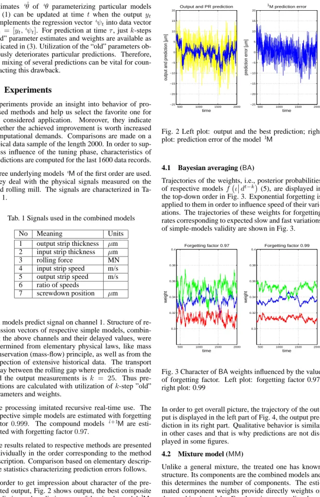
The results related to respective methods are presented individually in the order corresponding to the method description. Comparison based on elementary descrip-tive statistics characterizing prediction errors follows. In order to get impression about character of the pre-dicted output, Fig. 2 shows output, the best composite prediction and prediction error of the simple model 1M.
500 1000 1500 2000 −25 −20 −15 −10 −5 0 5 10 15 20
Output and PR prediction
time
output and prediction [
µ m] 500 1000 1500 2000 −25 −20 −15 −10 −5 0 5 10 15 20 1 M prediction error time prediction error [ µ m]
Fig. 2 Left plot: output and the best prediction; right plot: prediction error of the model 1M
4.1 Bayesian averaging (BA)
Trajectories of the weights, i.e., posterior probabilities of respective modelsf ιdt−k(5), are displayed in the top-down order in Fig. 3. Exponential forgetting is applied to them in order to influence speed of their vari-ations. The trajectories of these weights for forgetting rates corresponding to expected slow and fast variations of simple-models validity are shown in Fig. 3.
500 1000 1500 2000 0.3 0.32 0.34 0.36 0.38 0.4 Forgetting factor 0.97 time weight 500 1000 1500 2000 0.3 0.32 0.34 0.36 0.38 0.4 Forgetting factor 0.99 time weight
Fig. 3 Character ofBAweights influenced by the value
of forgetting factor. Left plot: forgetting factor 0.97, right plot: 0.99
In order to get overall picture, the trajectory of the out-put is displayed in the left part of Fig. 4, the outout-put pre-diction in its right part. Qualitative behavior is similar in other cases and that is why predictions are not dis-played in some figures.
4.2 Mixture model (MM)
Unlike a general mixture, the treated one has known structure. Its components are the combined models and this determines the number of components. The esti-mated component weights provide directly weights of the combined models. For the mixture, predicted and
500 1000 1500 2000 −25 −20 −15 −10 −5 0 5 10 15 20 Output time output [ µ m] 500 1000 1500 2000 −25 −20 −15 −10 −5 0 5 10 15 20 Prediction by BA time prediction [ µ m]
Fig. 4 System output (left plot) and itsBAprediction at the rolling gap (right plot)
observed properties may differ mainly due to the non-negligible error of approximate estimation. As seen in the overall comparison, Table 2, such a deterioration occurred but still the mixing provides observable im-provement comparing to individual models.
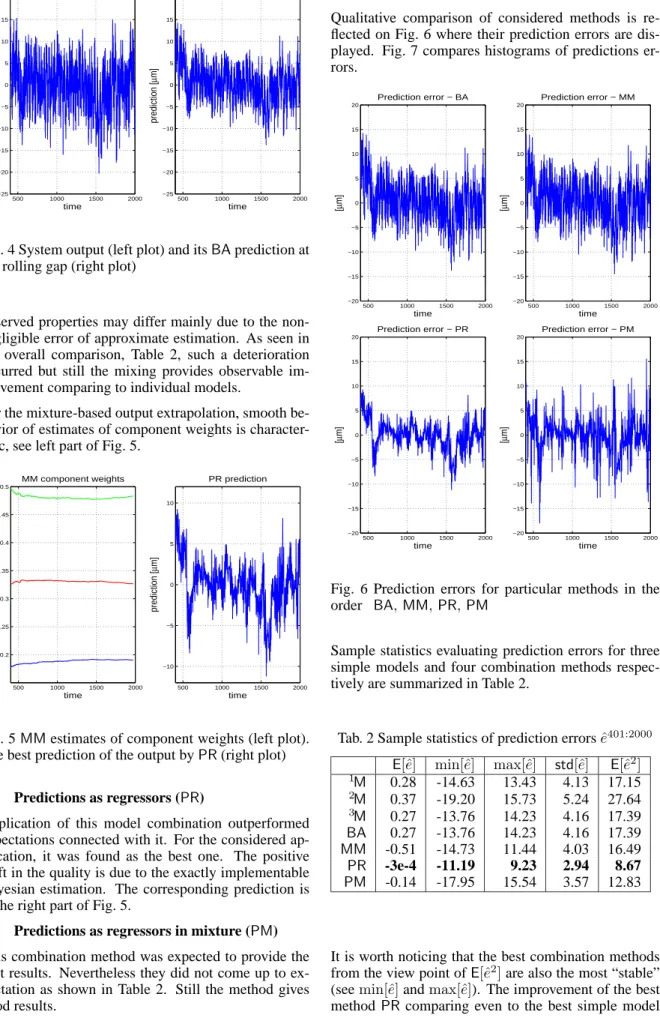
For the mixture-based output extrapolation, smooth be-havior of estimates of component weights is character-istic, see left part of Fig. 5.
500 1000 1500 2000 0.2 0.25 0.3 0.35 0.4 0.45 0.5 MM component weights time weight 500 1000 1500 2000 −10 −5 0 5 10 PR prediction time prediction [ µ m]
Fig. 5MMestimates of component weights (left plot). The best prediction of the output byPR(right plot)
4.3 Predictions as regressors (PR)
Application of this model combination outperformed expectations connected with it. For the considered ap-plication, it was found as the best one. The positive shift in the quality is due to the exactly implementable Bayesian estimation. The corresponding prediction is in the right part of Fig. 5.
4.4 Predictions as regressors in mixture (PM)
This combination method was expected to provide the best results. Nevertheless they did not come up to ex-pectation as shown in Table 2. Still the method gives good results.
4.5 Comparison of efficiency of respective methods
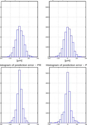
Qualitative comparison of considered methods is re-flected on Fig. 6 where their prediction errors are dis-played. Fig. 7 compares histograms of predictions er-rors. 500 1000 1500 2000 −20 −15 −10 −5 0 5 10 15 20 Prediction error − BA time [ µ m] 500 1000 1500 2000 −20 −15 −10 −5 0 5 10 15 20 Prediction error − MM time [ µ m] 500 1000 1500 2000 −20 −15 −10 −5 0 5 10 15 20 Prediction error − PR time [ µ m] 500 1000 1500 2000 −20 −15 −10 −5 0 5 10 15 20 Prediction error − PM time [ µ m]
Fig. 6 Prediction errors for particular methods in the order BA,MM,PR,PM
Sample statistics evaluating prediction errors for three simple models and four combination methods respec-tively are summarized in Table 2.
Tab. 2 Sample statistics of prediction errorseˆ401:2000
E[ˆe] min[ˆe] max[ˆe] std[ˆe] E[ˆe2] 1M 0.28 -14.63 13.43 4.13 17.15 2M 0.37 -19.20 15.73 5.24 27.64 3M 0.27 -13.76 14.23 4.16 17.39 BA 0.27 -13.76 14.23 4.16 17.39 MM -0.51 -14.73 11.44 4.03 16.49 PR -3e-4 -11.19 9.23 2.94 8.67 PM -0.14 -17.95 15.54 3.57 12.83
It is worth noticing that the best combination methods from the view point ofE[ˆe2]are also the most “stable”
(seemin[ˆe]andmax[ˆe]). The improvement of the best methodPR comparing even to the best simple model
−200 −10 0 10 20 100 200 300 400 500
Histogram of prediction error − BA
[µm] −200 −10 0 10 20 100 200 300 400 500
Histogram of prediction error − MM
[µm] −200 −10 0 10 20 100 200 300 400 500
Histogram of prediction error − PR
[µm] −200 −10 0 10 20 100 200 300 400 500
Histogram of prediction error − PM
[µm]
Fig. 7 Histograms of prediction errors for particular methods in the order BA,MM,PR,PM
1Mis obviously significant. Even the worst
combina-tion method achieves the quality comparable with the best simple model. This feature is important as the ob-served order of methods can be case dependent.
5
Conclusions
The paper presented four promising methods of com-bining outputs of physically motivated extrapolation models to a single one. For the considered rolling mill application, characterized by a significant transport de-lay, the combination of individual predictions by a static regression model seems to be the best solution. Due to the approximations involved, the result can be case de-pendent. Thus, the presented general discussion should be taken into account when tailoring the methods to other types of applications.
Acknowledgements
This work was partly supported by research projects BADDYR (grant 1ET100750401 of the Academy of Sciences of the Czech Republic) and DAR (project 1M0572 of the Czech Ministry of Education).
6
References
[1] V. Peterka, Bayesian system identification, Trends and Progress in System Identification, P. Eykhoff, Ed., pp. 239–304. Pergamon Press, Oxford, 1981. [2] L. Ljung, System Identification: Theory for the
User, Prentice-Hall, London, 1987.
[3] T. Bohlin, Interactive System Identification: Prospects and Pitfalls, Springer-Verlag, New York, 1991.
[4] G. Rath, Model Based Thickness Control of the Cold Strip Rolling Process, Doctoral Thesis, Uni-versity of Leoben, 2000.
[5] P. Ettler, M. K´arn´y and T. V. Guy, Bayes for rolling mills: From parameter estimation to deci-sion support, Proceedings of the 16th IFAC World Congress, Praha, 2005.
[6] M. K´arn´y, J. B¨ohm, T. V. Guy, L. Jirsa, I. Nagy, P. Nedoma, and L. Tesaˇr, Optimized Bayesian Dynamic Advising: Theory and Algorithms, Springer, London, 2005.
[7] M. K´arn´y, Algorithms for determining the model structure of a controlled system, Kybernetika, vol. 19, no. 2, pp. 164–178, 1983.
[8] A. E. Raftery, D. Madigan, and J. A. Hoeting, Bayesian model averaging for linear regression models, Journal of The American Statistical As-sociation, vol. 97, no. 437, pp. 179–191, 1997. [9] S. Haykin, Neural Networks: A Comprehensive
Foundation, Macmillan, New York, 1994. [10] D.M. Titterington, A.F.M. Smith, and U.E.
Makov, Statistical Analysis of Finite Mixtures, John Wiley, New York, 1985.
[11] J. Andr´ysek, Estimation of Dynamic Probabilis-tic Mixtures, PhD thesis, FJFI, ˇCVUT, POB 18, 18208 Prague 8, Czech Republic, 2005.
[12] R. Kulhav´y and M. B. Zarrop, On a general con-cept of forgetting, International Journal of Con-trol, vol. 58, no. 4, pp. 905–924, 1993.