Statistical Methods For Detecting Genetic Risk Factors of a Disease with Applications to Genome-Wide Association Studies

(1)

FACTORS OF A DISEASE WITH APPLICATIONS TO

GENOME-WIDE ASSOCIATION STUDIES

A THESIS SUBMITTED TO THE UNIVERSITY OF KENT FOR THE DEGREE OF DOCTOR OF PHILOSOPHY IN THE SUBJECT OF STATISTICS

BY FADHAA ALI

(2)

Acknowledgment

I would like to thank ministry of higher education and scientific research of Iraq (MOHESR) for funding this project. I would also like to thank Prof. Dankmar Böhning- University of Southampton and Dr. Fabrizio Leisen- University of Kent for accepting assessing my thesis and giving me a great feedback to improve it’s presentation.

I would like to thank many people in the School of Mathematics, Statistics and Actuarial sciences (SMSAS) at the University of Kent. Firstly, I would like to express my deepest gratefulness to my supervisor Prof. Jian Zhang for all the guidance that I received from him regarding my progress and for the positive feedback that I used to get from him. His advices took a significant part in enhancing my knowledge about this exciting research area and introduced me to all the drawbacks of my research that I might come across in the first place. I would also to thank my second advisor Dr. Xue Wang for reviewing my progress at some point and giving me great advices toward completion of my thesis.

During my Ph.D. study, I took valuable advantages from the magnificent Statis-tics Group in SMSAS and experienced the scientific atmosphere, which were reflected by the great seminar series on very wide range of statistical research areas. I would also like to express my warm thanks for all the Ph.D. students that I met within my time for their organising the wonderful students seminars that gave me a great opportunity to practice my presentation skills in several occasions.

Last but not the least, I would thank all the school administration officers for their unlimited support by providing me a great study environment. A special thank to the hard working lady whose name Claire Carter for her unlimited help since I started my Ph.D. in the School.

Lastly, I also feel very grateful to my family and all my dearest friends for all their supports and their caring about me in my very stressful time of my study.

(3)

Abstract

This thesis aims to develop various statistical methods for analysing the data derived from genome wide association studies (GWAS). The GWAS often involves genotyp-ing individual human genetic variation, usgenotyp-ing high-throughput genome-wide sgenotyp-ingle nucleotide polymorphism (SNP) arrays, in thousands of individuals and testing for association between those variants and a given disease under the assumption of common disease/common variant. Although GWAS have identified many potential genetic factors in the genome that affect the risks to complex diseases, there is still much of the genetic heritability that remains unexplained. The power of detecting new genetic risk variants can be improved by considering multiple genetic variants simultaneously with novel statistical methods. Improving the analysis of the GWAS data has received much attention from statisticians and other scientific researchers over the past decade.

There are several challenges arising in analysing the GWAS data. First, de-termining the risk SNPs might be difficult due to non-random correlation between SNPs that can inflate type I and II errors in statistical inference. When a group of SNPs are considered together in the context of haplotypes/genotypes, the distribu-tion of the haplotypes/genotypes is sparse, which makes it difficult to detect risk haplotypes/genotypes in terms of disease penetrance.

In this work, we proposed four new methods to identify risk haplotypes/genotypes based on their frequency differences between cases and controls. To evaluate the performances of our methods, we simulated datasets under wide range of scenarios according to both retrospective and prospective designs.

In the first method, we first reconstruct haplotypes by using unphased geno-types, followed by clustering and thresholding the inferred haplotypes into risk and non-risk groups with a two-component binomial-mixture model. In the method, the parameters were estimated by using the modified Expectation-Maximization al-gorithm, where the maximisation step was replaced the posterior sampling of the component parameters. We also elucidated the relationships between risk and non-risk haplotypes under different modes of inheritance and genotypic relative non-risk.

In the second method, we fitted a three-component mixture model to genotype data directly, followed by an odds-ratio thresholding.

In the third method, we combined the existing haplotype reconstruction software PHASE and permutation method to infer risk haplotypes.

(4)

In the fourth method, we proposed a new way to score the genotypes by clus-tering and combined it with a logistic regression approach to infer risk haplotypes.

The simulation studies showed that the first three methods outperformed the multiple testing method of (Zhu, 2010) in terms of average specificity and sen-sitivity (AVSS) in all scenarios considered. The logistic regression methods also outperformed the standard logistic regression method.

We applied our methods to two GWAS datasets on coronary artery disease (CAD) and hypertension (HT), detecting several new risk haplotypes and recovering a number of the existing disease-associated genetic variants in the literature.

(5)

1. Introduction . . . . 1

1.1 Genetic problems . . . 1

1.2 Statistical challenges . . . 1

1.3 Contributions of the thesis . . . 3

1.4 Arrangement of the thesis . . . 4

2. Background and Literature Review . . . . 5

2.1 Single-Nucleotide Polymorphism (SNP) . . . 5

2.1.1 Genotype/haplotype frequencies and their estimation . . . 7

2.1.2 Hardy-Weinberg Equilibrium . . . 8

2.2 Mode of inheritance . . . 9

2.3 Maximum likelihood method . . . 10

2.4 Finite mixture model . . . 11

2.4.1 Newton-Raphson algorithm . . . 12

2.4.2 EM algorithm . . . 13

2.5 Multi-locus haplotype inference . . . 14

2.5.1 Haplotype reconstructing . . . 14

2.5.2 SNP array segmentation . . . 17

(6)

2.6.1 Case-control studies of SNPs with a disease . . . 18

2.7 Haplotypes clustering . . . 20

2.7.1 Detecting disease-associated haplotypes . . . 20

2.7.2 Standard multiple logistic regression . . . 22

2.8 Study design . . . 25

2.8.1 Prospective studies . . . 26

2.8.2 Retrospective studies . . . 26

2.9 Specificity and sensitivity . . . 26

2.10 Population substructure . . . 27

2.11 Handling population substructure . . . 28

3. Haplotype mixture model-based approach (HM) . . . . 29

3.1 Introduction . . . 29

3.2 Methods . . . 31

3.2.1 Multiple testing method (MT) . . . 31

3.2.2 Mixture model-based method . . . 32

3.2.3 Example . . . 35

3.2.4 Improving the mixture approach . . . 36

3.2.5 Model justification . . . 38

3.2.6 Testing for haplotype inheritance modes . . . 40

3.3 Simulation studies . . . 41

3.3.1 Performance of the proposed Bayesian regularization . . . 42

3.3.2 Performance of the proposed hybrid mixture approach . . . . 43

(7)

3.4 Quality control of haplotypes . . . 51

3.5 Real data analysis . . . 52

3.6 Discussion and conclusion . . . 57

4. Genotype mixture model-based approach (GM) . . . . 59

4.2 Methodology . . . 61

4.2.1 Two-stage procedure . . . 61

4.2.2 Example . . . 64

4.2.3 EM algorithm initialization . . . 66

4.2.4 Multiple testing method . . . 67

4.3 Simulation studies . . . 67

4.3.1 Performance of the proposed data partition-based initialization 68 4.3.2 Performance of the proposed two-stage method . . . 69

5. Permutation approach . . . . 81

5.2 Method . . . 82

5.3 Simulation . . . 84

(8)

6.2 Method . . . 96

6.2.1 Clustering-based logistic method(CL) . . . 96

6.2.2 Standard multiple logistic method . . . 99

6.3 Simulation . . . 100

7. Discussions, conclusions and future works . . . . 108

7.1 Overview of the results of our methods . . . 108

(9)

2.1 The image from http://www.dnabaser.com/articles/SNP/SNP-single-nucleotide-polymorphism.html shows a segment of diploid DNA with

one SNP . . . 6

3.1 Performance of the three modification methods for Stage 1. The figures show the box-whisker plots of the estimated biases of the parameter θ, the averages of specificity and sensitivity, the attained log-likelihoods, and time-costs for the three modifications. . . 43 3.2 Performances of the proposed hybrid mixture method and the multiple

testing method on the cohort-design data with multiplicative or dominant or recessive inheritance models with sample size N = 5000.. . . 45 3.3 Performances of the proposed hybrid mixture method and the multiple

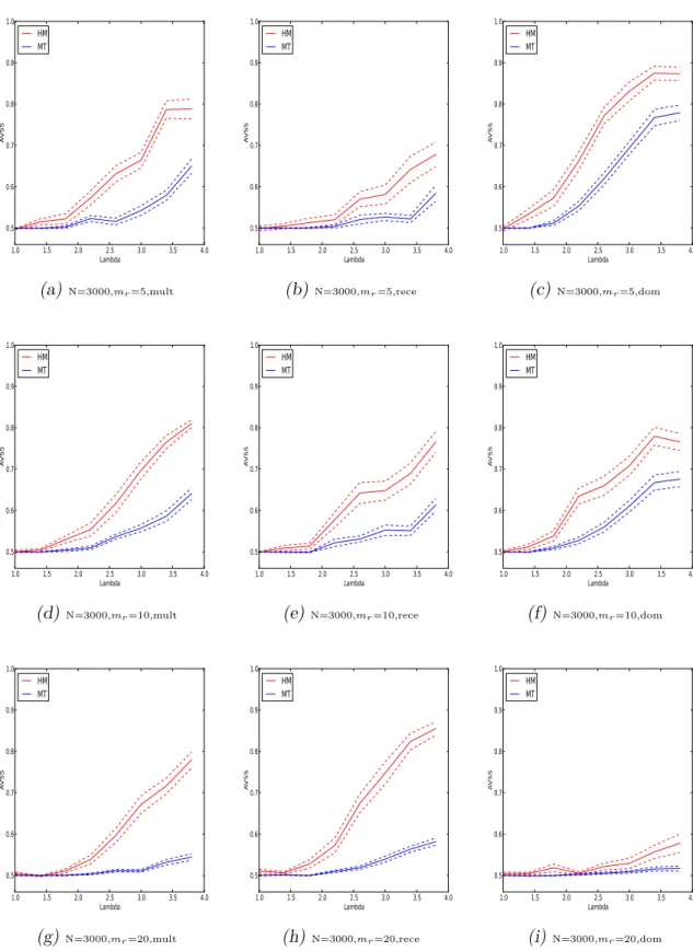
testing method on the cohort-design data with multiplicative or dominant or recessive inheritance models with sample size N = 3000.. . . 46 3.4 Performances of the proposed hybrid mixture and the multiple testing

method on the case-control data. . . 48 3.5 Performances of the proposed test for inheritance patterns. . . 50 3.6 The box-whisker plots of p-values of the chi-squared tests on 30 datasets

which represent the above six scenarios. . . 51

4.1 Performance of two initialization methods. . . 69 4.2 Performances of the proposed two-stage method and the multiple

test-ing method on the cohort-design data with multiplicative or dominant or recessive inheritance modes with sample size N = 5000. . . 71

(10)

4.3 Performances of the proposed two-stage method and the multiple test-ing method on the cohort-design data with multiplicative or dominant or recessive inheritance models with sample sizeN = 3000.. . . 72 4.4 Performances of the proposed two-stage method and the multiple testing

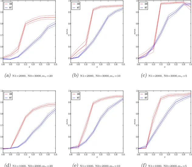
method on the case-control data. . . 74

5.1 Performances of the proposed permutation method and the multiple test-ing method on the cohort-design data with multiplicative or dominant or recessive inheritance models based on sample sizes of 5000. . . 86 5.2 Performances of the proposed permutation method and the multiple

test-ing method on the cohort-design data with multiplicative or dominant or recessive inheritance models based on sample sizes of 3000. . . 87 5.3 Performances of the proposed permutation method and the multiple

test-ing method on the case-control data. . . 89

6.1 Performances of CL method and SL method on the cohort-design data with multiplicative or dominant or recessive inheritance models with sample size

N = 5000. . . 101 6.2 Performances of CL method and SL method on the cohort-design data with

multiplicative or dominant or recessive inheritance models with sample size

N = 3000. . . 102 6.3 Performances of CL method and SL method on the case-control data. . . . 104

7.1 Performances of all methods on the cohort-design data with multiplicative or dominant or recessive inheritance modes based on sample sizes of 5000. The curves show the averages of the AVSS values over 30 replicates in each scenario for the methods HM, GM, MT, Per, CL, and SL. . . 110 7.2 Performances of all methods on the cohort-design data with multiplicative

or dominant or recessive inheritance modes based on sample sizes of 3000. The curves show the averages of the AVSS values over 30 replicates in each scenario for the methods HM, GM, MT, Per, CL, and SL. . . 111

(11)

7.3 Performances of all methods on the case-control data based on sample size 5000 or 3000. The curves show the averages of the AVSS values over 30 replicates in each scenario for the methods HM, GM, MT, Per, CL, and SL.112

(12)

2.1 Different sequences of two DNA segments of five individuals at the same positions on a chromosome pair. The segments comprise three SNPs at three loci coloured by different colours. Each SNP involves two alleles which are vary across individ-uals. The sequence of the three alleles at the same segment is called haplotype. Each pair of haplotypes is called genotype. . . 6 2.2 Contingency table of genotypes counts for Cases and Controls. In this table 1, 0

refer to genotypes counts in cases and controls respectively. . . 18

2.3 The contingency table of genotypic counts of a locus with two alleles C and T in a case-control sample. . . 19 2.4 Outcomes when clustering m hypotheses . . . 27

3.1 The table shows the first and the last iteration of the EM on

Exam-ple 3.2.3 starting from different random initial values. . . 36

3.2 The table shows the format of the genotype data format of WTCCC.

The first column represents the SNP id, the second column repre-sents individual id, the third column reprerepre-sents is the genotype of the corresponding at the corresponding individual and the score column shows the quality of SNPs calling. . . 52

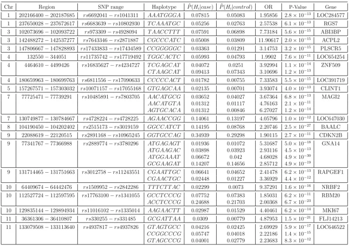
3.3 The predicted risk haplotypes for CAD by use of the WTCCC data.

In the table, the P-values were derived from the chi-square test of the

frequencies of Hi against the collapsed frequencies of the estimated

non-risk haplotypes. . . 54

(13)

3.5 The predicted risk haplotypes of hypertension by use of WTCCC data. In the table, the P-values were derived from the chi-square

test of the frequencies of Hi against the collapsed frequencies of the

estimated non-risk haplotypes. . . 56

3.6 The continuation of Table 3.5. . . 57

4.1 The table shows the random initial values and the estimated ones of

the final iteration when applying the EM algorithm to genotype data. 65

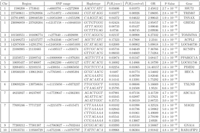
4.2 The predicted risk haplotypes for CAD by use of the WTCCC data.

In the table, the P-values were derived from the chi-squared test of the

frequencies of Hi against the collapsed frequencies of the estimated

non-risk haplotypes. . . 76

4.5 The predicted risk haplotypes of hypertension by use of WTCCC

data. In the table, the P-values were derived from the chi-squared

test of the frequencies of Hi against the collapsed frequencies of the

estimated non-risk haplotypes. . . 79

5.1 The suspicious regions for coronary artery disease of WTCCC data

detected by permutation method. . . 91

5.2 Continuation of Table 5.1. . . 92

5.3 The suspicious regions for hypertension of WTCCC data detected by

permutation method. . . 92

detected by the CL method. . . 106

6.3 The suspicious regions for hypertension of WTCCC data detected by

(14)

7.1 Potential risk genes for coronary artery disease and detection methods 114

(15)

1.1

Genetic problems

In the past decades, much attention has been paid to complex diseases such as coro-nary artery disease (CAD) and hypertension (HT), which are potentially caused by both genetic and environmental factors. The genetic factors are often attributed to genetic variants (or polymorphisms), the sites where genetic alleles are varying across individual genomes. It is well-known that although genetic variants can have undetectable marginal effects on the risk of a complex disease, they may have a significant effect as a group due to interactions between variants. Therefore, simul-taneously considering disease-associated variants can help us detect risk variants and develop medicines for curing the diseases. Multi-locus genotypes and haplotypes are commonly used to account for the interactions among the variants. Before the com-pletion of Human Genome Project, due to the limitation of biological technology, researchers were only able to focus their studies on a small proportion of regions in genome. After the completion of Human Genome Project, with developments insingle-nucleotide polymorphism (SNP)genotyping technology, genome-wide asso-ciation studies (GWAS) have become a feasible and powerful approach to uncover genetic variants with much better resolution by examining hundreds of thousands of SNPs distributed across the whole genome. Most of the existing genome-wide association studies are based on the hypothesis of common disease/common variant (CDCV). Despite the number of genetic variants identified, a large proportion of heritability has not been explained. Rare variants are believed to play an important role in the missing heritability. Studying rare variants and pinpointing the causal alleles accurately provide both opportunities and challenges to modern statistics.

1.2

Statistical challenges

One of early GWAS projects is theWelcome Trust Case Control Consortium(WTCCC)

(16)

more than 5×105 _{SNPs of more than 14000 unrelated cases (diseased}

individu-als) and 3000 unrelated shared controls (non-diseased individuindividu-als) were employed to find disease-associated variants for each disease. Significant progress has been made recently on analysing the WTCCC data (e.g., Kang et al., 2008; Zhu et al,

2010). Various statistical screenings based on odd ratio, logistic regressions,χ2 _and

Fisher’s exact tests have been conducted to identify the disease-associated SNPs of several complex diseases (Weir, 2005; Zhu et al., 2010; Burton et al., 2007).

Despite of this progress, analysing SNP data still faces a number of challenges related to the problems of missing data, low minor allele frequency, long distance correlation between SNPs, multiple test adjustments, and population substructures, data quality control, and among others. For example, in fitting a logistic regression model to genotypes, a large number of degrees of freedom will be involved, which may cause model over fitting. In contrast, fitting a logistic model to the corresponding hyplotypes is better because haplotypes have a lower dimensionality than genotypes. Unfortunately, as the haplotypes cannot be observed directly, they are required to infer from the unphased genotype data (Stephen, 2001). There are several software which can be used to reconstruct haplotypes from the unphased genotypes such as PHASE (Stephen, 2001) and the Expectation-Maximization (EM) (Excoffier and Slatkin, 1995). The disadvantage of using inferred haplotypes is uncertainty associ-ated with the above haplotype reconstructing process. In fact, the uncertainty may result in underestimating the variation in the data, inflating the type I error.

A closely related issue is the sparsity of genotype/haplotype distributions and high-dimensionality of genotypes/haplotypes, where the counts are often concen-trated on a few ones out of a large number of genotypes/haplotyeps. To address the issue, researchers have proposed variety of clustering-based methods. In these meth-ods, haplotypes/genotypes are divided into several subgroups or clusters based on their association with a disease. We assume that the haplotypes/genotypes within the same subgroup have the same risk probability of random effects (Templeton et al., 1987; Molitor et al., 2003; Zhu et al., 2010; Morris, 2005; 2006). Such methods are usually implemented via two or more stages: In the first stage, haplotypes or genotypes are grouped, while in the second stage the risk haplotypes are detected by using various test statistics, such as Z-tests and odd ratio tests. An alternative way is to fit a logistic regression model to clustered haplotypes rather than SNPs (Huang et al., 2011).

Modern statistics faces many challenges in analysing the GWAS data, which are summarised as follows.

(17)

1. Finding the causal SNPs of a disease can be difficult as these SNPs may be highly correlated with each other. This means even if we find that a SNP is associated with a disease, the risk may come from other SNPs nearby.

2. Considering multiple-SNP regions can give rise to the problem of high di-mensionality of genotypes/haplotypes. Yet, inference on risk variants may be difficult and inaccurate due to rarity of some haplotypes/genotypes.

3. Haplotype-structures are unknown in the real data as we observed SNP data in terms of genotypes only. Therefore, inferring their structures by using sta-tistical methodology such as PHASE may result in reconstructing uncertainty as pointed out before.

4. Non-diseased individuals (controls sample) in the real data come from different sub-populations, which will increase the false positive rate. Moreover, some of the SNP genotypes are of very low frequencies. As a result, significant differences between genotypes counts derived from different sub-populations. 5. Mode of inheritance can result in an increase of false discovery rate. For

example, a dominant mode can inflate type I error and recessive model can inflate type II error when the genotype relative risk (GRR) or the sample size is small.

1.3

Contributions of the thesis

This thesis aims to address the above challenges by considering a group of SNPs simultaneously. I will find the evidences about their associations with a disease of interest on the basis of both haplotypes and genotypes.

The contributions of this thesis are as follows: (1) I develop prospective mix-ture models for clustering haplotypes and genotypes and for identifying risk hap-lotypes. (2) I propose a new logistic regression model for genotypes. (3) I put forward a permutation-based approach for identifying risk haplotypes. A large sim-ulation studies have been conducted for the above methods and models under both prospective and retrospective settings. The proposed methods and models have been applied to the WTCCC data on CAD and hypertension, identifying a few more disease-associated haplotypes than in the literature.

(18)

1.4

Arrangement of the thesis

In Chapter 2, some genetic and statistical background are introduced and a lit-erature review on the topic is conducted. In Chapter 3, a novel two-component haplotype mixture model is proposed for clustering haplotypes and is applied to the simulated and real data sets on CAD and hypertension (HT). In Chapter 4, a novel three-component genotype mixture model is developed for detecting disease-associated haplotypes with applications to the simulated and real data sets. Two papers based on Chapters 3 and 4 have been submitted to two journals. In Chapter 5, a new permutation-based method is introduced and illustrated by applications to the simulated and real data sets. In Chapter 6, a new logistic regression model is proposed and evaluated by its applications to the simulated and real data sets. In Chapter 7, a conclusion is made for this thesis. In particular, a brief discussion on the quality of the results and on the advantages and disadvantages of the proposed methods are presented. The potential future work is also pointed out.

(19)

Population association studies are a key tool in determining genetic variants which affect the susceptibility to a complex disease. These variants can be produced by genetic drift, natural selection, mutation and recombination. The difference of an allele at a variant site in population groups reflects its associations with certain human trait. The higher the difference is, the more likely the genetic variant is associated with the trait.

Here, we focus on SNPs and their relationships to a disease and develop some statistical methods for this purpose. I start with an introduction to the background, followed by a literature review on the existing methods.

2.1

Single-Nucleotide Polymorphism (SNP)

Since a long time ago, geneticists have used phenotypes, protein sequencing, elec-trophoresis and microsatellites in order to detect the genetic differences across indi-viduals in terms of the deoxyribonucleic acid (DNA) sequences. After new biotech-nologies such as Microarrary Gene Chip being invented, detecting single-base dif-ferences has become possible in experiments under various biological conditions or different phenotypes (Kwok, 2003). Since then, the term of single-base differences in DNA amongst individuals has been known as single-nucleotide polymorphism (SNP) (and pronoun snip), see Figure (1.2). Each gene (or segment) in an entire DNA sequences often contains multiple SNPs.

As probable as it may seem, it has been proved beyond doubt that variations in genes may contribute to certain diseases. This can be seen from two aspects of genetic variants. Firstly, any disorder in DNA sequence can result in differences in gene regulations which in turn result in some diseases. Secondly, provided that some of chromosomes’ genes are coded for specific proteins, any variations in their SNP alleles may cause differences in their functions and their expressions (Balding et al., 2007).

(20)

Fig. 2.1: The image from http://www.dnabaser.com/articles/SNP/SNP-single-nucleotide-polymorphism.htmlshows a segment of diploid DNA with one SNP

Tab. 2.1: Different sequences of two DNA segments of five individuals at the same positions on a chromosome pair. The segments comprise three SNPs at three loci coloured by different colours. Each SNP involves two alleles which are vary across individuals. The sequence of the three alleles at the same segment is called haplotype. Each pair of haplotypes is called genotype.

Individuals chromosomes DNA segment with 3 loci haplotypes genotypes Individual 1 chromosome 1 ...ACCTGTAATCGGGTCA... TAT genotype 1

chromosome 2 ...ACCGGTATTCGGGCCA... GTC

Individual 2 chromosome 1 ...ACCTGTAATCGGGTCA... TAT genotype 2 chromosome 2 ...ACCTGTATTCGGGTCA... TTT

Individual 3 chromosome 1 ...ACCGGTATTCGGGCCA... GTC genotype 3 chromosome 2 ...ACCGGTATTCGGGCCA... GTC

Individual 4 chromosome 1 ...ACCTGTAATCGGGTCA... TAT genotype 4 chromosome 2 ...ACCTGTAATCGGGTCA... TAT

Individual 5 chromosome 1 ...ACCTGTAATCGGGTCA... TAT genotype 5 chromosome 2 ...ACCGGTATTCGGGTCA... GTT

The position of a SNP on a chromosome is so called locus (plural loci). Most of which are based on pair of alleles within a diploid chromosome. Each pair is so called genotype, whereas each allele is so called haplotype. The extension of the notion leads to multi-locus studies by which more than one locus is conducted for a study. A commonly way for detecting SNPs (or haplotypes) underlying a particular disease is to consider groups of individuals under different conditions or traits (Weir, 1996).

(21)

2.1.1 Genotype/haplotype frequencies and their estimation

Suppose that we have a sample of genotype observations on a binary locus with

alleles C and T for N individuals in a sample with counts n1, n2 and population

frequenciesp1, p2, respectively. The possible genotypes for this locus will be CC, CT

and TT. Let the genotype counts denoted byN1, N2, N3 with population frequencies

q1, q2, q3. The counts of these genotypes are random variables following multinomial

distribution (Weir, 1996). Pr(N1, N2, N3) = N! N1!N2!N3! qN1 1 q N2 2 q N3 3 ,

whereas the distribution of alleles C and T is binomial, which can be written as

Pr(n1, n2) =

(2N)!

n1!n2!

pn1

1 pn22.

We can then derive the relationship of genotypes and haplotypes counts(or frequen-cies) as follows: n1 = 2N1+N2 and n2 = 2N3+N2, (2.1) N =N1+N2+N3, n1 +n2 = 2N. Similarly, p1 =q1+ 1 2q2, p2 =q3+ 1 2q2, (2.2) where q1+q2+q3 =p1+p2 = 1.

However, in many cases, the population frequencies of genotypes as well as their alleles are unknown, so we may use their sample counts to estimate them by

ˆ p1 = n1 2N and ˆq1 = N1 N . (2.3)

The above model and estimation can be easily extended to the case of multiple-locus genotypes/haplotypes, where a multinomial model is required.

Many other methods have been introduced to estimate population frequencies such as Maximum Likelihood Estimation (Weir, 1996; Excoffier and Slatkin, 1995; McLachlan and Peel, 2003). We will use some of them in the upcoming chapters.

(22)

2.1.2 Hardy-Weinberg Equilibrium

The relationship between the frequencies of the genotypes and their haplotypes is important as far as association with diseases is concerned. Therefore, Hardy (1877-1947) and Weinberg (1862-1937) independently formulated what is now called Hardy-Weinberg model in 1908. The mathematical relationship between the fre-quencies of the single-locus genotypes and haplotypes can be described by:

q1 =p21;q2 = 2p1p2;q3 =p22,

for a given SNP on a chromosome with two allelesCandT.Hardy-Weinberg

Equilib-rium (HWE) can be applicable only when some assumptions hold in the population (Hartl and Clark, 1997). These assumptions include that (1) the individuals under study should be diploid; (2) no overlapping exists amongst generations; (3) muta-tion is not important; (4) alleles under study are not affected by natural selecmuta-tion; (5) migration is trivial; (6) the size of population is large; (7) individuals are mated randomly; and (8) SNPs are biallelic (involve two alleles only). If any of these assumptions is not true, we then say the population under Hardy-Weinberg disequi-librium, by which the alleles of a particular locus or the haplotypes of multi-locus regions are not under random mating (Weir, 1996 ). The mathematical relationship between genotypes and alleles frequencies is given by

q1 =p21+DC;q2 = 2p1p2−2DC;q3 =p22+DC,

which implies

DC =q1−p21,

whereDC is called disequilibrium coefficient. The MLE of DC is

ˆ

DC = ˆq1−pˆ21.

The expected value of this estimation can be calculated by the formulas

E( ˆDC) =DC+ 1 2N[p1(1−p1) +DC], and V ar( ˆDC) = 1 N[p 2 1(1−p1)2 + (1−2p1)2DC −DC2].

The latter formula can be simplified by using Fisher variance approximation ˆ

(23)

provided the sample size is relatively large. Hence, under the null hypothesis H0 :

DC = 0, the following statistics

z =

ˆ

DC −E( ˆDC)

q

V ar( ˆDC)

is distributed as standard normal. We can use this as a test statistic to find out whether a population is under HWE or not. This is equivalent to testing the null

hypothesis H0 : DC = 0. Additionally, there are two more tests which can be

used for the same purpose, namely, Fisher exact test and likelihood ratio test. The HWE can be extended to the case of multiple-locus genotypes/haplotypes in terms of random mating.

HWE is an important assumption in testing the association between the frequen-cies of the haplotypes and the phenotypes under the null hypothesis of no association between them. If the association is found, the proportion of genotypes (or haplo-types) in cases will then differ significantly from the ones in controls. Furihata, Ito and Kamatani (2006) found a method, which is so called likelihood-based algo-rithm PENHAPLO, to test the association when the HWE assumption was invalid in cases.

2.2

Mode of inheritance

Mode of inheritance refers to the way that genetic variants affect the probability of being diseased. It can be determined by a function that is so called penetrance by which the conditional probability of being affected, given a specific genotype. There are several modes which can be defined according to the relationships between haplotype risks and genotype risks. For simplicity, we consider a single-locus with two alleles (or haplotyopes). Let allele D be the risk allele and N be the non-risk allele. The possible genotypes will be DD, ND and NN. We can then define the penetrance functions as follows:

f0 =P( affected |N N), f1 =P( affected|N D) and f2 =P( affected |DD)

Letλ denote the genotypic relative risk (GRR), so that

λ= P( affected|DD)

(24)

Hence, modes of inheritance can be defined as follows (Hartl and Clark, 1997):

1. Dominant model: The risk of getting disease will increase in amount of λ,

given the individual’s genotype is type ND or DD.

f2 =f1 =λf0.

2. Recessive model: The risk of getting disease will increase in amount ofλ, given

the individual’s genotype is only type DD.

f2 =λf0, f1 =f0.

3. Multiplicative model: The risk of getting disease will increase in amount ofλ,

given the individual’s genotype is type DD and in amount of √λ, given the

individual’s genotype is type ND.

f2 =λf0, f1 =

√

λf0

The notation can be easily extended to the case of multiple-locus genotypes/haplotypes (Hartl and Danial, 1997).

2.3

Maximum likelihood method

The maximum likelihood method is the most common method for estimating param-eters in a parametric model. Let us consider the locus we mentioned in Section 2.1.1. The likelihood function can be written as

L(pc) = (2N)! n1!n2! p1n1(1−p1)(n2), where 2N =n1+n2 and p1 +p2 = 1.

The log-likelihood function can be written as

logL(p1) =c+n1logp1+n2log(1−p1),

(25)

On equating

∂logL(p1)

∂p1

to zero and solving the equation, we have

∂(p1) ∂p1 = n1 p1 − n2 1−p1 = 0 ⇒pˆ1 = n1 2N. Similarly, we have ˆ p2 = n2 2N.

2.4

Finite mixture model

Let n1, n2, ..., nJ denote a random sample of size N, where nj,1 ≤ j ≤ J is a

d-dimensional random vector with probability density functionf(nj;θ) on<d.

Sup-pose that nj can be classified into k subgroups based on the similarity and the

dissimilarity of these observations. This can easily be conducted by using the mix-ture model given by

f(nj;θ) =

k

X

i=1

πif(nj;pi),

whereθ = (π1, ..., πk−1;p1, ..., pk)T,andkis the number of components in the model,

0≤πi ≤1 is the mixed weights and Pki=1πi = 1.

The likelihood of θ given data n can be calculated by

L(θ|n) = J Y j=1 k X i=1 πif(nj;pi), (2.4)

The log likelihood can be written as

l(θ|n) = J X j=1 log k X i=1 πif(nj;pi), (2.5)

(26)

formulate the complete one, we need to define group membership indicators. For simplicity, let us assume that k=2 when we are interested in finding the risk and

non-risk haplotypes. The haplotypes can be denoted by {Hj,1 ≤ j ≤ J}, and

θ = (π, pr, pTr), where pr, pr refer to risk and non-risk haplotype group, respectively.

With that, group membership indicators can be defined byIjr and Ijr¯,

Ijr =

  

1, Hj in the risk group

0, otherwise , Ijr¯=

  

1, Hj in the non-risk group

0, otherwise

for 1≤j ≤J. Set I={(Ijr, Ijr¯)T : 1≤j ≤J}.

To this end, the log-likelihood in the equation 2.5 can be written as

l(θ|n,I) = J X j=1 n Ijrlog(πf((n0j, n1j)T|pr)) +Ijr¯log((1−π)f((n0j, n1j)T|pr¯)) o , (2.6) wherenj =n0j+n1j.

Calculating the maximum likelihood estimation ofθcan be difficult analytically.

Therefore, some of iterative methods can be employed to calculate the ML estima-tors numerically. A common way is by employing Newton raphson method or EM algorithm.

2.4.1 Newton-Raphson algorithm

Given the incomplete likelihood in the equation 2.5, Newton-raphson method can be

used to find the ML ofθ. To illustrate the basic idea behind it, letS(n;θ) denote the

score and M(θ;n) denote (Fisher) information matrix of the log-likelihood in 2.5,

whereθ = (π, pr, pr¯). We then have S(n;θ) = (∂l ∂π, ∂l ∂pr , ∂l ∂pr¯ )T, and M(θ;n) =      −∂2_l ∂π2 − ∂2_l ∂π∂pr − ∂2_l ∂πpr¯ − ∂2_l ∂π∂pr − ∂2_l ∂p2 r − ∂2_l ∂pr∂pr¯ − ∂2_l ∂π∂pr¯ − ∂2_l ∂pr∂p¯r − ∂2_l ∂p2 ¯ r      .

By Taylor’s theorem, we can expand the derivative of the log-likelihood aroundθ(t).

This gives

(27)

Solving the above equation gives

θ(t+1) =θt+M−1(θ(t);n)S(n;θ(t)).

We repeat these steps until getting convergence to certain values (McLachlan and Krishnan, 2008).

2.4.2 EM algorithm

EM algorithm is an iterative method to find ML ofθby maximising the log-likelihood

in (2.6). This algorithm can be performed in two steps: expectation step and

maximization step (McLachlan and Peel, 2000a). Given the current valueθ(t) _{= (}_p(t)

r , p (t) ¯

r , π(t))T and the datan, we first calculate

the current log-likelihoodl(θ(t)_|_n_{). Then, in the E-step, we calculate the expectation}

of the complete-data log-likelihood with respect to I,

In the M-step, we update θ(t) _{by solving the partial derivatives equations}

∂Q ∂π = 0, ∂Q ∂pr = 0, ∂Q ∂p¯r = 0. We obtain π(t+1) = PJ j=1τ (t) jr J , p (t+1) r = PJ j=1τ (t) jrn1j PJ j=1τ (t) jr(n1j +n0j) , p(_¯_rt+1) = PJ j=1τ (t) jr¯n1j PJ j=1τ (t) j¯r(n1j+n0j) .

(28)

non-risk groups. Based on τ_jr(t+1) and τ_j(_¯_rt+1), the estimated risk and non-risk haplotype clusters can be defined by

S_r(t+1) ={Hj :τ (t+1) jr > τ (t+1) j¯r }, S (t+1) ¯ r ={Hj :τ (t+1) jr ≤τ (t+1) j¯r }.

We will show how this algorithm works practically in our approach as we use it to estimate parameters of interest.

2.5

Multi-locus haplotype inference

A sequence of the alleles at different loci on a chromosome is so called haplotype. As each locus is based on two alleles, the possible number of different haplotypes

resulted fromkSNPs will be 2k_{. Haplotypes-based studies are more important than}

studying SNPs as the latter do not account for the joint behavior of SNPs very well when they are highly correlated to each other. However, we might find evidence of association for one haplotype or many by conducting simultaneous analyses of multiple SNPs that may jointly provide such evidence.

The functional aspects of protein are identified by a sequence of amino acids, corresponding to DNA variations on a haplotype (Clark, 2004). However, in most (if not all ) of these studies, haplotypes are generally unknown. Therefore we need to infer them by using available or known genotype data by using some programs such as PHASE (Stephens et al., 2001) or fastPHASE (Scheet and Stephens, 2006) which implement a bayesian framework to phase estimation.

2.5.1 Haplotype reconstructing

Excoffier and Slatkin(1995) proposed a method to reconstruct haplotypes.

As-sume that a sample of n diploid individuals are observations from a population.

Let G = (G1, G2, ..., Gn) denote the genotypes for these individuals, and H =

(H1, H2, ...., Hn) the unknown haplotype pairs that producedG, whereHj = (H1j, H2j).

Let h = (h1, h2, ...., hk) denote all possible haplotypes that can result in G and

p= (p1, p2, ..., pk) be the unknown population frequencies ofh. Thus, we can write

the maximum likelihood function as follows

L(p|G) =P(G|p) =

n

Y

i=1

(29)

Under HWE, P(Gi|p) = mi X j=1 P(H_ij₁)P(H_ij₂),

where mi = 2ti−1, and ti is the number of heterozygots in the genotype Gi. To

clarify this point, suppose we have a setG consists of 4 individuals genotypes such

as

G={(2,1,0,2)T,(1,1,0,0)T,(1,0,0,1)T,(0,2,2,1)T},

where 0,1 refers to homozygots and 2 refers to heterozygots (Zhang et al., 2005).

In this genotype, there are two heterozygots in this genotype which means it can be decomposed into 4 possible ways. In addition, there are 8 different haplotypes

that can result in G. Therefore, the possible different haplotypes will be h={h1 =

(0,1,0,0), h2 = (1,1,0,1), h3 = (0,1,0,1), h4 = (1,1,0,0), h5 = (1,0,0,1), h6 =

(0,0,0,1), h7 = (0,1,1,1), h8 = (0,0,1,1)}, and the 4 possible ways, namely

assign-ments, that we can decomposeG into are as follows

H1 ={(h1, h2),(h4, h4),(h5, h5),(h6, h7)}

H2 ={(h1, h2),(h4, h4),(h5, h5),(h3, h8)}

H3 ={(h3, h4),(h4, h4),(h5, h5),(h6, h7)}

H4 ={(h3, h4),(h4, h4),(h5, h5),(h3, h8)}

We use the EM algorithm to estimate the parameters pi’s. We define an indicator

vectorZ = (Z1, Z2, ..., Zn), where Zi = (Zi1, Zi2, ...., Zimi),

zij =

  

1, if haplotype pair (H_ij₁, H_ij₂) consistent with Gi

0, otherwise (2.7)

Hence, the complete likelihood can be written as

L(p,Z,G) = n Y i=1 mi Y j=1 [P(H_ij₁)P(H_ij₂)]Zij_,

and the log-likelihood can be written as

logL(p,Z,G) = n X i=1 mi X j=1 Zijlog[P(Hij1)P(H j i2)].

(30)

E-Step: Q(θ, θ(t)) =E[logL(p,Z|G)|p(t)] = n X i=1 mi X j=1 ˆ Zij[P(Hij1)P(H j i2)].

We can calculate ˆZij by using the conditional expectation,

Similarly, we can calculate [ ˆP(H_ij)](t) _{as follows}

[ ˆP(H_ij)](t) =E(H_ij|Zij = 1,G, p, p(t)) = P(Gi|H j i, Zij = 1, p, p(t))P(H j i|Zij = 1, p(t)) P(Gi|p) = P(Gi|H j i, Zij = 1, p, p(t))(P(Hij1)) (t) (P(H_ij₂))(t) Pmi j=1(P(H j i1)) (t)(P(H_ij₂))(t) , whereH_ij = (H_ij₁, H_ij₂).

M-Step: We use gene count method to calculate the population frequencies as follows ˆ p(_`t+1) = 1 2 n X i=1 mi X j=1 xij[ ˆP(Hij)] (t)_,

wherexij = 0,1,2 depends on how many times the haplotypeh`present in haplotype

pair H_ij, `= 1,2, ...., k.

To this end, we can use the calculated frequencies to choose ˆH to maximize

P(H|ˆp,G). That is, by choosing the most probable haplotype assignment, given

the genotype data. However, within this procedure, it is not clear how best to re-construct haplotypes. Stephen, Smith and Donnelly (2001) develop a new technique to reconstruct haplotypes by using Gibbs Sampling, a type of MCMC algorithm.

(31)

sta-tionary distributionP(H|G), in light of all possible haplotype reconstructions. The steps of their algorithm are as follows:

We assign an initial haplotypes reconstructionH(0)_{. We then choose an}

individ-ual ,i, uniformly and at random from all ambiguous individindivid-uals. We next sample

H_i(t+1) fromP(Hi|G, H−(ti)), whereH−i is the set of haplotypes excluding individual i.

Having done that, we setH_j(t+1) =H_j(t) for j = 1,2.., n, j 6=i. We repeat these steps

enough times until we get a convergence. However, the distribution P(Hi|G, H−i)

is not even known for most models, so that Stephens, Smith and Donnelly (2001) found out it would be helpful to use the constructing full-conditional distribution for any haplotype pairHi = (hi1, hi2) that consistent withGi. That is,

P(Hi|G, H−i)∝P(Hi|H−i)∝ψ(hi1|H−i)ψ(hi2|H−i, hi1),

whereψ(.|H) is the conditional distribution of a future sampled haplotype, given a

setHof previously sampled haplotypes. This distribution is also not known

gener-ally in many occasions. However, it is known in special case of parent-independent mutation which means that the type of a mutant offspring and the type of parent are

independent. To improve and fasten the procedure, we calculate ψ(h|H) as follows

ψ(h|H) = X α∈E ∞ X s=0 rα r ( θ r+θ) s r r+θ(P s₎ αh,

where r is the total number of haplotypes in H, rα is the number of haplotypes

of type α in the set H, E refers to the countable set of types of mutation models,

θ is the scaled mutation rate, s is sampled from geometric distribution, and P is

the(reversible) mutation matrix.

2.5.2 SNP array segmentation

A large number of SNPs can result in sparsely distributed haplotypes with many rare haplotypes, which makes it difficult to detect their associations with the disease. Therefore, some statistical approaches are required to handle the rare haplotypes for complex traits in a population. The existing methods include the two-stage (or multiple Z-testing) method (Zhu et al., 2010), sibpair and odds ratio weighted sum statistics (SPWSS,ORWSS) (Feng et al., 2011), and weighted haplotype and imputation-based test (Li et al., 2010). Detecting the associations of haplotypes with the disease by using conventional statistics such as chi-square test and odds ratio test can suffer from the problem of multiple testing adjustment due to the high

(32)

dimensionality of haplotypes. To overcome the above limitation, in this thesis, I first segmentate the SNP array and then reduce the number of tests by use of clustered haplotypes/genotypes, rather than individual haplotypes/genotypes.

2.6

Genome-wide association studies

Genome-wide association studies (GWAS) have played an important role in identify-ing genetic polymorphisms contributidentify-ing to complex human diseases. With the rapid pace of developing SNP genotyping technology, a large number of markers (some times greater than 500000) have been considered by many researchers for a large number of individuals to investigate the effects of genetic variants on diseases. The earlier studies have focused on multiple single-locus analyses with an appropriate adjustment for multiple testing effects (Balding et al., 2007).

The problems of high dimensionality, sparsity problems, and linkage disequilib-rium can arise from GWAS. In the following sub-section, I will review some existing methods of detecting rare risk variants.

2.6.1 Case-control studies of SNPs with a disease

Studying contributions of SNPs to a disease can be performed by taking two samples of individuals from a population: one with the disease(cases) and the other without the disease (control). For simplicity, assume that the alleles of the suspicious SNP

are {C, T}. But the following tests can be extended to the case of multiple-loci.

We use chi-square to test the null hypothesis of no association between SNP and disease. To do so, we represent a contingency table of the observed and the expected genotypes counts for cases and controls (see table (2.2)).

Tab. 2.2: Contingency table of genotypes counts for Cases and Controls. In this table 1, 0 refer to genotypes counts in cases and controls respectively.

Case Control Genotype CC CT T T CC CT T T Observed counts n1 CC n1CT n1T T n0CC n0CT n0T T Expected counts n1_[˜_p2 C]1 2n1[˜pC(1−p˜C)]1 n1[(1−p˜C)2]1 n0[˜p2C]0 2n0[˜pC(1−p˜C)]0 n0[(1−p˜C)2]0 Observed-Expected n1_D_ˆ1 C −2n 1_D_ˆ1 C n 1_D_ˆ1 C n 0_D_ˆ0 C −2n 0_D_ˆ0 C n 0_D_ˆ0 C

(33)

. The chi-square test can be calculated by χ2 = X cases X genotypes (Observed−Expected)2 Expected .

We compare the value of the observed test with the tabled one derived from Chi-square distribution of 2 degrees of freedom. However, if there is any of the classes in the table with count less than 5, we will then get non-significant value for the test statistic despite the fact that the SNP could be associated with disease. For this

reason, we need to use a continuity correction of 0.5 in the numerator of chi-square

to overcome such problem (Yates, 1934).

χ2 = X cases X genotypes (|Observed−Expected| −0.5)2 Expected

In many cases, some diseases can result from more than one SNP. Therefore, some statistical methods are needed to detect the association between SNPs and disease such as multi loci(or haplotype) methods. We will mention some of these methods in the coming sections.

In addition, we can use Fisher’s exact test to detect the association, most com-monly, when we have one of the classes has count less than five. We can fit the contingency table of the genotypic counts in the cases and the controls as shown in Table 2.3.

Tab. 2.3: The contingency table of genotypic counts of a locus with two alleles C and T in a case-control sample. Genotype CC CT TT Total Case n1_CC n1_CT n1_{T T} ncase Control n0 CC n0CT n0T T ncontrol Total nCC nCT nT T N

We calculate thep as follows

p= ncase!ncontrol! nCC!nCT! nT T!

N!n0

CC! n0CT!n0T T!n1CC!n1CT!n1T T!

. (2.8)

We then need to form all the other samples that follow the prospective and

retro-spective distribution of the observed data in Table 2.3. We calculate{pi}of all these

samples by using 2.8. The fisher’s exact test equal to P

pi≤ppi.

(34)

2.7

Haplotypes clustering

A challenging issue with haplotype-based analyses is the lack of enough phase in-formation to reconstruct haplotypes as many haplotypes may be consistent with unphased genotype data. Rarity is another drawback that we need to cope with when conducting haplotype-based inference. Several methods in the literature have been proposed based on classifying haplotypes according to some similarities into several subgroups and assume the haplotypes of each subgroup have the same effect on disease prevalence in the sample (Templeton et al., 1987; Molitor et al., 2003; Morris, 2005; 2006). Zhu et al. (2010) have proposed a multiple testing method to co-classify the haplotypes in selected subsample based on the difference between

P(haplotype|cases) and P(haplotype|controls) in the first stage of his method.

Fitting a logistic regression model to the clustered haplotypes can be more effi-cient rather than SNPs in measuring their association with a disease (Huang et al., 2011), as the haplotypes can be more informative than SNPs in terms of underlying biological relationships with the disease. However, the rarity and high dimensional-ity are also challenges in the logistic regression-based analyses (Igo et al., 2009) as they can result in a high degree of freedom that can undermine the estimation of the parameters. In the following two subsections, we will describe briefly the method of Zhu et al. (2010) and the method of the standard logistic regression.

2.7.1 Detecting disease-associated haplotypes Multiple testing method

Zhu et al. (2010) proposed a method to detect the association between disease and unrelated cases as well as affected sibpairs. This method can be done through two stages. The former stage represents co-classifying the rare risk haplotypes in unrelated cases as well as affected sibpairs. The latter stage represents using Fisher’s exact test to find out whether the co-classifying haplotypes are associated with particular disease or not.

Assume that we examine the association of haplotypes with a disease. We first

letH={H1, H2, ..., Hn}be a set of risk haplotypes with corresponding haplotypes

frequenciesp1, p2, ..., pn in affected cases andp10, p02, ..., p0n in controls, and letHn+1

be the rest of the non-risk haplotypes with the total frequency pn+1 in cases and

p0

(35)

p=Pn

i=1pi. Let f2, f1, f0 be the three penetrances and defined as follows f2 =Pr(affected|HiHj),

f1 =Pr(affected|HiHn+1),

and

f0 =Pr(affected|Hn+1Hn+1),

wherei, j = 1,2, ...., n.

We can then calculate the frequency of a rare risk haplotype Hi in cases as

follows: hi =Pr(Hi|affected) = Pr(HiHi|affected) + 0.5 X j6=i Pr(HiHj|affected) = f2Pr(HiHi) + 0.5 P j6=i,j≤nf2Pr(HiHj) + 0.5f1Pr(HiHn+1) Pr(affected) = f2Pr(HiHi) + 0.5 P j6=i,j≤nf2)Pr(HiHj) + 0.5f1Pr(HiHn+1) Pn i=1 Pn j=1f2Pr(HiHi) +Pni=1f1Pr(HiHn+1) +f0Pr(Hn+1Hn+1)

Given the penetrances, we have

hi =Pr(Hi|affected) = f2p0ip0i +f2p0i(p−p0i) +f1p0i(1−p) f2p2+f12p(1−p) +f0(1−p)2 = f2p 0 ip+f1p0i(1−p) f2p2₊_f1₂_p₍₁₋_p_{) +}_f0₍₁₋_p₎2.

Since we study rare risk haplotypes within a family. It is helpful to consider mode of inheritance. In the multiplicative mode, we assume that

f2 =ηf0, f1 = √ ηf0, which imply Pr(Hi|af f ected) = ηf0p0ip+ √ ηf0p0i(1−p) ηf0p2+ 2 √ ηf0p(1−p) +f0(1−p)2 = ηp 0 ip+ √ ηp0_i(1−p) ηp2_{+ 2}√_ηp₍₁₋_p_{) + (1}₋_p₎2 = [ √ ηp+ (1−p)]√ηp0 i [√ηp+ (1−p)]2 = √ ηp0 i √ ηp+ (1−p).

(36)

In the Dominant mode, we suppose that f2 =f1 =ηf0, which imply Pr(Hi|af f ected) = ηf0p0ip+ηf0p0i(1−p) ηf0p2+ 2ηf0p(1−p) +f0(1−p)2 = ηp 0 i ηp(2−p) + (1−p)2.

In the recessive mode, we suppose that

f2 =ηf0, f1 =f0, which implies Pr(Hi|af f ected) = ηf0p0ip+f0p0i(1−p) ηf0p2 _{+ 2}_f0p₍₁₋_p_{) +}_f0₍₁₋_p₎2 = [p(η−1) + 1]p0 i p2₍_η₋_{1) + 1} .

At stage 1 of this method, the risk setS can be defined as

S ={Hi|hi−h0i > µ

s

h0

i(1−h0i)

2N },

where N is the number of cases used for co-classification,µis a predefined constant

andhiis the frequency of rare risk haplotypeHiin unrelated cases. We can estimate

h0_i from controls, if it is unknown practically. At stage 2, we use the remaining cases

and controls to refine the haplotypes inS by using fisher’s exact test.

2.7.2 Standard multiple logistic regression

Many studies in the literature have used the standard multiple logistic regression (SL) to analyse the genotype data. In this subsection, we review a standard way of fitting the logistic regression to the data in order to find the disease-associated genotypes (David et al., 2000). The multiple logistic regression model can be written as follows. log p(Xi) 1−p(Xi) =β0+ J X j=1 βjxij, (2.9)

(37)

where 1≤i ≤n, and Xi = (xi1, xi2, ..., xiJ)T, namely the design variables, J is the

total number of genotypes under study andn is the total number of the individuals.

Here, p(Xi) can be calculated by

p(Xi) = eβ0+PJ_j₌₁βjxij 1 +eβ0+P J j=1βjxij . (2.10)

Generally, in the logistic regression model, if there are J design variables with J

values, thenJ−1 design variables will be needed to allow an automatic adjustment

for the intercept coefficient β0. Therefore, we let xij,1 ≤ j ≤ J −1 take 1 if the

genotypeGj is present in the individual i and 0 if not. Let β= (β0, β1, ..., βJ)T

The likelihood equations may be expressed as follows

L(β) =

n

Y

i=1

p(Xi)yi(1−p(Xi))(1−yi)

and the log-likelihood can be calculated by

l(β) =

n

X

i=1

{yilogp(Xi) + (1−yi) log(1−p(Xi))}.

On equating the first derivative ofl(β) to zero, we find

n X i=1 (yi−p(Xi)) = 0 and n X i=1 xij(yi−p(Xi)) = 0

forj = 0,1,2, ..., J.Let ˆβ = ( ˆβ0,β1, ...,ˆ βˆJ)T denote the solution for these equations.

As each individual will have only one genotypes, the covariances of ˆβ will be

zeros, whereas the variances can be expressed as follows:

∂2L(β) ∂β2 j =− n X i=1 x2_ijp(Xi)(1−p(Xi))

The observed information matrix M(β) will only have the variances of ˆβ, and the

estimated standard error of the estimated coefficients will be expressed as follows:

d SE( ˆβj) = h d V ar( ˆβj) i1/2 ,

(38)

for j = 0,1, ..., J. To this end, finding the importance of the exposure variables in the model needs to perform a test statistics. The most used ones are likelihood ratio test, Wald statistics. The likelihood ratio test can be written as

ωj =−2 log(

L0

Lj

),

whereL0 denote the likelihood of the model without jth variable and Lj denote the

likelihood of the model with jth. ωj will follow χ2 distribution with two degree of

freedom, under the hypothesis that the coefficientβj = 0.

Wald’s test statistics can be expressed as follows:

Wj = ˆβj/SEˆ ( ˆβj).

Under the hypothesis that the coefficientβj = 0, these statistics will be distributed

as standard normal.

In our later applications of the standard logistic regression to the simulation, we used the generalized linear model (GLM) package in python. In declaring the risk genotypes, we find P-value that corresponds each coefficient. If any of them is less than a specific significant level, we would declare the corresponding genotype is potentially risk.

The tests that we discussed previously required large samples to insure

asymp-totic normality or χ2 _{distributions under the null hypothesis that stated there is}

no risk haplotypes or genotypes in the samples. The small sample, on the other hand, can also examine by permutation test based on exact test or hypergeometric distribution. The latter test can be performed by representing two-way contingency table of haplotypes or genotypes counts, providing that the row and column margins are fixed at their observed values under the null hypothesis. The null hypothesis here assumes independence of the row and column variables. This procedure can also be applied to case-control samples by permuting the disease status within the individual and calculating P-value(Manly, 2007).

This test can be extended to more complicated cases. For example, it can be used to test the three disease modes: recessive, dominant and multiplicative. In addition, it can be used to calculate empirical P-value for other tests when it is hard to be calculated analytically. We will propose a permutation test for inferring disease-associated genotypes in Chapter 5 of this thesis.

(39)

2.8

Study design

Choosing a study design is determined by the nature of objectives of the study. For example, selecting a convenient design to undertake genetic data-based analysis is one of the difficulties that researchers need to overcome. Such difficulties can arise from the biological complexity underlying such a study, such as the rarity and high dimensionality of genotypes/haplotypes. One of frequently used designs, called cohort design is based on choosing a random sample that represents subgroup from the target population. The sample is then divided into sub-samples based on absence or presence of the genetic factors of interest. Subsequently, the absence and presence of a disease are measured. The other popular design, called case-control design is based on selection of two random samples from the target population, representing the diseased and non-diseased populations respectively. However, in practice the cost of the cohort design and the low proportion of a particular disease in the target population force researches to adopt the case-control design (Nicholas, 2003).

In epidemiological studies many issues need to be handled carefully to prevent the bias in measuring disease-exposure association. They are related to: 1) The estimated measure of association based on a randomly selected sample from a pop-ulation of interest; 2) Assessing the uncertainty of estimation the model parameters in a random sample; 3) Determining whether an observed association in the sample is replicable in the population. To study these issues, we first choose the population to which we conduct our estimation and inference regarding disease-exposure associ-ation. Due to the cost of such analyses, it may be difficult to find a population that can avoid all these issues. Therefore, we might choose subgroup of the population that can represent as many as possible features of the population of interest. Let’s

call this subgroup as representative population, the population that we would like

to sample from. The study sample than can be chosen from the representative pop-ulation such that it comprises actual sampled individuals from the representative population. For the individuals of the latter sample, we collect data regarding dis-ease (or any physical trait), exposures or any other factors of interest (e.g. genetic factors and environmental factors).

In this work, we are studying a binary trait in which an individual is carrying disease or not. There are several ways of sampling individuals from the represen-tative population depending on how we scale the exposure variables or the disease prevalence. We consider only two designs in our work which are the most suitable designs for studying genetic data in terms of the high cost of providing data in the reality. To explain how to sample according to these designs, assume we would like

(40)

to study association of a disease (D) with several exposures, sayE1, E2, ..., Ek. The

two design for this purpose will be described below.

2.8.1 Prospective studies

The first design is calledexposure-based sampling or (cohort design). In this design,

the sampling is undertaking separately for each distinct cohort which may or may not vary in it’s exposure level from the others exposures. In sampling individuals according to this design, we first identify k subgroups of the representative

popu-lation based on the presence of each exposure Ei. We then take a random sample

from each subgroup which represents individuals carrying Ei. Finally, we measure

subsequently the absence and the presence of D for individuals in the k samples of

<